in the population sciences published by the Max Planck Institute for Demographic Research
Doberaner Strasse 114 · D-18057 Rostock · GERMANY www.demographic-research.org
DEMOGRAPHIC RESEARCH
VOLUME 3, ARTICLE 12
PUBLISHED 13 DECEMBER 2000
www.demographic-research.org/Volumes/Vol3/12/
DOI: 10.4054/DemRes.2000.3.12
DESCRIPTIVE FINDINGS
Sex differentials in survival in the
Canadian population, 1921–1997:
A descriptive analysis with focus
on age-specific structure
Kirill Andreev
Sex differentials in survival in the Canadian population, 1921–1997:
A descriptive analysis with focus on age-specific structure
Kirill Andreev 1
Abstract
This paper demonstrates how intensity regression and methods for visualizing demographic data can be applied to the study of sex differentials in survival in the Canadian population over the period 1921-1997. In general the results indicate that death rates declined differently for males and females and that the rate of mortality decline was not constant over age or over time. The global pattern of the Canadian sex differentials has a very distinct form and is consistent with findings for other countries.
1 Max Planck Institute for Demographic Research, Doberaner Strasse 114, D-18057 Rostock, Germany; Phone +49
1. Introduction
Differences in mortality between males and females are usually analyzed by examining cross-sectional, age-specific mortality patterns, trends in death rates over time, or trends in life expectancy at birth. Such analysis permits one to capture general mortality trends but age-and-time-specific differences in survival are left unexplored. More detailed analysis can be performed using intensity regression [Hoem 1987, Hoem 1995] and demographic methods of visualization [Vaupel et al. 1998]. In this article these techniques will be demonstrated using mortality data for Canada.
2. Data
The data set analyzed in this report includes death counts and mid-year population estimates for the entire population of Canada classified by sex, single calendar years, and single years of age. The data are available for the years 1921 to 1997 and for ages 0 to 89. Exposure estimates for deaths that occurred in a certain year and at a certain age will be approximated by mid-year population estimates. The data were made available by Statistics Canada and are used “as is”. That is, the data have not been modified or adjusted in any way.
3. Mortality decline over time
I start with an analysis of death trends over time for single years of age partitioned into ten-year age groups. Because the age structures of the male and female populations are different I need to account for such differences analyzing death rates over such broad age categories. This can be
accomplished by using the following intensity regression Model2:
AGE + YEAR*SEX (1)
In this model, estimates of the AGE effect will correspond to the standard age-specific schedule of death rates, and the interaction term will produce estimates of the relative trends in death rates, separately for males and females. The later is closely related to trends in age-standardized mortality rates except for the fact that we don't need to select a standard population because it is estimated indirectly by regression procedure. The estimation procedure uses a maximum
2
This is how the model is described in “telegram style”. It means that the death rate mijk for a given year j, age i and
likelihood method known in statistical literature [i.e. Kleinbaum et al. 1998] as the Poisson regression model. Note that all independent variables (YEAR, AGE, SEX) are factors, that is, one parameter is estimated for each factor level. All necessary constraints are also taken into account in order to provide model identifiability.
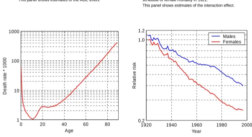
First, to capture the general pattern in mortality decline I fitted Model (1) to all ages. The female population in the year 1921 was selected as a reference group, which means that the AGE effect is close to the female death rates observed in that year. This estimated schedule of death rates, shown in Figure 1a, appears similar to those of other countries: a high peak of infant mortality, a bump of mortality in the 20s and then an exponential increase until the highest ages. The attentive reader will also have noticed “steps” of death rates at ages 40, 50, 60, 65, 70, and 80 – these are due to age heaping at these ages.
The interaction term of the fit (YEAR*SEX) is plotted in Figure 1b on the logarithmic scale. Every point on this graph can be interpreted as a ratio of the standard mortality schedule (Figure 1a) to a mortality schedule observed in a particular year and population. For example, the estimate for the male population in 1921 (first point on the blue curve) is 1.09, which means that male mortality in 1921 was on average 9% higher than female mortality in the same year. If we look at the last points reached by both curves in 1997, for females the estimate is 0.25 and for males 0.40. Thus, the level of female mortality in 1997 is about 25% and that of male mortality in 1997 is about 40% of the female mortality level in 1921.
As can be seen in Figure 1b, until the mid-1930s the excess of male mortality is rather small and the rate of decline is comparable to that of the female population. From this time onwards, female mortality started to decline faster than male mortality, the level of which nearly stagnated in the mid-1950s. Such differences in mortality trends led to the emergence of a gap between male and female death rates, which peaked in the mid-1970s. In later years the decline in female mortality slowed, however, while male death rates decreased at a higher rate. In most recent years the death rates for males and females are converging, thereby reducing the gap which had emerged before.
It would be an oversimplification to expect that Model (1) will fit the entire data set well, but it conveniently summarizes the sex differentials in mortality decline over time in one graph – much the same as it is summarized by life expectancy at birth. An analysis of goodness of fit,
which is not included here, shows that the model, indeed, does not fit the data very well3, but
nevertheless the results are included in the report because they are helpful for revealing the general trends.
The trends in individual age groups can be quite different from the average shown in Figure 1. To explore the dynamics of death rates more closely I fitted Model (1) separately for
3 To assess goodness of fit I computed deviance residuals and plotted them in the form of a Lexis map (not
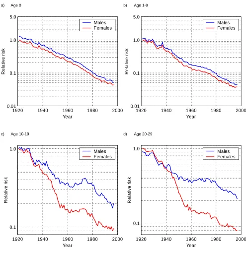
10-year age groups and plotted the interaction term in a similar fashion in Figure 2. The AGE effects are not shown in this figure since AGE has been used only as a control variable.
We can see that the most striking reductions in mortality occurred in infancy (age 0) and childhood (1–9 years of age), where death rates declined markedly and remarkably uniformly for both sexes, thus making the sex differential in mortality at these ages very small at the end of the 1990s. For females, the estimate in 1997 at age 0 is about 0.04 which means that the death rate at this age fell by a factor of 25 since 1920. In the most recent year death rates continued to decline at a similar rate as before, even though they had already reached exceptionally low levels until 1990.
Trends at young and young adult ages (10–19, 20–29, 30–39, and 40–49 years of age) show a pattern quite different from that found in other age groups. Until the mid-1950s death rates fell extremely rapidly both for males and females, but then they stagnated to a large extent and even increased for males at ages close to 20 in the 1970s and at ages 30-39 in the 1990s. Starting with the year 1980 the mortality decline for males and females accelerated again and death rates resumed their decline at a rate comparable with that before 1950. Another interesting feature of these graphs is that female mortality exceeded male mortality in the 1930s (Figures 2d and 2e). This excess of female mortality is not found on any of the other graphs. Males suffer from higher mortality throughout the whole period and age range analyzed.
At ages 50–59 and 60–69 female mortality declined more or less at a constant rate over the whole period of observation. This is indicated by almost linear downward trends in the female death rates (Figures 2g and 2h). In the male population at the same ages, trends in death rates have been quite different. Until 1970 virtually no changes in male mortality are to be observed. The death rates stayed at an almost constant level. It was only after 1970 that they started to decline. The rate of decline, however, was higher than the rate of decline observed in the female population during the period 1970-1997. This has led to a convergence of the levels of male and female death rates in the most recent years.
At older ages (Figure 2i and 2j) death rates decline more or less uniformly for both sexes. The level of mortality was almost the same for males and females in the 1920s, but due to the higher rate of mortality decline in the female population, the curves diverged over time. At the end of the 1970s mortality decline in the male population at ages 70-79 accelerated appreciably and the gap between the sexes was reduced in this age group.
this period4, mortality at each age has declined exponentially at a roughly constant rate" [Tuljapurkar et al. 2000]. If this would be the case the curves shown in Figure 2 would be well approximated by a linear function for the years 1950 onwards. However, it is clear that the pattern of mortality decline is much more complicated, especially for males. At ages 50-70, for example, it is clear that male death rates remained on a constant level until the late 1970s and only then started to decline. It seems to be the case that the Lee-Carter model summarizes information in matrix of death rates in some important ways but it doesn’t provide a good fit to the data.
4. Excess of male mortality over age and time
The analysis conducted in the previous section shows that the relative difference between male and female mortality was not constant, neither over age nor time. Hence, a simple proportional
hazard model5 of type:
YEAR + AGE + SEX (2)
will not be appropriate to capture the differences in survival between the sexes. I therefore decided to split the entire data set into ten-year age and calendar year periods and to fit Model (2) separately to each of the smaller data segments.
Table 1 shows the estimates of the SEX parameter. It shows the ratio of male to female mortality adjusted for age- and period-specific differences in mortality. Consider, for example, the period 1921–29 and age group 80–89. The SEX estimate is 1.05, which means that the male death rates were on the average 5% higher than those of females in this period at these ages. I have also fitted a nested model YEAR + AGE and compared it with (2) using the likelihood ratio to check whether the estimate of the SEX parameter is significant. It turns out that the estimate is not significant only for the age group 40–49 in the period 1921–29. In all other cases the p-values are less than 0.001.
As follows from Table 1, the smallest differences in survival between the sexes are observed in the period 1921–1940. Females even experienced higher mortality in the age group 20–50, as is indicated by the table cells with a blue background. Starting with the 1940s, male mortality was higher than female mortality at virtually all ages, and this difference increased over time, especially at young adult ages. Male mortality is now more than double female mortality at these ages.
4
1950-1994
5 The model specifies that death rate m
ijk is proportional to the current year, age, and sex mijk = yi aj sk,where yi is the
Table 1:
Estimation of the excess of male mortality controlled by year and age.
Ages Period
1921-29 1930-39 1940-49 1950-59 1960-69 1970-79 1980-89 1990-97 0 1.32 1.30 1.27 1.28 1.28 1.28 1.27 1.23 1-9 1.12 1.17 1.22 1.31 1.34 1.34 1.30 1.24 10-19 1.06 1.11 1.37 1.91 2.15 2.40 2.43 2.13 20-29 0.91 0.95 1.19 2.03 2.69 2.92 2.98 2.86 30-39 0.84 0.90 1.07 1.49 1.75 1.82 2.00 2.25 40-49 0.98* 1.07 1.25 1.49 1.72 1.81 1.68 1.70 50-59 1.11 1.17 1.35 1.69 1.91 2.00 1.89 1.70 60-69 1.11 1.18 1.34 1.58 1.86 2.05 2.01 1.86 70-79 1.10 1.13 1.21 1.33 1.55 1.79 1.88 1.81 80-89 1.05 1.09 1.11 1.18 1.26 1.43 1.56 1.57
estimates below 1 (female mortality is higher than male)
estimates which are greater than 1 but less than 2 (male mortality is moderately higher than female) estimates which are above 2 (male mortality is much higher than female)
* Not significant, p-value = 0.054 with 1 DF. All other estimates are significant at the 0.001 level.
Trends in sex differences over age and time can be presented more clearly by plotting the data from Table 1 by age groups and periods (Figure 3). Figure 3a shows estimates of the sex ratio plotted by age group. Almost constant curves for the age groups 0 and 1–9 reflect the fact that mortality decline occurred almost parallel for boys and girls. This is consistent with the findings in the previous section (Figures 2a and 2b): although the death rates fell dramatically in these age groups, the pattern of decline was similar for both sexes. The second important finding is that the difference in death rates by sex rose until the mid-1980s and then started to decline. This is indicated by the almost bell-shaped patterns of most of the curves. The only exceptions from this pattern are ages 30–39 and 80–89. For them the relative difference between males and females increased continuously over the entire period.
Figure 3b makes it easier to follow changes in the age pattern of mortality differences over time. We can see, for example, that there were dramatic changes in the pattern of the sex ratio at ages 10–40. During the period 1921–49 the death rates for males and females were fairly close but in the later years the sex ratio dramatically increased and reached a level of 2.5 and higher for the age group 20–29. This means that male death rates in this age group have been more than 2.5 times higher than for females over the last four decades.
5. Visualization of sex-specific differences in survival
There are a number of methods for visualizing demographic data [Vaupel et al. 1998] and in this section I am going to demonstrate how these methods can be applied to the analysis of Canadian mortality. Using death counts and exposure estimates we can compute death rates by single year and age, and then plot them as a Lexis map. In terms of intensity regression this is equivalent to fitting the YEAR*AGE model to each sex alone. Figure 4, for example, shows a Lexis map of
Canadian male death rates computed this way6. The scale on the right partitions all death rates
into groups and the death rates included in a given group are assigned the same color. For example, all death rates which are less than 0.0005 are plotted in dark blue as indicated by the lowest scale rectangle. Similarly, all death rates which are higher than 0.0005 and lower than 0.002 are plotted in ordinary blue (second rectangle on the scale from the bottom) and so on.
The contour maps of Canadian mortality presented in Figures 4 and 5 permit us to see all death rates at a glance. The contour lines themselves help us to follow the development of mortality over age and time. If we look at contour line 0.016 (Figure 4), for example, which separates light blue from light magenta, we can see that it remains almost constant at age 58 up to the year 1980 and only after this year does it start to rise. This indicates that mortality in this age group did not undergo any significant changes until 1980 and only then began to decline. This observation confirms findings in death rates shown in Figure 2 for ages 50-80. For females, however, mortality developments at adult ages have been quite different. Contour lines have been steadily rising for virtually all ages over the whole period of observation. This is an indication of persistent progress made against mortality, a pattern very different from what we observe in the male data.
The dark blue area in Figures 4 and 5 shows the lowest levels of death rates ever reached in the Canadian population. We can see that, for females, this area started to emerge in the 1950s and over time it spread out to cover more ages. For males the region of lowest mortality is less pronounced, and it did not become evident until the mid-1960s. It, too, has spread out over time but in contrast to females only to young ages. Additionally, a light blue area in the year 1975 at age 20 shows the ages and years where mortality in the male population in fact increased (it is also visible, though less distinctly, in Figures 2c and 2d). Finally, to provide the reader with an overview of the amount of the information presented, let us state that Figures 4 and 5 include information on 13,860 death rates, displaying them in a concise and revealing manner.
In order to reveal age-specific differences in Canadian survival I divided the matrix of male death rates by the matrix of female death rates and then plotted the result as a Lexis map (Figure 6). In this map the elements that exceed 1 in the sex ratio matrix are colored in magenta hues and the elements less than 1 in blue. Thus, magenta shows the area with higher male
6 This figure has been produced with the help of the program Lexis. This program is a part of Ph.D. thesis2 and can
mortality and blue with lower. We can see, for example, that females had a mortality excess at ages 20–50 in the years 1921–1940. This area of excessive female mortality completely disappeared before 1940, at which point the gap between male and female mortality started to emerge. It is apparent from Figure 6 that the gap started to form in two distinct age groups. The first group consists of the young ages: already in the 1950s male death rates at age 20 were twice as high as female death rates. Over time the difference only became aggravated and spread to cover older ages as well. Now male death rates at ages 17–35 are from 2 to 2.5 times higher than the corresponding female death rates.
Another age group which suffered from exceptionally high excess male mortality covers the senior ages (55–70). The difference in death rates shows quite a different pattern, however. It started to rise in the 1940s, reached a peak in 1980, and declined afterwards. The area of male death rates, which were more than twice as high as for females, appears on the map as a distinct, eye-catching ellipse which virtually disappears in the 1990s. In most recent years the difference between male and female death rates has continued to decline at these ages.
The World Health Report 1999 [WHO 1999] reports Canadian life expectancy at birth to be 71 for males and 78 for females in the year 1978 and 76 and 82 in 1998, respectively. As we just learned in this section, the convergence in life expectancy between the sexes is now driven mostly by the behavior of death rates at senior ages. This overall convergence is occurring despite the fact that at young ages the sex differences are increasing over time. The level of mortality at young ages is very low now and this diverging trend cannot affect the trends in life expectancy in any important way.
Finally, returning to Model (2) I would like to note that Figure 6 provides further evidence of the fact that a simple proportional model will not fit the whole data set appropriately. Such a model will try to catch the male–female difference by means of a single parameter, but the pattern is much more complicated.
6. Conclusions
The present report demonstrates how intensity regression techniques can be applied to study age-and period-specific differences in survival between males age-and females in Canada. In the previous section I have also shown how the same phenomenon can be studied with the help of visualization techniques. A brief illustration of the character of the results obtained by both methods is presented as well.
• The data set includes only three covariates and it can be easily separated into male and female mortality maps.
• The data represent the entire population of Canada. This makes it possible to compute
reliable, direct estimates of the death rates, so the plots will not be disturbed by a high degree of stochastic noise.
If one or another of these conditions is not fulfilled the application of the visualization methods will be less appealing.
The intensity regression techniques allow us to conduct a more detailed analysis and to test the statistical significance of the estimates. Some important details can be revealed by intensity regression, which would be virtually invisible on the Lexis maps. For example, it is evident from Figures 2a and 2b that infant and childhood mortality increased significantly in 1937, but on the Lexis maps (Figures 4 and 5) this fact hardly attracts attention. In sum, intensity regression is a means of summarizing information in the data set in a concise, numeric manner whereas the Lexis maps provide a visualization of the entire data array.
The analysis conducted here shows that the choice of analytical method should be driven not only by the information present in the data set (occurrences and exposures) but by the structure of the data as well. If the structure is very simple, as was the case for what we have analyzed here, the visualization techniques might prove to be as useful as regression techniques.
Also I would like to note that the age-specific differences in Canadian survival (Fig. 6) are strikingly similar between those found for other countries [Andreev 1999]. There are still some differences between the Lexis maps but there are far more similarities to be observed. It might be the case that there exist certain factors like smoking prevalence that affect mortality in some uniform way, thereby maintaining a more or less fixed pattern of male-female differences over various countries.
Excess of male mortality over the last decades is a well-known phenomenon and a number of hypotheses have been put forward as possible explanations [Nault 1997, Waldron 1983; Waldron 1993]. These hypotheses are based mainly on analysis of cause-specific mortality, social and behavioral differences, risk factors prevailing in male and female populations, and inherent biological and genetics differences. Complete analysis of observed differences in survival between sexes in Canada is well beyond the scope of this paper, so I limit myself to a brief overview of possible explanations.
after that period started to decline7. For females, however, the death rates declined almost in linear fashion over the years 1950-97: the death rates fell from the level 800 deaths per 100,000 at the beginning of 1950s to 200 in the middle of 1990s. As a result, the sex ratio of mortality from this cause of death significantly increased over 1950-80, then stagnated at a level about 2.7, and finally dropped slightly in the 1990s.
On the other hand, trends in cancer mortality were very different from those observed for CVDs. For females, the level of mortality was more or less constant over the years 1950-97 while male death rates were increasing up to the year 1990 and then sharply declining, thereby reducing the gap between male and female mortality. The relative difference between sexes is less pronounced compared to CVDs. Over the 1980s male death rates were only 1.5 times higher than females. This analysis of cancer mortality indicates that a change in this cause of death is the main driving force behind the convergence of male and female death rates during the 1990s. Especially unfavorable trends are to be observed in the female death rates due to lung cancer. The death rates have been persistently increasing since the late 1960s while male death rates have been declining since the late 1980s. As a result, the huge excess of male mortality (over the years 1950-70 male death rates were about 8 times higher than female at ages 55-75) has been significantly reduced and now male death rates are approximately only two times higher than female death rates now.
At young and young adult ages (15-35) the excess of male mortality during recent decades is mostly due to accidental causes. Death rates from suicide and traffic accidents were considerably higher for males than for females. On the contrary, prior to the 1950s female death rates were in fact higher than male, which is probably mostly attributable to maternal mortality and complications in childbearing. Improvements in health care system significantly reduced this component of female mortality. At the beginning of the 1950s an excess of female mortality completely disappeared.
We can see that analysis of trends in cause-specific mortality can highlight certain differences in survival between males and females but unfortunately it cannot provide a complete explanation of the observed differences in survival. More analysis will require investigation of risk factors prevailing in the male and female populations and their relation to mortality. Most researchers agree that smoking provides one of the main contributions to the observed mortality differences between both sexes and countries. However, the relation of this risk factor to trends in death rates is less clear. In Canada, for example, smoking rates have declined over the period 1977-95 for both males and females, but the level has always been higher for males than for females [Millar 1996]. Trends in lung cancer mortality, however, were quite different. For males they rose until the late 1980s and then started to decline for virtually all ages from 50 to 75. For females, however, the rates have been increasing persistently since 1970. It could be that
smoking affects females more than males so the relation between this risk factor and trends in lung cancer is not straightforward.
On the other hand, females have always had lower mortality from CVDs and trends in this cause of death were similar to those observed in the male population. This contradicts the fact that smoking is also a risk factor for CVDs. Lower female rates from CVDs can be partially explained by the protective effect of female sex hormones and better utilization of the health care system, genetic and social factors, respectively [Waldron 1983, Waldron 1993]. This demonstrates that the observed sex differences in survival are affected by a variety of causal factors. Their influence on mortality still calls for explanation.
7. Acknowledgements
This report is based mainly on material from the final mini-project completed by the author for the course “An Introduction to Regression Analysis of Duration Data (Event-History Regression)”, which was given by Prof. Jan M. Hoem during the winter semester 2000 at the Max Planck Institute for Demographic Research, Germany. I am grateful to Prof. Jan M. Hoem for supporting my work on this project and for making available free of charge the computer program Rocanova, written by Sten Martinelle of Statistics Sweden for estimation intensity regression models. Without this required mini-project this analysis would, no doubt, never have been conducted.
References
Andreev, K. F. Demographic surfaces: Estimation, Assessment and Presentation, with Application to Danish Mortality, 1835–1995. Ph.D. thesis: University of Southern Denmark, Odense, Denmark; 1999.
Hoem, Jan M. Statistical Analysis of a Multiplicative Model and its Application to the Standardization of Vital Rates: A Review. International Statistical Review. 1987; 55(2):119-152.
Hoem, Jan M. Harmless omission in the Standardization of Demographic Rates. European Journal of Population. 1995; 11:313-312.
Kleinbaum, David G., Kupper, Lawrence L., Muller, Keith E., and Nizam, Azhar. Applied Regression Analysis and Other Multivariable Methods. third ed. New York: Duxbury Press; 1998.
Lee, Ronald D. and Carter, Lawrence R. Modelling and Forecasting U.S. Mortality. Journal of the American Statistical Association. 1992 Sep; 87(419):659-675.
Millar, W. J. Reaching smokers with lower educational attainment. Health Reports, Statistics Canada. 1996; 8(2):11-9.
Nault, Francois. Narrowing mortality gaps, 1978 to 1995. Health Reports, Statistics Canada. 1997; 9(1):35-41.
Tuljapurkar, Shripad; Li, Nan, and Boe, Carl. A universal pattern of mortality decline in the G7 countries. Nature. 2000 Jun 15; 405.
Vaupel, J. W.; Zhenglian, W.; Andreev, K. F., and Yashin, A. I. Population Data at Glance: Shaded Contour Maps of Demographic Surfaces over Age and Time. Odense University, Denmark: Odense University Press; 1998; ISBN: 87-7838-338-2. Available online at http://www.demogr.mpg.de/Papers/PapersPres.htm.
Waldron, Ingrid. Sex differences in human mortality: The role of genetic factors. Social Science and Medicine. 1983; 17(6):321-333.
Waldron, Ingrid. Recent trends in sex mortality ratios for adults in developed countries. Social Science and Medicine. 1993; 36(4):451-462.
Figure 1:
Fit of Model (1) to Canadian death rates for the period 1921-1997 and ages 0-89.
a) Age-specific schedule of female mortality in 1921. This panel shows estimates of the AGE effect.
b) Trends in Canadian death rates relative to the age-specific schedule of female mortality in 1921.
This panel shows estimates of the interaction effect.
1920 1940 1960 1980 2000
0.2 1.0 1.2
R
e
la
ti
ve
r
isk
Year
Males Females
0 20 40 60 80
1 10 100 1000
D
eat
h r
a
te
*
1000
Figure 2:
Trends in Canadian death rates relative to the age-specific schedule of female mortality in 1921, separately for each selected age group.
These panels show estimates of the YEAR*SEX interaction term in Model 1. The AGE variable is only a control, so the age effects are not shown.
a) Age 0 b) Age 1-9
c) Age 10-19 d) Age 20-29
1920 1940 1960 1980 2000
0.01 0.1 1.0 5.0 R e la ti ve r isk Year Males Females
1920 1940 1960 1980 2000
0.01 0.1 1.0 5.0 R e la ti ve r isk Year Males Females
1920 1940 1960 1980 2000
0.1 1.0 R e la ti ve r isk Year Males Females
1920 1940 1960 1980 2000
e) Age 30-39 f) Age 40-49
g) Age 50-59 h) Age 60-69
1920 1940 1960 1980 2000
0.1 1.0
R
e
la
ti
ve
r
isk
Year
Males Females
1920 1940 1960 1980 2000
0.2 1.0
R
e
la
ti
ve
r
isk
Year
Males Females
1920 1940 1960 1980 2000
0.3 1.0
R
e
la
ti
ve
r
isk
Year Males
Females
1920 1940 1960 1980 2000
0.3 1.0
R
e
la
ti
ve
r
isk
Year Males
i) Age 70-79 j) Age 80-89
1920 1940 1960 1980 2000
0.3 1.0 1.3
R
e
la
ti
ve
r
isk
Year Males
Females
1920 1940 1960 1980 2000
0.4 1.0 1.3
R
e
la
ti
ve
r
isk
Year Males
Figure 3:
Sex ratio adjusted for age and year.
These figures are based on data from Table 1. Note that all groups are plotted equidistantly.
a) by age group b) by period
Figure 4: 0 0.5 1 1.5 2 2.5 3 3.5 0 1-9 10 -1 9 20 -2 9 30 -3 9 40 -4 9 50 -5 9 60 -6 9 70 -7 9 80 -8 9 Age group Se x r a ti o
1921-29 1930-39 1940-49 1950-59 1960-69 1970-79 1980-89 1990-97
0.0005 0.0020 0.0040 0.0080 0.0160 0.0640 0.2560
1921 1930 1940 1950 1960 1970 1980 1990 1998
0 10 20 30 40 50 60 70 80
90 Canada, Males
Death rates Year Age 0 0.5 1 1.5 2 2.5 3 3.5 1921-29 1930-39 1940-49 1950-59 1960-69 1970-79 1980-89 1990-97 Period Se x r a ti o
0 1-9 10-19 20-29 30-39
Figure 5:
Figure 6:
0.0005 0.0020 0.0040 0.0080 0.0160 0.0640 0.2560
1921 1930 1940 1950 1960 1970 1980 1990 1998
0 10 20 30 40 50 60 70 80
90 Canada, Females
Death rates
Year Age
0.80 1.00 1.20 1.50 1.80 2.00
1921 1930 1940 1950 1960 1970 1980 1990 1998
0 10 20 30 40 50 60 70 80
90 Sex ratio of Canadian mortality