On second derivative 3-stage Hermite--Birkhoff--Obrechkoff methods for stiff ODEs: A-stable up to order 10 with variable stepsize

(1)

On second derivative 3-stage Hermite–Birkhoﬀ–Obrechkoﬀ methods

for stiﬀ ODEs: A-stable up to order 10 with variable stepsize

Truong Nguyen-Ba∗

Department of Mathematics and Statistics,

University of Ottawa, Ottawa, Ontario, Canada K1N 6N5. E-mail: [email protected]

Thierry Giordano

R´emi Vaillancourt

Abstract Variable-step (VS) second derivative k-step 3-stage Hermite–Birkhoff–Obrechkoff (HBO) methods of orderp= (k+ 3), denoted by HBO(p) are constructed as a com-bination of lineark-step methods of order (p−2) and a second derivative two-step diagonally implicit 3-stage Hermite–Birkhoff method of order 5 (DIHB5) for solving stiff ordinary differential equations. The main reason for considering this class of for-mulae is to obtain a set ofk-step methods which areL-stable and are suitable for the integration of stiff differential systems whose Jacobians have some large eigenvalues lying close to the imaginary axis with negative real part. The approach, described in the present paper, allows us to developL-stablek-step methods of order up to 10. Selected HBO(p) of order p,p= 9,10, compare favorably with existing Cash

L-stable second derivative extended backward diﬀerentiation formulae, SDEBDF(p),

p= 7,8 in solving problems often used to test stiﬀ ODE solvers.

Keywords. Hermite–Birkhoff methods, generalized DIRK methods, A-stable, oscillatory stiff DETEST problems, confluent Vandermonde-type systems.

2010 Mathematics Subject Classification. 65L06, 65D05, 65D30.

1. Introduction

For solving stiﬀ ordinary diﬀerential equations (ODE),

y′ =f(t, y), y(t0) =y0, where ′= d

dt and y∈R

n_, _(1.1)

a linear k-step method of order p−2 and a second derivative two-step diagonally implicit 3-stage Hermite–Birkhoff method of order 5 (DIHB5) are cast into ak-step 3-stage Hermite–Birkhoff–Obrechkoff (HBO) methods of orderp= (k+ 3), denoted

Received: 26 March 2017 ; Accepted: 24 September 2017.

∗Corresponding author.

(2)

by HBO(p). The method’s name was chosen because it uses Hermite–Birkhoff inter-polation polynomials, first and second order derivatives ofy like Obrechkoff methods [20]. Here, the DIHB5 is defined in Section2withp= 5 and step numberk= 2, and has three degree of freedom since the coefficients in (2.4) are free parameters. And, following the approach of Cash [3], the abscissae ci are allowed to be 0 ≤ ci ≤ 2, i= 2,3,4.

There is a variety of variable step (VS) methods designed to solve nonstiff and stiff systems of first-order differential equations (ODEs). Gear advocated a quasi-constant step size implementation in DIFSUB [9]. This software works with a constant step size until a change of step size is necessary or clearly advantageous. Then a continuous extension is used to get approximations to the solution at previous points in an equally spaced mesh. This was largely because constant mesh spacing is very helpful when solving stiff problems. Another possibility is fixed leading coefficient, which is seen in Petzold’s popular code DASSL [21]. Finally, the actual mesh can be chosen by the code as done in MATLAB’sode113. This is the equivalent of a PECE Adams formula in contrast with the Adams–Moulton formula of DIFSUB and DASSL. In this paper, a fully variable step size implementation is used with actual mesh.

A more basic point about the implementation of a method is the choice of the form. The present method uses a generalized Lagrange form and much of the paper is devoted to computing the coefficients efficiently. Remark 6.1 in Subsection 6.2 connects the computation of coefficients for three well known forms: generalized La-grange form, generalized Newton divided differences form (similar to Krogh’s modified divided differences [16]) and Nordsieck form [19].

A brief survey of methods for the numerical integration of (1.1) reveals that there are many advances in the class of generalized linear multistep methods for stiff ODEs, methods like second derivative multistep methods (SDMM) proposed by Enright [5], second derivative extended backward differentiation formulas (SDEBDF) by Cash [3], second derivative BDF methods (SDBDF) by Haireret al. [10], special classes of SDMM introduced by Ismailet al. [14], Hojjatiet al. [12] and Khalsaraeiet al. [15]. The first modification, introduced by Cash [3], was the SDEBDF in which one “super-future” point has been applied.

The current investigation and the results are offered as potentially useful additions to the contemporary repertory of variable step (VS)L-stable second derivative multi-step solvers for stiff differential equations (ODEs). This paper explores an alternative way to improve the order ofL-stable second derivative multistep methods.

(3)

The extra stability is particularly important when integrating stiff differential sys-tems whose Jacobians have some large eigenvalues lying close to the imaginary axis. Stiff oscillatory problems happen often in practice. In particular, they frequently de-velop when the method of lines technique is applied to a system of partial differential equations (PDE) that have some hyperbolic type of behaviour. Typical examples of such problems are the integro-differential equations describing the stiff beam problem [10], and advection-dominated PDE problems, as described, for example, in [11,23]. A good description of the difficulties involved in integrating these hyperbolic type equations can be found in [10, pp. 12].

The selected HBO(p),p= 9,10 compare favorably with SDEBDF(p),p= 7,8, [3] in solving problems often used to test highly stable stiﬀ ODE solvers on the basis of number of steps (NS), CPU time (CPU) and the error at the endpoint (EPE) of the interval of integration.

The paper is organized as follows: in Section 2, we introduce new general VS HBO(p) methods of order p. Order conditions of general VS HBO(p) are listed in Section3. In Section4, particular variable step HBO(p) are defined by fixing a set of parameters and are represented in terms of Vandermonde-type systems. In Section5, symbolic elementary matrices are constructed as functions of the parameters of the methods in view of factoring the coefficient matrices of Vandermonde-type systems. Fast solution of Vandermonde-type systems for variable step HBO(p) is constructed in Section 6. Section 7 considers the regions of absolute stability of constant step L-stable HBO(p),p= 5,6, . . . ,10. Section8deals with the step control. In Section9, we compare the numerical performance ofL-stable methods considered in this paper. AppendixA lists the algorithms. Appendix Blists the coefficients of constant step L-stable HBO(p) methods of orderp= 9,10.

2. _{General variable step HBO}(p)_{of order} p

Variable step 3-stage HBO methods are constructed by the following formulae to perform integration fromtn totn+1.

Lethn+1 denote the step size. The abscissa vector [c1, c2, c3, c4]T deﬁnes the oﬀ-step pointstn+cjhn+1 withc1= 0 andc4= 1. Following the approach of Cash [3], ci are allowed to be 0≤ci≤2,i= 2,3.

Let F1 = fn and Fj := f(tn +cjhn+1, Yj), j = 2,3,4, denote the jth stage derivative.

With the initial stage value,Y1=yn, HB polynomials are used as implicit predic-tors Pi to obtain the stage valuesYi to orderp−2,

Yi=hn+1aiif(tn+cihn+1, Yi) +h2n+1γiif′(tn+cihn+1, Yi)

+yn+hn+1

[p_∑−4

j=0

βijfn−j+ i−1

∑

j=2 aijFj

]

+h2_n+1 i−1

∑

j=2

(4)

An HB polynomial is used as implicit integration formula IF to obtain yn+1 to orderp,

yn+1=hn+1b4f(tn+hn+1, yn+1) +h2n+1g4f′(tn+hn+1, yn+1)

+yn+hn+1

[p_∑₋4

j=0

βjfn−j+ 3

∑

j=2 bjFj

]

+h2n+1g3F3′. (2.2)

An HB polynomial is used as implicit predictor P4 to control the step size,hn+2, and obtainyen+1 to orderp−2,

e

yn+1=hn+1a44f(tn+hn+1, yn+1) +h2n+1γ44f′(tn+hn+1, yn+1)

+yn+hn+1

[p_∑₋4

j=0

β4jfn−j+ 3

∑

j=2 a4jFj

]

+h2_n+1γ43F3′. (2.3)

Here, the forms (2.1) and (2.2) are used by the implicit algebraic equations system deﬁningYi,i= 2,3 andyn+1 to handle implicitness in the context of stiﬀness.

The distinct implicit algebraic equations systems (2.1) and (2.2) deﬁningYi,i= 2,3 andyn+1 are solved iteratively by the modiﬁed Newton–Raphson method similar to the usual resolution of system of implicit algebraic equations of BDF method [17, p. 11–13].

The following terminology will be useful. An HBO(p) method is said to be ageneral variable-step HBO method if its backstep and the coeﬃcients

c2, c3, a22=a33=b4, (2.4)

in (2.1) and (2.2) are variable parameters. Hence, the general variable-step HBO method has three degrees of freedom (c2, c3, a22 =a33 = b4). If the coefficients in (2.4) are fixed, the method is said to be a particular variable-step method. If the step size is constant, and hence the backsteps and the coefficients in (2.4) are fixed parameters, the method is said to be aconstant-step method.

3. _{Order conditions of general HBO}(p)

To derive the order conditions of 3-stage (p−3)-step HBO(p), we shall use the following expressions coming from the backsteps of the methods:

Bi(j) = p₋4

∑

ℓ=1 βiℓ

η_ℓ+1j−1

(j−1)!,

{

i= 2,3,

j= 1,2, . . . , p, (3.1)

and

ηj=− 1 hn+1

(tn−tn+1₋j) =− 1 hn+1

j−2

∑

i=0

hn₋i, j= 2,3, . . . , p−3. (3.2)

In the sequel,ηj will be frequently used without explicit reference to (3.2).

(5)

multistep-and several Runge–Kutta(RK)-type order conditions that must be satisﬁed by 3-stage HBO(p) methods.

To reduce a large number of RK-type order conditions (see [18]), we impose the following simplifying assumptions:

i

∑

j=2 γij

ck_j−1

(k−1)! + i

∑

j=2 aij

ck_j

k! +Bi(k+ 1) = ck+1_i (k+ 1)!,

{

i= 2,3,

k= 0,1, . . . , p−3.

(3.3)

Thus, there remain only two sets of equations to be solved:

4

∑

i=3 gi

ck_i−1 (k−1)! +

4

∑

i=2 bi

ck i

k! +B(k+ 1) = 1

(k+ 1)!, k= 0,1, . . . , p−1, (3.4)

4

∑

i=3 gi

cp_i−2 (p−2)!+

3

∑

i=2 bi

[∑i

j=2 γij

cp_j−3

(p−3)! + i

∑

j=2 aij

cp_j−2

(p−2)! +Bi(p−1)

]

+b4 cp₄−1

(p−1)!+B(p) = 1

p!, (3.5)

where the backstep parts,B(j), are deﬁned by

B(j) = p−4

∑

ℓ=1 βℓ

ηj_ℓ+1−1

(j−1)!, j= 1,2, . . . , p+ 1. (3.6)

These order conditions are simply RK order conditions with backstep partsBi(·) and B(·).

4. _{Vandermonde-type formulation of particular variable step HBO}(p)

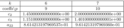
The general HBO(p) methods obtained in Section3contain free coeﬃcients in (2.4), and depend onhn+1 and the previous nodes,tn, tn−1, . . . , tn−(p−4), which determine η2, η3, . . . , ηp−3 in (3.2). To obtain A-stability of particular HBO(p) methods, p = 9,10, the coeﬃcients listed in Table1 were chosen. In Table1, sincea22=a33=b4, only values ofa22are listed.

It is to be noted that, to obtain the coeﬃcients in Table1, the well-known exhaus-tive search method is used with possible candidates (c2, c3, a22), for c2 = 0.1,0.15, 0.2, . . . ,2.0, c3 = 0.1,0.15, 0.2, . . . ,2.0 and a22 with the same increment (or decre-ment) size 0.05. The value ofa22 which yields the largestαofA(α)-stability is used as a starting value (the exhaustive search method can be repeated with new starting values ofa22).

(6)

Table 1. Coeﬃcientsci,i= 2,3 anda22 (=a33=b4) of particular VS HBO(p),p= 9,10.

k 6 7

coeﬀs\p 9 10

c2 1.450000000000000e+00 2.000000000000000e+00

c3 1.151000000000000e+00 1.401000000000001e+00

a22 8.614213197969537e-01 9.614213197969360e-01

4.1. Predictor P2. The (p−2)-vector of reordered coeﬃcients of the predictor P2 in (2.1) withi= 2,

u2= [β20, β21, . . . , β2,p−4, γ22]T,

is the solution of the Vandermonde-type system of order conditions

M2u2=r2, (4.1)

where

M2=

            

1 1 1 · · · 1 0

0 η2 η3 · · · ηp−3 1

0 η22

2!

η2 3

2! · · ·

η2_p₋₃

2! c2

0 η

3 2

3!

η3₃

3! · · ·

η3 p−3

3!

c2₂

2! . . . . . . 0 η

p−3 2

(p−3)!

η₃p−3

(p−3)! · · ·

η_pp−₋3₃

(p−3)!

cp₂−4

(p−4)!              , (4.2)

andr2₌_r

2(1 :p−2) has components

r2(i) = c i 2 i! −a22

ci₂−1

(i−1)!, i= 1,2, . . . , p−2.

A truncated Taylor expansion of the right-hand side of (2.1) with i= 2 about tn gives

p+1

∑

j=0 S2(j)h

j n+1y

(j) n

with coeﬃcients

S2(j) =a22 cj₂−1 (j−1)! +M

2₍_j,_{1 :}_p₋₂₎_u2

=a22 cj₂−1

(j−1)! +r2(j) = cj₂

j!, j= 1,2, . . . , p−2,

S2(j) =a22S2(j−1) + p₋4

∑

i=1 β2i

η_i+1j−1

(j−1)!, j=p−1, p, p+ 1.

We note that P2 is of orderp−2 since it satisﬁes the order conditions

S2(j) =c j

(7)

and its leading error term is

[

S2(p−1)− cp₂−1 (p−1)!

]

hp_n+1−1y_n(p−1).

4.2. Integration formula IF. Thep-vector of reordered coeﬃcients of the integra-tion formula IF in (2.2),

u1= [β0, b3, b2, β1, β2, . . . , βp−4, g3]T,

M1u1=r1, (4.3)

where

M1=

         

1 1 1 1 1 · · · 1 0

0 c3 c2 η2 η3 · · · ηp−3 1

0 c23

2! c2 2 2! η2 2 2! η2 3

2! · · ·

η2_p₋₃

2! c3 . . . . . . 0 c

p−1 3

(p−1)!

cp₂−1

(p−1)!

η₂p−1

(p−1)!

ηp₃−1

(p−1)! · · ·

ηp_p₋−₃1

(p−1)!

cp₃−2

(p−2)!           , (4.4)

andr1₌_r_{1(1 :}_p_{) has components}

r1(1) = 1−b4,

r1(i) = 1 i!−b4

ci₄−1 (i−1)! −g4

ci₄−2

(i−2)!, i= 2,3, . . . , p,

whereb4=a22andg4=γ22. The leading error term of IF is

[

g4 cp₄−1 (p−1)! +b4

cp₄ p! +

p−4

∑

j=1 βj

η_j+1p

p! + 3

∑

j=2 bj

cp_j

p! +g3 cp₃−1 (p−1)!−

1 (p+ 1)!

]

hp+1_n+1y_np+1.

4.3. Predictor P3. We consider the (p−1)-vector of reordered coeﬃcients of the predictor P3in (2.1) withi= 3,

u3= [β30, a32, β31, . . . , β3,p−4, γ32]T,

M3u3=r3, (4.5)

where

M3=

       

1 1 1 1 · · · 1 0

0 c2 η2 η3 · · · ηp−3 1

0 c22 2! η2 2 2! η2 3 2! · · ·

η2 p−3

2! c2

..

. ...

0 c

p−2 2 (p−2)!

ηp₂−2 (p−2)!

ηp₃−2 (p−2)! · · ·

η_pp−₋2₃ (p−2)!

cp₂−3 (p−3)!

(8)

The ﬁrst (p−2) components ofr3=r3(1 :p−1) are

r3(1) =c3−a33,

r3(i) = ci

3 i! −a33

ci₃−1

(i−1)!−γ33 ci₃−2

(i−2)!, i= 2,3, . . . , p−2,

the (p−1)th component is

r3(p−1) =S3(p−1)−a33 cp₃−2

(p−2)!−γ33 cp₃−3

(p−3)!, (4.7)

where

S3(p−1) = 1 b3

[

1

p!−b2S2(p−1)−b4 cp₄−1 (p−1)!

−g3 cp₃−2 (p−2)! −g4

cp₄−2

(p−2)! −B(p)

]

,

a33=a22 andγ33=γ22.

The equation forr3(p−1) in (4.7) corresponds to order condition (3.5).

A truncated Taylor expansion of the right-hand side of (2.1), withi= 3, abouttn gives

p+1

∑

j=0

S3(j)hj_n+1y(j)_n

with coeﬃcients

S3(j) =a33 cj₃−1

(j−1)! +γ33 cj₃−2 (j−2)! +M

3₍_j_{+ 1}_,_{1 :}_p₋₁₎_u3

=a33 cj₃−1

(j−1)! +γ33 cj₃−2

(j−2)! +r3(j) = cj₃

j!, j= 1,2, . . . , p−2, S3(j) =a33S3(j−1) +γ33S3(j−2) +a32S2(j−1) +γ32S2(j−2)

+ p−4

∑

i=1 β3i

η_i+1j−1

(j−1)!, j =p−1, p, p+ 1.

4.4. Step control predictor P4. The (p−2)-vector of reordered coeﬃcients of predictor P4in (2.3),

u4= [β40, a42, β41, . . . , β4,p−4]T,

is the solution of the system of order conditions

(9)

where

M4=

         

1 1 1 1 · · · 1

0 c2 η2 η3 · · · ηp−3

0 c22

2!

η2₂

2!

η₃2

2! · · ·

η2_p₋₃

2!

. . .

0 c

p−3 2

(p−3)!

η₂p−3

(p−3)!

η₃p−3

(p−3)! · · ·

ηp_p−₋3₃

(p−3)!          

, (4.9)

andr4₌_r

4(1 :p−2) has components

r4(1) = 1−(b4+ω4)−(b3+ω3),

r4(i) = 1

i!−(g4+ω

′

4) ci₄−2

(i−2)! −(b4+ω4) ci₄−1 (i−1)!

−(g3+ω′3) ci₃−2

(i−2)! −(b3+ω3) ci₃−1

(i−1)!, i= 2,3, . . . , p−2.

For arbitrary nonzeroω3and ω3′, P4 yieldsyen+1 to order (p−2). A good experi-mental choice isω3= 0.025,ω′3= 0.025,ω4= 0.025,ω4′ = 0.025.

The solutionsuℓ_, _ℓ_{= 1}_,₂_,₃_,_{4, form generalized Lagrange basis functions for} rep-resenting the HB interpolation polynomials.

5. _{Symbolic construction of elementary matrix functions}

Consider the matrices

Mℓ∈Rmℓ×mℓ_, _ℓ_{= 2}_,₁_,₃_,₄_, _(5.1)

of the Vandermonde-type systems (4.1), (4.3), (4.5) and (4.8), where

m2=p−2, m1=p, m3=p−1, m4=p−2, (5.2)

andpis the order of the method.

The purpose of this section is to construct elementary lower and upper triangular matrices as symbolic functions of the parameters of HBO(p). These matrices are most easily constructed by means of a symbolic software. These functions will be used in Section6to factor

• Mℓ _{into a diagonal+last-1-column matrix,} _Wℓ

1, ℓ = 2,1,3, which will be further diagonalized by a Gaussian elimination,

• M4_{into the identity matrix}_I4_.

This decomposition will lead to a fast solution of the systemsMℓ_uℓ₌_rℓ_,_ℓ_{= 2}_,₁_,₃_,₄ in O(p2_{) operations.}

(10)

5.1. Symbolic construction of lower bidiagonal matrices forMℓ,ℓ= 1,2,3,4. We ﬁrst describe the zeroing process of a general vectorx= [x1, x2, . . . , xm]T with no zero elements. The lower bidiagonal matrix

Lk=        

Ik−1 0 0 · · · 0

0 1 0 0

0 −τk+1 1 0

. . .

. .

. . .. . .. ...

0 0 0 −τm 1

       

, (5.3)

deﬁned by the multipliersτi = _xxi

i−1 =−Lk(i, i−1), i=k+ 1, k+ 2, . . . , m, zeros the last (m−k) components, xk+1, xk+2, . . . , xm, of x. This zeroing process will be applied recursively onMℓ,ℓ= 1,2,3,4, as follows. Fork= 2,3, . . ., left multiplying T_kℓ = Lℓ_k₋₁Lℓ_k₋₂· · ·L3ℓLℓ2Mℓ by Lkℓ zeros the last (mℓ −k) components of the kth column ofTℓ

k. Thus we obtain the upper triangular matrix

LℓMℓ=Lℓ_m

ℓ−1· · ·L ℓ 3L

ℓ 2M

ℓ_, _ℓ_{= 1}_,₂_,₃_,₄_, _(5.4)

in (mℓ−2) steps, forℓ= 1,2,3,4.

We note thatLℓ _{does not change the ﬁrst two rows of}_Mℓ_.

Process 1. At thekth step, starting withk= 2,

• Mℓ(k−1)₌_Lℓ k−1L

ℓ k−2· · ·L

ℓ

2Mℓis an upper triangular matrix in columns 1 to k−1,

• The multipliers inLℓ

kare obtained fromM

ℓ(k−1)₍_k_{+1 :}_m

ℓ, k) sinceMℓ(i, k)̸= 0 fori=k+ 1, k+ 2, . . . , mℓ.

Algorithm1in AppendixAdescribes this process. The input isM =Mℓ_;_m₌_m_ℓ. The output isLk=Lℓk,k= 2,3, . . . , mℓ−1,ℓ= 1,2,3,4.

5.2. Symbolic construction of upper bidiagonal matrices forMℓ,ℓ= 1,2,3,4. For matrix LℓMℓ, ℓ = 1,2,3,4, we construct recursively upper bidiagonal matrices U1ℓ, U2ℓ. . . , Ukℓℓ

end

such that right multiplying LℓMℓ by the upper triangular matrix

Uℓ ₌ _Uℓ

1U2ℓ· · ·Ukℓℓ end

transforms Lℓ_Mℓ _{into a matrix} _Wℓ

Cℓ = L

ℓ_Mℓ_Uℓ _{with nonzero}

diagonal elements,W_Cℓ

ℓ(i, i)̸= 0,i= 1,2, . . . , mℓ, the lastCℓnonzero columnsW ℓ

Cℓ(1 :

mℓ, j)̸= 0,j=mℓ− Cℓ+ 1, mℓ− Cℓ+ 2, . . . , mℓ, and zero elsewhere. We call such a matrix a “diagonal+last-Cℓ-column matrix”. Here

C1= 1, C2= 1, C3= 1, C4= 0, (5.5)

k_end1 =m1−2, kend2 =m2−2, k3end=m3−2, k4end=m4−1, (5.6)

forMℓ_, _ℓ_{= 1}_,₂_,₃_,_{4, respectively.}

We describe the zeroing process of the upper bidiagonal matrixUℓ

(11)

(LℓMℓ)(k:k+ 1,1 :mℓ)U1ℓU

ℓ

2· · ·U

ℓ k−1

=

[

yk1 · · · yk,k−1 1 · · · 1

yk+1,1 · · · yk+1,k−1 yk+1,k · · · yk+1,mℓ−Cℓ

yk,mℓ−Cℓ+1 yk,mℓ−Cℓ+2 · · · yk,mℓ yk+1,mℓ−Cℓ+1 yk+1,mℓ−Cℓ+2 · · · yk+1,mℓ

]

. (5.7)

The divisorsσi = _y_k₊₁_,i₋1_y_k₊₁_,i₋₁ =Ukℓ(i, i), i=k+ 1, k+ 2, . . . , mℓ− Cℓ,deﬁne the upper bidiagonal matrix

U_kℓ=                   

Ik−1 0 · · · 0 · · · 0 0 0 · · · 0

0 1 ₋σk+1 0 · · · 0 0 0 · · · 0

0 0 σk+1 −σk+2 · · · 0 0 0 · · · 0 . . . . . . . .. . .. . . . . . . 0 0 0 · · · σ_mℓ_−C_ℓ₋1 −σmℓ−Cℓ 0 0 · · · 0

0 0 0 _{· · ·} 0 σ_mℓ_−C

ℓ 0 0 · · · 0

0 0 0 · · · 0 0 1 0 · · · 0

0 0 0 · · · 0 0 0 1 · · · 0

. . . . . . . . . . . . . . . . . . . .. . . .

0 0 0 · · · 0 0 0 0 · · · 1

                   . (5.8)

Right multiplying (5.7) by Uℓ

k zeros the 1’s in position k+ 1, k+ 2, . . . , mℓ− Cℓ in the ﬁrst row and puts 1’s in positionk+ 1, k+ 2, . . . , mℓ− Cℓ in the second row:

(LℓMℓ)(k:k+ 1,1 :mℓ)U1ℓU

ℓ

2· · ·U

ℓ k−1U

ℓ k

=

[

yk1 · · · yk,k−1 1 0 · · · 0

yk+1,1 · · · yk+1,k−1 yk+1,k 1 · · · 1

yk,mℓ−Cℓ+1 yk,mℓ−Cℓ+2 · · · yk,mℓ yk+1,mℓ−Cℓ+1 yk+1,mℓ−Cℓ+2 · · · yk+1,mℓ

]

. (5.9)

Thus,Uℓ₌_Uℓ

1U2ℓ· · ·Ukℓℓ end

transforms the upper triangular matrixLℓ_Mℓ _{into the} diagonal+last-Cℓ-column matrix

W_Cℓ_ℓ =LℓMℓU₁ℓU₂ℓ· · ·U_kℓℓ end

, (5.10)

inkℓ_endsteps. Herekℓ_endis deﬁned in (5.6).

Process 2. At thekth step, starting withk= 1,

• Mℓ(k)=LℓMℓU₁ℓU₂ℓ· · ·U_kℓ is a diagonal+last-Cℓ-column matrix in rows 1 to k,

• The divisors in U_kℓ are obtained from Mℓ(k−1)(k+ 1, k : mℓ − Cℓ) since Mℓ(k−1)(k+ 1, j)−Mℓ(k−1)(k+ 1, j−1)̸= 0,j=k+ 1, k+ 2, . . . , mℓ− Cℓ.

Algorithm2in AppendixAdescribes this process forMℓ,ℓ= 1,2,3,4. The input isM =Mℓ;m=mℓ. The output isUk=Ukℓ,k= 1,2, . . . , k

ℓ

endwherek ℓ

(12)

6. Fast solution of Vandermonde-type systems for particular variable step HBO(p)

Symbolic elementary matrix functions Lℓ k and U

ℓ

k, ℓ = 1,2,3,4, are constructed once as functions ofηj, forj= 2,3, . . . , p−3, by Algorithms1 and2in AppendixA to factor

• forℓ = 1,2,3,Mℓ _{into a diagonal+last-1-column matrix,} _Wℓ

1 which will be further diagonalized by a Gaussian elimination,

• M4_{into the identity matrix}_I4_.

These elementary matrix functions are used, ﬁrst, to ﬁnd, successively, the solution

uℓ_, _ℓ _{= 2}_,₁_,₃_,_{4 in elementary matrix functions form and, then, to construct (a)} fast Algorithm 3 in Appendix A, to solve systems (4.1), (4.3), (4.5) and (b) fast Algorithm4 to solve system (4.8), at each integration step.

6.1. Solution of Mℓ_uℓ₌_rℓ_{, ℓ}_{= 1}_,₂_,₃_. _{We let}_m

1=p, m2=p−2 andm3=p−1 as deﬁned in (5.2).

(1) The elimination procedure of Subsection 5.1 is applied to Mℓ _{to construct} mℓ×mℓ lower bidiagonal matricesLℓk,k= 2,3, . . . , mℓ−1, with multipliers

τi= M ℓ_(2,k) i−1 =−L

ℓ

k(i, i−1), i=k+ 1, k+ 2, . . . , mℓ.

Left multiplying the coeﬃcient matrix Mℓ _{by the lower bidiagonal matrix} Lℓ₌_Lℓ

mℓ−1· · ·L ℓ

3Lℓ2 transformsMℓ into the upper triangular matrix LℓMℓ in column 1 tomℓ−1 of the form (5.4).

(2) The elimination procedure of Subsection 5.2 is used to construct mℓ ×mℓ upper bidiagonal matricesU_kℓ,k= 1,2, . . . , mℓ−2, with multipliers

σi=

k

Mℓ₍₂_{, i}₎₋_Mℓ₍₂_{, i}₋_k₎=U ℓ

k(i, i), i=k+ 1, k+ 2, . . . , mℓ−1. (6.1)

Right multiplyingLℓ_Mℓ_{by the upper triangular matrix} Uℓ₌_Uℓ

1U2ℓ· · ·Umℓℓ−2transformsL

ℓ_Mℓ_{into a diagonal+last-1-column matrix}

W1ℓ of the form (5.10).

(3) Factored Gaussian eliminations,Lℓmℓ+1L ℓ

mℓ, will eliminate columnmℓ ofW ℓ 1 and transform Wℓ

1 into the identity matrix Iℓ = Lℓmℓ+1L ℓ mℓW

ℓ

1 where Lℓk, k=mℓ, mℓ+ 1 have nonzero entries listed in Table2 and zeros elsewhere.

Table 2. Nonzero entries of Gaussian elimination matricesLℓk,k= mℓ, mℓ+ 1,ℓ= 1,2,3.

Gaussian elimination matrices Lℓ

mℓ L

ℓ mℓ+1

Lℓmℓ(i, i) = 1, i= 1,2, . . . , mℓ−1 L ℓ

mℓ+1(i, i) = 1, i= 1,2, . . . , mℓ

Lℓmℓ(mℓ, mℓ) = 1/W ℓ₍_m

ℓ, mℓ) Lℓmℓ+1(1 :mℓ−1, mℓ) =−W ℓ_{(1 :}_m

ℓ− 1, mℓ)

This procedure transformsMℓ_{into the identity matrix}

Iℓ=Lℓmℓ+1L ℓ mℓ· · ·L

ℓ

(13)

Thus we have the following factorization of Mℓ into the product of elementary matrices:

Mℓ=(Lℓmℓ+1L ℓ mℓ· · ·L

ℓ 2

)−1(

U1ℓU2ℓ· · ·Umℓℓ−2

)−1 ,

and the solution is

uℓ=U₁ℓU₂ℓ· · ·U_mℓ_ℓ₋₂Lℓ_m_ℓ₊₁Lℓ_m_ℓ· · ·Lℓ₂rℓ, (6.2)

where fast computation goes from right to left.

Procedure (6.2) is implemented in Algorithm3in AppendixAinO(m2

ℓ) operations, ℓ= 1,2,3. The input isM =Mℓ_; _m₌_m

ℓ; r=rℓ; Lk =Lℓk, k= 2,3, . . . , mℓ+ 1; Uk=Ukℓ,k= 1,2, . . . , mℓ−2. The output isu=uℓ,ℓ= 1,2,3.

6.2. Solution of M4u4=r4. We letm4=p−2 as deﬁned in (5.2).

Similar to steps (1) and (2) of Subsection 6.1, the matrix L4 = L4_m4₋₁· · ·L4₃L4₂ transforms the coeﬃcient matrix M4 into the upper triangular matrix L4M4 in column 1 to m4 −1 of the form (5.4). Next, the right-product of the Uk4, k = 1,2, . . . , m4−1, will transformL4M4 into the identity matrixI4 of the form (5.10).

Thus we have the following factorization of M4 _{into the product of elementary} matrices:

M4=(L4_m 4−1L

4

m4−2· · ·L 4 2

)−1(

U₁4U₂4· · ·U_m4 4−1

)−1 ,

and the solution is

u4=U14U24· · ·Um44−1L 4

m4−1· · ·L 4

2r4, (6.3)

where fast computation goes from right to left.

Procedure (6.3) is implemented in Algorithm4in AppendixAinO(m2₄) operations. The input isM =M4; m=m4; r =r4; Lk =L4k, k= 2,3, . . . , m4−1; Uk =Uk4, k= 1,2, . . . , m4−1. The output isu=u4.

Remark 6.1. Formulae (2.1) to (2.3) can be put in matrix form. For instance, (2.2) can be written as

yn+1−yn=F1.u1+G1.v1

where

F1=hn+1

[

fn, F3, F2, fn₋1, fn₋2, . . . , fn−(p−4), hn+1F3′

]

,

G1=hn+1

[

f(tn+hn+1, yn+1), hn+1f′(tn+hn+1

]

,

and

u1= [β0, b3, b2, β1, β2, . . . , βp₋4, g3]T,

v1= [b4, g4]T.

It is interesting to note the three decomposition forms of the systemFu:

F(U Lr) (generalized Lagrange interpolation),

(F U)Lr (generalized divided diﬀerences),

(14)

The ﬁrst form is used in this paper, the form similar to the second form for Vander-monde systems is found in [16], and the third form is found in [19].

7. _{Regions of absolute stability}

The regionsRof constant step HBO(p),p= 5,6, . . . ,10, listed in AppendixB, are obtained by applying formulae (2.1) and (2.2) of the predictors Pi, i= 2,3 and the integration formula IF with constanthto the linear test equation

y′=λy, y0= 1.

This gives the following diﬀerence equation and corresponding characteristic equation

k

∑

j=0

ηj(z)yn+j= 0, k

∑

j=0

ηj(z)rj= 0, (7.1)

respectively, where k=p−3 is the number of steps of the method andz =λh. A complex numberzis inRif thekroots of the characteristic equation in (7.1) satisfy the root condition (see [17, pp. 70]).

The scanning method used to ﬁndRis similar to the one used for Runge–Kutta methods (see [17]).

The stability functionsηj(z),j = 0,1, . . . , k in (7.1) are rational functions of the form

ηk(z) = 1, ηj(z) =

∑5 ℓ=0njℓzℓ

∑6 ℓ=0djℓzℓ

, j= 0,1, . . . , k−1.

Hence, in the diﬀerence equation of (7.1),yn+k →0 asz→ ∞. This implies that HBO(p),p= 5,6, . . . ,10 areL-stable since these methods areA-stable.

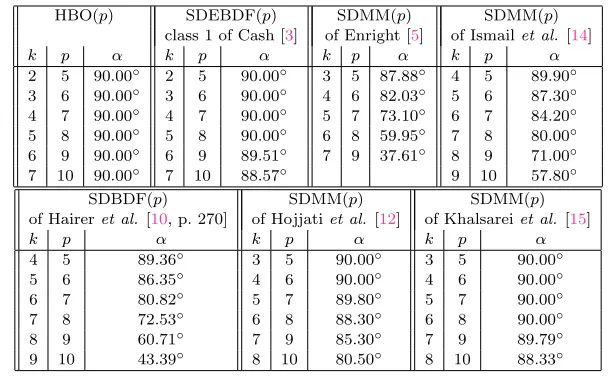
For each given step number k, Table 3 lists the α angles of A(α)-stability for HBO(5–10), SDEBDF(5–10) (class 1) of Cash [3], SDMM(5–9) of Enright [5], SDMM(5– 10) of Ismailet al. [14], SDBDF(5–10) of Hairer et al. [10, p. 270], SDMM(5–10) of Hojjati et al. [12] and SDMM(5–10) of Khalsarei et al. [15], respectively. It is seen thatαof HBO methods compare favorably withαof the considered methods of comparable orderp.

8. Controlling step size

The estimate∥yn−yen∥∞ and the current step hn are used to calculate the next step sizehn+1by means of formula [13]

hn+1= min

{

hmax, β hn

[

tolerance ∥yn−eyn∥_∞

]1/κ ,4hn

}

, (8.1)

with κ= pSCP+ 1 and safety factor β = 0.81. Here pSCP is the order of the step control predictor (SCP) (it is to be noted that the valueyenis obtained by the formula (2.3)).

The procedure to advance integration fromtn totn+1 is as follows.

(a) The step size,hn+1, is obtained by formula (8.1).

(15)

Table 3. For each given step numberk, the table lists the orderp,

theαangles ofA(α)-stability for the listed methods.

HBO(p) SDEBDF(p) SDMM(p) SDMM(p) class 1 of Cash [3] of Enright [5] of Ismailet al. [14]

k p α k p α k p α k p α

2 5 90.00◦ 2 5 90.00◦ 3 5 87.88◦ 4 5 89.90◦ 3 6 90.00◦ 3 6 90.00◦ 4 6 82.03◦ 5 6 87.30◦ 4 7 90.00◦ 4 7 90.00◦ 5 7 73.10◦ 6 7 84.20◦ 5 8 90.00◦ 5 8 90.00◦ 6 8 59.95◦ 7 8 80.00◦ 6 9 90.00◦ 6 9 89.51◦ 7 9 37.61◦ 8 9 71.00◦ 7 10 90.00◦ 7 10 88.57◦ 9 10 57.80◦

SDBDF(p) SDMM(p) SDMM(p)

of Haireret al.[10, p. 270] of Hojjatiet al.[12] of Khalsareiet al. [15]

k p α k p α k p α

4 5 89.36◦ 3 5 90.00◦ 3 5 90.00◦

5 6 86.35◦ 4 6 90.00◦ 4 6 90.00◦

6 7 80.82◦ 5 7 89.80◦ 5 7 90.00◦

7 8 72.53◦ 6 8 88.30◦ 6 8 90.00◦

8 9 60.71◦ 7 9 85.30◦ 7 9 89.79◦

9 10 43.39◦ 8 10 80.50◦ 8 10 88.33◦

(c) The coeﬃcients of predictors P2, integration formula IF, P3 and step control predictor P4 are obtained successively as solutions of systems (4.1), (4.3), (4.5) and (4.8).

(d) The valuesY2,Y3,yn+1, and eyn+1 are obtained by formulae (2.1) to (2.3). (e) The step is accepted if∥yn+1−eyn+1∥_∞is smaller than the chosen tolerance

and the program goes to (a) withnreplaced byn+ 1. Otherwise the program returns to (a) and a new smaller step sizehn+1 is computed.

9. _{Numerical results of comparing} L_{-stable methods}

Theerror at the endpoint of the integration interval (EPE, endpoint error) is taken in the uniform norm,

EPE ={∥yend−zend∥_∞},

whereyendis the numerical value obtained by the numerical method at the endpoint tendof the integration interval andzendis the “exact solution” obtained by MATLAB’s ode15swith stringent tolerance 5×10−14_.

The necessary starting values att1, t2, . . . , tk−1for HBO(p) were obtained by MAT-LAB’sode15swith stringent tolerance 5×10−14_.

Computations were performed on a PC with the following characteristics: Memory: 5.8 GB, Processor 0,1,. . . ,7: Intel(R) Core(TM) i7 CPU 920 @ 2.67GHz, Operating system: Ubuntu Release 11.04, Kernel Linux 2.6.38-12-generic, GNOME 2.32.1.

(16)

behaviour. We have chosen Problems3 and4 where the eigenvalues of the Jacobian matrix lie close to the imaginary axis, since it is problems of this type that cause major diﬃculties to many existing codes.

(1) The Oregonator equation describing Belusov-Zhabotinskii reaction [7].

Problem 1.

y₁′ = 77.27(y2+y1−8.375·10−6y21−y1y2), y1(0) = 1,

y₂′ = (y3−(1 +y1)y2)/77.27, y2(0) = 2,

y₃′ = 0.161(y1−y3), y3(0) = 3,

(9.1)

withtend= 360.

(2) The van der Pol’s equation [10, pp. 4–6], [12].

Problem 2.

y₁′ =y2, y1(0) = 2,

y₂′ =µ2[(1−y2₁)y2−y1], y2(0) = 0,

(9.2)

whereµ= 500 and withtend= 0.8.

(3) The stiﬀ DETEST problem B5 [6].

Problem 3.

y1′ =−10y1+αy2, y1(0) = 1,

y2′ =−αy1−10y2 y2(0) = 1,

y₃′ =−4y3 y3(0) = 1,

y₄′ =−y4 y4(0) = 1,

y₅′ =−0.5y5 y5(0) = 1,

y₆′ =−0.1y6 y6(0) = 1,

(9.3)

withα= 1000 andtend= 20.

(4) As above withα= 1500.

(5) A problem with large eigenvalues lying close to the imaginary axis [3].

Problem 4.

y1′ =−αy1−βy2+ (α+β−1)e−t y1(0) = 1,

y₂′ =βy1−αy2+ (α−β−1)e−t y2(0) = 1,

y₃′ = 1 y3(0) = 0,

(9.4)

withα= 1, β= 30, ﬁxed steph= 0.09 andtend= 20. The exact solution is

y1(t) =y2(t) =e−t, y3(t) =t.

(17)

Figure 1. log10(global error) versus log10hattn= 20 for the listed HBO(p) applied to problem (9.2) with µ = 1 over t ∈ [0,20] with constant stepsizes h.

−1.6 −1.4 −1.2 −1 −0.8 −0.6 −12

−10 −8 −6 −4 −2 0

HBO(9) HBO(10)

9.1. Numerical veriﬁcation of the order pof HBO(p). To show the relevance of the theoretical order of HBO(p), we have applied these methods with various constant stepsizeshon Problem (9.2) (van der Pol’s equation) withµ= 1 over t∈[0,20].

In Figure1, the global error ofy1andy2at tn= 20,

max{|y1,n−y1(tn)|,|y2,n−y2(tn)|}=O(hp),

is plotted in a log-log scale for the listed HBO(p) methods applied to problem (9.2) overt∈[0,20] with diﬀerent constant stepsizeshso that the curves appear as straight lines with slope p whenever the leading term of the global error is of order p. For HBO(p), the slopes of the straight lines which approximate the data in the least-squares sense are very close top, which conﬁrms the orders of the methods.

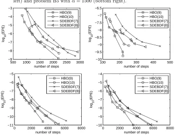
9.2. Comparing number of steps of selected L-stable HBO(p) and highly efficient existingL-stable methods. In our first tests, we numerically compare our most efficient methods HBO(p), p= 9,10 with the highly efficientL-stable methods which are the second derivative extended backward differentiation formulae, of class 1, of order 7 and 8 [3], denoted by SDEBDF(p),p= 7,8, on the basis of the EPE, endpoint error as a function of number of steps (NS). These classical SDEBDF(p) methods have been widely used to compare stiff ODE solvers.

Figure2depicts the graph of log₁₀(EPE) (vertical axis) as a function of number of steps (NS) (horizontal axis) for the considered test problems. Here, similar to Cash [4], we use also Problem3.

It is seen that, in general, HBO(p),p= 9,10, compare favorably with SDEBDF(p), p= 7,8.

Thenumber of steps percentage eﬃciency gain(NS PEG) of method 1 over method 2 is deﬁned by the formula (cf. Sharp [22]),

NS PEG = 100

[∑

jNS2,j

∑

jNS1,j −1

]

(18)

Figure 2. log10(EPE) (vertical axis) as a function of number of steps (NS) (horizontal axis) for Oregonator equation (top left), van der Pol’s equation (top right), problem B5 with α= 1000 (bottom left) and problem B5 with α= 1500 (bottom right).

500 1000 1500 2000 2500 3000 −9

−8 −7 −6 −5 −4 −3

number of steps

log

10

(EPE)

HBO(9) HBO(10) SDEBDF(7) SDEBDF(8)

100 200 300 400 500

−10 −9.5 −9 −8.5 −8 −7.5 −7 −6.5

number of steps

log

10

(EPE)

0 2000 4000 6000 8000

−11 −10 −9 −8 −7 −6 −5

number of steps

log

10

(EPE)

0 2000 4000 6000 8000

−10 −9 −8 −7 −6 −5 −4

number of steps

log

10

(EPE)

where NS1,j and NS2,j are the estimates of NS of methods 1 and 2, respectively, and j = −log10(EPE estimate). To compute NS2,j and NS1,j appearing in (9.5), we approximate the data (log10(EPE),log10(NS)) in a least-squares sense by MAT-LAB’spolyfit. Then, for chosen integer values of the summation index j, we take −log₁₀(EPE estimate) = j and obtain log₁₀(NS estimate) from the approximating curve, and ﬁnally the estimate of NS.

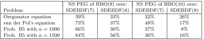
Table4lists the NS PEG of HBO(p),p= 9,10, over SDEBDF(p),p= 7,8, for the listed problems. It is seen that HBO(p),p= 9,10, win.

(19)

Table 4. NS PEG of HBO(p),p= 9,10, over SDEBDF(p),p= 7,8

for the listed problems.

NS PEG of HBO(9) over: NS PEG of HBO(10) over:

Problem SDEBDF(7) SDEBDF(8) SDEBDF(7) SDEBDF(8)

Oregonator equation 39% 33% 32% 26%

van der Pol’s equation 73% 37% 48% 17%

Prob. B5 withα= 1000 66% 30% 37% 8%

Prob. B5 withα= 1500 84% 56% 36% 16%

Table 5. CPU PEG of HBO(p), p= 9,10, over SDEBDF(p), p=

7,8 for the listed problems.

CPU PEG of HBO(9) over: CPU PEG of HBO(10) over:

Problem SDEBDF(7) SDEBDF(8) SDEBDF(7) SDEBDF(8)

Oregonator equation 17% 33% 5% -3%

van der Pol’s equation 73% 37% 26% -11%

Prob. B5 withα= 1000 65% 30% 28% -15%

Prob. B5 withα= 1500 96% 56% 33% -9%

The CPU percentage eﬃciency gain (CPU PEG) of method 1 over method 2 is deﬁned by the formula (cf. Sharp [22]),

(CPU PEG)i = 100

[∑

jCPU2,ij

∑

jCPU1,ij −1

]

, (9.6)

where CPU1,ij and CPU2,ij are the estimates of CPU time of methods 1 and 2, re-spectively, associated with problemi, and estimate of EPE = 10−j. The computation of CPU2,j and CPU1,j appearing in (9.6) is similar to the computation of NS2,j and NS1,j appearing in (9.5).

Table5 lists the CPU PEG of HBO(p),p= 9,10, over SDEBDF(p),p= 7,8, for the listed problems. It is seen that HBO(9) wins. For HBO(10), the NS PEGs for HBO(10) in Table4are positive and tend to be larger than the CPU PEGs in Table5 since the equations of the problems listed in Table4or5are relatively not expensive to evaluate. This would suggest that, when these equations become more expensive to evaluate, HBO(10) will be more eﬃcient in CPU time.

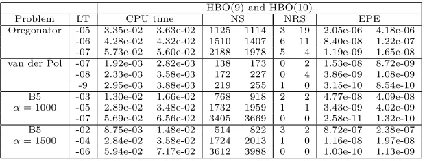
Table6compares the eﬃciency of HBO(9) and HBO(10) on 4 considered problems (9.1), (9.2), (9.3), (9.4) under listed LT = log₁₀(TOL). The comparison is based on CPU time in seconds,number of steps (NS),number of rejected steps(NRS) andend point error (EPE). It is seen that, to solve these 4 particular problems, in general, HBO(9) is more eﬃcient.

(20)

Table 6. For 4 considered problems (9.1), (9.2), (9.3), (9.4) and LT

= log₁₀(TOL), the table lists CPU time in seconds, number of steps (NS), number of rejected steps (NRS) and end point error (EPE) in corresponding left and right columns for HBO(9) and HBO(10), re-spectively.

HBO(9) and HBO(10)

Problem LT CPU time NS NRS EPE

Oregonator -05 3.35e-02 3.63e-02 1125 1114 3 19 2.05e-06 4.18e-06 -06 4.28e-02 4.32e-02 1510 1407 6 11 8.40e-08 1.22e-07 -07 5.73e-02 5.60e-02 2188 1978 5 4 1.19e-09 1.65e-08 van der Pol -07 1.92e-03 2.82e-03 138 173 0 2 1.53e-08 8.72e-09 -08 2.33e-03 3.58e-03 172 227 0 4 3.86e-09 1.08e-09 -9 2.95e-03 3.88e-03 219 255 1 0 3.15e-10 8.54e-10 B5 -03 1.30e-02 1.66e-02 768 918 2 2 4.77e-08 4.09e-08 α= 1000 -05 2.89e-02 3.48e-02 1732 1959 1 1 3.43e-09 4.02e-09 -07 5.69e-02 6.56e-02 3405 3669 0 0 2.58e-11 1.32e-10 B5 -02 8.75e-03 1.48e-02 514 822 3 2 8.72e-07 2.38e-07 α= 1500 -04 2.84e-02 3.58e-02 1724 2013 1 0 1.16e-08 1.97e-08 -06 5.94e-02 7.17e-02 3612 3988 0 0 1.03e-10 1.13e-09

Table 7. Error results obtained for the solution of Problem4(with α= 1, β = 30, ﬁxed step h= 0.09) as a function of step number k andt.

HBO methods SDEBDF methods

k= 6

t= 10.0 0.125×10−15 0.356×10−15 0.895×10−14 0.116×10−12

t= 15.0 0.157×10−17 0.382×10−17 0.520×10−13 0.143×10−12

t= 20.0 0.176×10−19 ₀_.₄₂₉_×₁₀−19 ₀_.₁₀₃_×₁₀−12 ₀_.₆₇₅_×₁₀−13 k= 7

t= 10.0 0.126×10−16 ₀_.₅₉₄_×₁₀−16 ₀_.₁₂₁_×₁₀−14 ₀_.₃₆₁_×₁₀−13 t= 15.0 0.620×10−16 ₀_.₅₃₀_×₁₀−16 ₀_.₁₃₉_×₁₀−12 ₀_.₁₆₄_×₁₀−12 t= 20.0 0.476×10−16 ₀_.₁₃₅_×₁₀−17 ₀_.₁₄₄_×₁₀−11 ₀_.₉₃₃_×₁₀−12

Jacobians have some large eigenvalues lying close to the imaginary axis. For this comparison, similar to Cash [3], we use Problem4.

Table7presents error results obtained for the solution of Problem4 (withα= 1, β = 30, ﬁxed step h= 0.09 suggested by Cash [3]) as a function of step number k andt. It is seen that HBO(p), p= 9,10, and SDEBDF(p), p= 9,10 remain stable for the integration of this problem.

(21)

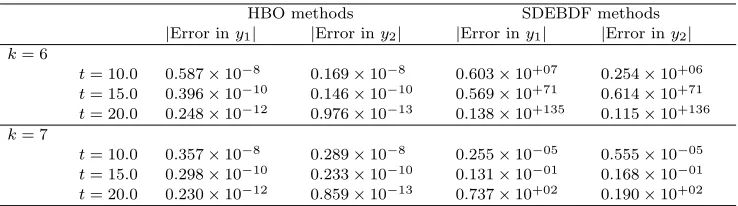
Table 8. Error results obtained for the solution of Problem4(with

α= 1, β = 42, ﬁxed step h= 1.00) as a function of step number k andt.

HBO methods SDEBDF methods

k= 6

t= 10.0 0.587×10−8 ₀_.₁₆₉_×₁₀−8 ₀_.₆₀₃_×₁₀+07 ₀_.₂₅₄_×₁₀+06 t= 15.0 0.396×10−10 ₀_.₁₄₆_×₁₀−10 ₀_.₅₆₉_×₁₀+71 ₀_.₆₁₄_×₁₀+71 t= 20.0 0.248×10−12 ₀_.₉₇₆_×₁₀−13 ₀_.₁₃₈_×₁₀+135 ₀_.₁₁₅_×₁₀+136 k= 7

t= 10.0 0.357×10−8 ₀_.₂₈₉_×₁₀−8 ₀_.₂₅₅_×₁₀−05 ₀_.₅₅₅_×₁₀−05 t= 15.0 0.298×10−10 ₀_.₂₃₃_×₁₀−10 ₀_.₁₃₁_×₁₀−01 ₀_.₁₆₈_×₁₀−01 t= 20.0 0.230×10−12 ₀_.₈₅₉_×₁₀−13 ₀_.₇₃₇_×₁₀+02 ₀_.₁₉₀_×₁₀+02

10. Conclusion

Second derivative multistep 3-stage Hermite–Birkhoﬀ–Obrechkoﬀ (HBO) methods of orderspwere considered. It is seen that HBO(p) areL-stable up to order 10.

Selected HBO(p) of order p, p = 9,10, compare positively with existing Cash modified extended backward differentiation formulae, SDEBDF(p),p= 7,8 in solving differential equations problems often used to test highly stable stiff ODE solvers.

HBO(p) of order p,p= 5,6, . . . ,10, are members of general step variable-order (VSVO) highly stable 3-stage k-step of order p = k+ 3 which appear to be promising highly stable stiﬀ ODE solvers in the light of the numerical results obtained in this paper.

11. _{Acknowledgment}

Thanks are due to the reviewer whose deep and extended comments contributed to substantially improve the manuscript. Thanks are also due to Mart´ın Lara for supplying the authors with his programs and sharing his experience. This work was supported in part by the Natural Sciences and Engineering Research Council of Canada.

Appendix A. Algorithms

Algorithm 1. This algorithm constructs Lk(i, i−1) entries of lower bidiagonal matrices Lk (applied toIF,Pℓ,ℓ= 2,3,4) as functions ofηj,j= 2,3, . . ..

Fork= 2 :kend, do the following iteration:

Fori=m:−1 :k+ 1, do the following two steps: Step (1) Lk(i, i−1) =−M(i, k)/M(i−1, k). Step (2) Forj=k:m, compute:

M(i, j) =M(i, j) +M(i−1, j)Lk(i, i−1),

wherekend=mℓ−1,ℓ= 1,2,3,4 for IF, Pℓ,ℓ= 2,3,4.

Algorithm 2. This algorithm constructs diagonal entriesUk(j, j)of upper bidiagonal matrices Uk(applied toIF,P2,P3andP4) as functions ofηj,j= 2,3, . . . .

Fork= 1 :kend, do the following iteration:

Forj=j0:−1 :k+ 1, do the following two steps:

(22)

Step (2) fori=k:j, compute

M(i, j) = (M(i, j)−M(i, j−1))Uk(j, j).

wherekendvalues are deﬁned in (5.6),j0=mℓ−1,ℓ= 1,2,3 for IF, P2, P3respectively andj0=m4for P4.

Algorithm 3. This algorithm solves the systems forPℓ,ℓ= 1,2,3inO(m2)operations. Given [η2, η3, . . . , ηp−3] and r = r(1 : m), the following algorithm overwrites r with the solution

u=u(1 :m) of the systemMu=r.

Step (1) The following iteration overwritesr=r(1 :m) withLm−1Lm−2· · ·,L2r: fork= 2,3, . . . , m−1, compute

r(i) =r(i) +r(i−1)Lk(i, i−1), i=m, m−1, . . . , k+ 1.

Step (2) This step forms the two matricesLmandLm+1which transformW1ℓ into the identity matrix Iℓ₌_L

m+1LmW1ℓ: this step computes the coeﬃcientsGm(i),i= 1,2, . . . , mused to form the two matricesLmandLm+1, whose nonzero entries are listed in Table2, as follows.

First setGm(1 :m),

Gm(1 :m) =M(1 :m, m).

The following computation overwritesGm(1 :m) withLm−1Lm−2· · · L2Gm(1 :m): fork= 2,3, . . . , m₋1, compute

Gm(i) =Gm(i) +Gm(i−1)Lk(i, i−1), i=m, m−1, . . . , k+ 1. Step (3) The following computation overwrites the newly obtainedrwithLm+1Lmr:

r(m) =r(m)/Gm(m), next, fork=m₋1, m₋2, . . . ,1,compute

r(k) =r(k)−Gm(k)r(m).

Step (4) The following iteration overwritesr=r(1 :m) withU1U2· · ·Um−2r: Fork=m−2, m−3, . . . ,1,compute

r(i) =r(i)Uk(i, i), i=k+ 1, k+ 2, . . . , m−1, r(i) =r(i)−r(i+ 1), i=k, k+ 1, . . . , m−2.

Algorithm 4. This algorithm solves the systems forP4 inO(m2)operations.

Given [η2, η3, . . . , ηp−3] and r = r(1 : m), the following algorithm overwrites r with the solution

u=u(1 :m) of the systemMu=r.

Step (1) The following iteration overwritesr=r(1 :m) withLm−1Lm−2· · ·L2r: fork= 2,3, . . . , m−1, compute

r(i) =r(i) +r(i−1)Lk(i, i−1), i=m, m−1, . . . , k+ 1. Step (2) The following iteration overwritesr=r(1 :m) withU1U2· · ·Um−1r:

Fork=m₋1, m₋2, . . . ,1,compute r(i) =r(i)Uk(i, i), i=k+ 1, k+ 2, . . . , m,

r(i) =r(i)−r(i+ 1), i=k, k+ 1, . . . , m−1.

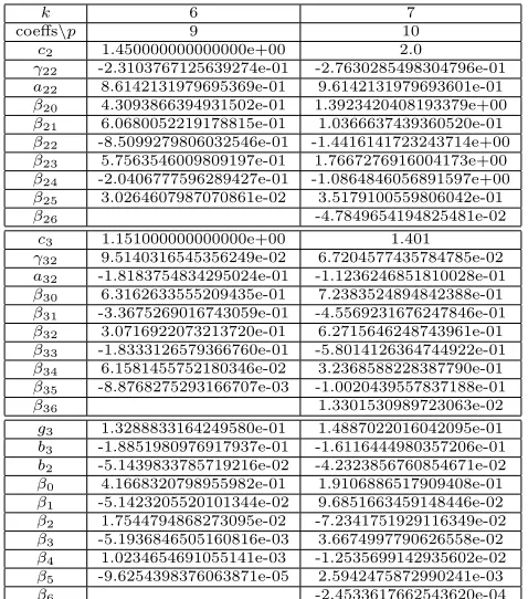
Appendix B. Coefficients of HBO(p), p= 9,10.

(23)

Table 9. Coeﬃcients of the implicit predictors Pi, i = 2,3 and of

the integration formulae of HBO(p),p= 9,10.

k 6 7

coeﬀs\p 9 10

c2 1.450000000000000e+00 2.0

γ22 -2.3103767125639274e-01 -2.7630285498304796e-01 a22 8.6142131979695369e-01 9.6142131979693601e-01 β20 4.3093866394931502e-01 1.3923420408193379e+00 β21 6.0680052219178815e-01 1.0366637439360520e-01 β22 -8.5099279806032546e-01 -1.4416141723243714e+00 β23 5.7563546009809197e-01 1.7667276916004173e+00 β24 -2.0406777596289427e-01 -1.0864846056891597e+00 β25 3.0264607987070861e-02 3.5179100559806042e-01

β26 -4.7849654194825481e-02

c3 1.151000000000000e+00 1.401 γ32 9.5140316545356249e-02 6.7204577435784785e-02 a32 -1.8183754834295024e-01 -1.1236246851810028e-01 β30 6.3162633555209435e-01 7.2383524894842388e-01 β31 -3.3675269016743059e-01 -4.5569231676247846e-01 β32 3.0716922073213720e-01 6.2715646248743961e-01 β33 -1.8333126579366760e-01 -5.8014126364744922e-01 β34 6.1581455752180346e-02 3.2368588228387790e-01 β35 -8.8768275293166707e-03 -1.0020439557837188e-01

β36 1.3301530989723063e-02

g3 1.3288833164249580e-01 1.4887022016042095e-01 b3 -1.8851980976917937e-01 -1.6116444980357206e-01 b2 -5.1439833785719216e-02 -4.2323856760854671e-02 β0 4.1668320798955982e-01 1.9106886517909408e-01 β1 -5.1423205520101344e-02 9.6851663459148446e-02 β2 1.7544794868273095e-02 -7.2341751929116349e-02 β3 -5.1936846505160816e-03 3.6674997790626558e-02 β4 1.0234654691055141e-03 -1.2535699142935602e-02 β5 -9.6254398376063871e-05 2.5942475872990241e-03

β6 -2.4533617662543620e-04

References

[1] A. Bj¨orck and T. Elfving,Algorithms for conﬂuent Vandermonde systems, Numer. Math.,21

(1973), 130–137.

[2] A. Bj¨orck and V. Pereyra, Solution of Vandermonde systems of equations, Math. Comp.,24

(1970), 893–903.

[3] J. R. Cash, Second derivative extended backward diﬀerentiation formulas for the numerical integration of stiﬀ systems, SIAM J. Numer. Anal.,18(1981), 21–36.

[4] J. R. Cash,A comparison of some codes for the stiﬀ oscillatory problem, Comput. Math. Appl.,

36(1998), 51–57.

[5] W. H. Enright, Second derivative multistep methods for stiﬀ ordinary diﬀerential equations, SIAM J. Numer. Anal.,11(1974), 321–331.

[6] W. H. Enright and J. D. Pryce,Two Fortran packages for assessing initial value methods, ACM Trans. Math., Software,13(1987), 1–27.

[7] J. Field and R. M. Noyes,Oscillations in chemical systems. IV: Limit cycle behavior in a model of a real chemical reaction, J. Chem. Phys.,60(1974), 1877–1884.

[8] G. Galimberti and V. Pereyra,Solving conﬂuent Vandermonde systems of Hermite type, Numer. Math.,18(1971), 44–60.