Joint Models for Spatial and Spatio-Temporal Point Processes

(1)

Scholarship@Western

Electronic Thesis and Dissertation Repository

11-21-2016 12:00 AM

Joint Models for Spatial and Spatio-Temporal Point Processes

Alisha Albert-Green

The University of Western Ontario

Supervisor

Dr. Charmaine Dean

The University of Western Ontario Joint Supervisor Dr. W. John Braun

The University of Western Ontario

Graduate Program in Statistics and Actuarial Sciences

A thesis submitted in partial fulfillment of the requirements for the degree in Doctor of Philosophy

Follow this and additional works at: https://ir.lib.uwo.ca/etd

Part of the Statistics and Probability Commons

Recommended Citation Recommended Citation

Albert-Green, Alisha, "Joint Models for Spatial and Spatio-Temporal Point Processes" (2016). Electronic Thesis and Dissertation Repository. 4306.

https://ir.lib.uwo.ca/etd/4306

This Dissertation/Thesis is brought to you for free and open access by Scholarship@Western. It has been accepted for inclusion in Electronic Thesis and Dissertation Repository by an authorized administrator of

(2)

In biostatistics and environmetrics, interest often centres around the development of

models and methods for making inference on observed point patterns assumed to be

generated by latent spatial or spatio-temporal processes. Such analyses, however, are

challenging as these data are typically hierarchical with complex correlation structures.

In instances where data are spatially aggregated by reporting region and rates are low,

further complications may result from zero-inflation.

In this research, motivated by the analysis of spatio-temporal storm cell data, we

gen-eralize the Neyman-Scott parent-child process to account for hierarchical clustering. This

is accomplished by allowing the parents to follow a log-Gaussian Cox process thereby

in-corporating correlation and facilitating inference at all levels of the hierarchy. A primary

focus for these data is to jointly model storm cell detection and trajectories. To do so,

storm cell duration, speed and direction are included in a marked point process

frame-work. The thesis also proposes a general approach for the joint modelling of multivariate

spatially aggregated point processes with the observed outcomes being zero-inflated count

random variables. For such models, we incorporate correlation between the random field

assumed to generate events and mean event counts. This is applied to lung and bronchus

cancer incidence by public health unit in Ontario and a study of Comandra blister rust

infection of lodgepole pine trees in British Columbia.

The key contributions from this thesis include the following: 1) developing a

spatio-temporal hierarchical cluster process that incorporates correlation at all levels of the

hierarchy, 2) joint modelling of a hierarchical cluster process and multivariate marks, 3)

extending the framework for the joint modelling of multivariate lattice data to enable

decomposition of the sources of shared spatial structure and 4) investigating aspects of

the partial misspecification of joint spatial structure for multivariate lattice data.

Keywords: joint modelling, spatio-temporal point processes, Neyman-Scott process,

log-Gaussian Cox process, zero-inflation, marked point processes, generalized additive

models, disease mapping, conditional autoregressive models.

(3)

This work was completed under the supervision of Dr. John Braun and Dr. Charmaine

Dean. All papers resulting from this thesis will be co-authored with Drs. Braun and

Dean.

(4)

This thesis would not have been completed without the generous support of my

super-visors, Charmaine Dean and John Braun. They have provide me with many interesting

avenues for research and I am thankful for their guidance and encouragement throughout

all aspects of this degree.

I would also like to express my gratitude to Doug Woolford for his continued support

and mentorship. He has always gone out of his way to listen and provide advice and for

that I am grateful.

I wish to thank Patrick Brown, Valerie Isham and Reg Kulperger for many useful

discussions related to point processes and Craig Miller for providing the storm cell data

and for answering all related questions. Thanks also to Cindy Feng for her insight related

to shared component models. I am grateful to my committee members Simon Bonner

and Francis Zwiers, in addition to Reg Kulperger and Craig Miller, for sharing their time

and expertise.

Many thanks are due to the graduate students in the Department of Statistical and

Actuarial Sciences, and in particular my fellow lab members, who have made my time at

Western so enjoyable.

Financial support provided by the Canadian Statistical Sciences Institute as well as

the Natural Sciences and Engineering Research Council of Canada and Queen Elizabeth

II scholarship programs is gratefully acknowledged.

Finally, I would like to thank my family for their unwavering love, support and

en-couragement.

(5)

Abstract i

Co-Authorship Statement ii

Acknowledgements iii

List of Figures vi

List of Tables ix

1 Introduction 1

1.1 Outline of Thesis . . . 3

2 Background 4 2.1 Point Processes . . . 4

2.2 Cox Processes . . . 6

2.2.1 Log-Gaussian Cox Processes . . . 6

2.2.2 Neyman-Scott Processes . . . 7

2.2.3 Parameter Estimation . . . 9

2.3 Marked Point Processes . . . 11

2.4 Aggregated Point Processes . . . 12

2.4.1 Zero-Heavy Data . . . 12

2.4.2 Random Effects . . . 14

2.4.3 Spline Smoothing . . . 16

3 A Spatio-Temporal Cluster Process for Modelling Storm Cells 19 3.1 Data Description . . . 20

3.2 A Point Process with Multiple Levels of Clustering . . . 22

3.2.1 Definition of Cluster Process Model . . . 23

3.2.2 Moment Properties . . . 24

3.2.3 Additional Assumptions . . . 26

3.2.4 Parameter Estimation . . . 27

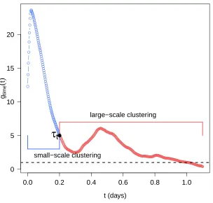
3.2.5 Identifying Multiple Levels of Clustering . . . 30

3.2.6 Confidence Intervals . . . 32

3.2.7 Goodness of Fit . . . 33

3.3 Application to Storm Cell Data . . . 34

3.3.1 Goodness of fit . . . 36

(6)

4 A Joint Model for a Hierarchical Cluster Process with Evolving Marks 43

4.1 Data Description . . . 44

4.2 Joint Models for Speed and Direction . . . 44

4.3 Spatio-Temporal Marked Point Process Model . . . 50

4.3.1 Marked Point Process . . . 50

4.3.2 Parameter Estimation and Inference . . . 53

4.4 Application to Storm Cell Trajectories . . . 55

4.4.1 Results . . . 55

4.4.2 Data Errors . . . 73

4.5 Discussion . . . 74

5 A General Framework for the Joint Modelling of Aggregated Spatial Point Patterns Subject to Clustering 77 5.1 Shared Component Models for Aggregated Point Patterns . . . 78

5.2 Shared Component Model Framework . . . 79

5.2.1 Model Description . . . 79

5.2.2 Parameter Estimation and Inference . . . 82

5.3 Applications . . . 83

5.3.1 Ontario Lung and Bronchus Cancer . . . 83

5.3.2 Comandra Blister Rust Infection of Lodgepole Pine Trees . . . 90

5.4 Misspecification of Spatial Structure . . . 96

5.4.1 Advantages of Including Between-Component Correlation . . . 97

5.4.2 Effect of Misspecification of Spatial Structure . . . 100

5.5 Discussion . . . 103

6 Future Work 106 6.1 A Joint Log-Gaussian Cox Process for Multivariate Aggregated Point Pat-terns . . . 107

6.2 A Composite Likelihood Approach to Parameter Estimation of a Spatio-Temporal Point Process . . . 107

6.3 Joint Estimation for Spatio-Temporal Point Processes with Evolving Marks108 Appendix A Supplementary Material for Chapter 3 110 A.1 Storm Cell Identification and Tracking Algorithm . . . 110

A.2 Verification of Campbell’s Theorem . . . 112

Appendix B Supplementary Material for Chapter 4 114

Appendix C Supplementary Material for Chapter 5 138

Bibliography 141

Curriculum Vitae 148

(7)

3.1 Initial location of storm cells detected in April 2003 at the Bismarck, North

Dakota radar station. . . 20

3.2 Locations of initial detection for April 2003 storm cells. . . 21

3.3 Locations of initial detection for May 2003 storm cells. . . 21

3.4 Locations of initial detection for June 2003 storm cells. . . 22

3.5 Locations of initial detection for July 2003 storm cells. . . 22

3.6 Locations of initial detection for August 2003 storm cells. . . 23

3.7 Empirical pair correlation function of the temporal projection process from April 2003. . . 31

3.8 Temporal and spatial empirical and fitted pair correlation functions for the hierarchical cluster process, the Neyman-Scott process and the log-Gaussian Cox process fit by month. . . 42

4.1 Storm cell duration, speed and direction from April 2003. . . 45

4.2 Storm cell duration, speed and direction from May 2003. . . 46

4.3 Storm cell duration, speed and direction from June 2003. . . 47

4.4 Storm cell duration, speed and direction from July 2003. . . 48

4.5 Storm cell duration, speed and direction from August 2003. . . 49

4.6 Fitted storm cell mean duration, speed and direction from April 2003. . . 60

4.7 Normalized quantile residuals for the duration, speed and direction com-ponents of the April 2003 mark models. . . 61

4.8 Fitted storm cell mean duration, speed and direction from May 2003. . . 63

4.9 Normalized quantile residuals for the duration, speed and direction com-ponents of the May 2003 mark models. . . 64

4.10 Fitted storm cell mean duration, speed and direction from June 2003. . . 66

4.11 Normalized quantile residuals for the duration, speed and direction com-ponents of the June 2003 mark models. . . 67

4.12 Fitted storm cell mean duration, speed and direction from July 2003. . . 69

4.13 Normalized quantile residuals for the duration, speed and direction com-ponents of the July 2003 mark models. . . 70

4.14 Fitted storm cell mean duration, speed and direction from August 2003. . 72

4.15 Normalized quantile residuals for the duration, speed and direction com-ponents of the August 2003 mark models. . . 73

5.1 Standardized incidence ratios of Ontario lung and bronchus cancer inci-dence for females and males. . . 90

(8)

bronchus cancer data. . . 91

5.3 Median posterior estimates and 95% credible intervals for the unstructured

random effects for females and males. . . 92

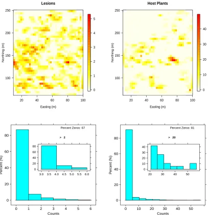
5.4 Level plots and histograms for lesion and host plant counts. . . 96

5.5 Linearly interpolated posterior median estimates of the shared random

effect. . . 97

5.6 Linearly interpolated independent random effects for lesions and host plants. 98

B.1 Estimated spatio-temporal partial effect on select days for the location

parameter in the duration component from April 2003. . . 115

B.2 Estimated spatial partial effect for the scale parameter in the duration

component from April 2003. . . 116

B.3 Estimated spatial and temporal partial effects for the location parameter

in the speed component from April 2003. . . 116

B.4 Estimated spatial partial effect for the scale parameter in the speed

com-ponent from April 2003. . . 117

parameter in the direction component from April 2003. . . 118

parameter in the duration component from May 2003. . . 119

parameter in the speed component from May 2003. . . 120

B.8 Estimated spatio-temporal partial effect on select days for the scale

pa-rameter in the speed component from May 2003. . . 121

parameter in the direction component from May 2003. . . 122

pa-rameter in the direction component from May 2003. . . 123

parameter in the duration component from June 2003. . . 124

parameter in the speed component from June 2003. . . 125

pa-rameter in the speed component from June 2003. . . 126

parameter in the direction component from June 2003. . . 127

pa-rameter in the direction component from June 2003. . . 128

parameter in the duration component from July 2003. . . 129

parameter in the speed component from July 2003. . . 130

(9)

parameter in the direction component from July 2003. . . 132

pa-rameter in the direction component from July 2003. . . 133

parameter in the duration component from August 2003. . . 134

parameter in the speed component from August 2003. . . 135

pa-rameter in the speed component from August 2003. . . 136

parameter in the direction component from August 2003. . . 137

(10)

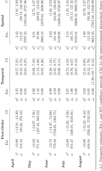
3.1 Parameter estimates and 95% confidence intervals for the spatio-temporal

hierarchical cluster process fit by month. . . 38

3.2 Parameter estimates and 95% confidence intervals for the spatio-temporal

Neyman-Scott process fit by month. . . 39

4.1 Summary from the four component model for storm cell trajectory in April

2003. . . 59

4.2 Summary from the four component model for storm cell trajectory in May

2003. . . 62

4.3 Summary from the four component model for storm cell trajectory in June

2003. . . 65

4.4 Summary from the four component model for storm cell trajectory in July

2003. . . 68

4.5 Summary from the four component model for storm cell trajectory in

August 2003. . . 71

5.1 Posterior median estimates and 95% credible intervals from the joint

spa-tial zero-inflated Poisson model for female and male cancer counts. . . 87

5.2 Proportion of spatial variability by model component and outcome. . . . 88

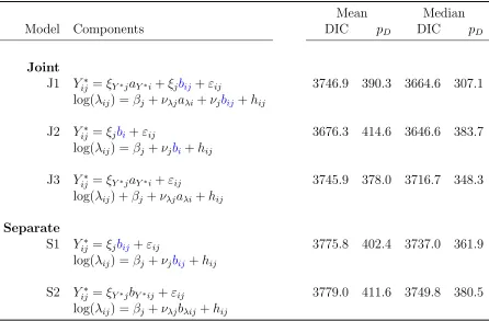
5.3 Comparison of deviance information criterion and effective number of

parameters for competing models in the analysis of Ontario lung and

bronchus cancer incidence. . . 88

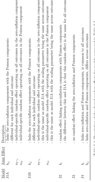
5.4 Description of the shared random effects for models compared in Table 5.3. 89

5.5 Posterior median estimates and 95% credible intervals from the joint

spa-tial zero-inflated Poisson model for lesions and host plants. . . 94

5.6 Comparison of deviance information criterion and effective number of

pa-rameters for competing models in the analysis of lesions and host plants. 95

5.7 Relative bias and relative root mean square error for scaling parameters

and variances from models J2, J3 and S1 at different levels of the variance

ratios. . . 101

5.8 Relative bias and relative root mean square error for scaling parameters

and variances from models J2, J3 and S1 at different levels of the variance

ratios when varying the neighbourhood structure. . . 104

C.1 Relative bias and relative root mean square error for intercept and

thresh-old parameters from the simulation study in Section 5.4.1. . . 139

(11)

(12)

Introduction

A point process is defined as a set of points or events that are generated stochastically and

distributed ind-dimensional space. A realization of a point process, referred to as a point

pattern, can arise in many fields of science, including medicine, meteorology, forestry,

ecology and seismology. In the most basic point process, a Poisson process, events occur

randomly and independently; this represents a standard against which other processes

may be compared. For example, if the occurrence of an event makes it more likely,

relative to a Poisson process, that another event will occur in a close neighbourhood, this

is referred to as a clustered process. Conversely, a process is considered to be regular if

the occurrence of an event makes it less likely that another event will occur. Examples

of clustered patterns include earthquake occurrences (e.g. Ogata, 1998) while in ecology,

plants that compete for resources may be regularly distributed (e.g. Yau and Loh, 2012).

Often events in a point process are indistinguishable other than by their location.

However, in some applications, additional characteristics can be recorded along with the

point. For example, in seismology, we may be interested in earthquake magnitude as well

as location. This extra information is referred to as a mark and the resulting point process

is called a marked point process. In some instances, such as when anonymity is a concern,

exact event locations are censored in space or space-time and instead counts aggregated

by region are recorded. In the spatial statistics literature, these data structures are

commonly referred to as lattice data (Cressie, 1993). Further, it is not uncommon that

when the underlying point process is clustered or non-randomly thinned there may be

(13)

more zeros than expected under the assumed distribution; this is referred to as

zero-inflation.

Methods for joint modelling of several outcomes measured on a single observation

have recently undergone rapid development, stemming from longitudinal studies with

the goal of understanding the relationship between an observed trajectory and a

time-to-event outcome (Diggle et al., 2008). In these types of analyses, the longitudinal and

survival random variables are assumed to depend on latent random effects common to

both outcomes. For point process data, joint modelling may refer to methods for

mul-tivariate point processes or to modelling a point and a mark process. In the context of

aggregated or lattice patterns, joint modelling via the so-called shared component model

is employed for increased power and facilitates the testing of a common spatial structure.

This thesis consists of three projects focussed on developing joint models for spatial

and spatio-temporal point processes. The first two projects are motivated by the analysis

of storm cell data from Bismarck, North Dakota. These types of data are known to

be hierarchically clustered with a group of storm cells referred to as a storm and a

storm system consisting of a cluster of storms (Mohee and Miller, 2010). Storm cells

are also dynamic and accordingly evolve over space and time. In the first project, we

develop a spatio-temporal hierarchical cluster process for the analysis of detected storm

cells that accounts for correlation and facilitates inference at all levels of the hierarchy.

We then extend this, in the second project, to jointly model storm cell detection and

movement through the use of multivariate marks corresponding to duration, speed and

direction. These models are expected to be used in simulations for understanding the

impact of stresses on power systems. The third project proposes a general framework

for the joint modelling of multivariate, zero-inflated spatial outcomes that arise due to

the aggregation of clustered or non-randomly thinned multivariate point processes. This

approach provides a clear conceptual interpretation to the generation of these random

variables and accounts for correlation between the random field generating the outcomes

and the mean of the observed outcomes. This joint model is applied to two data sets, the

first being an analysis of lung and bronchus cancer incidence in Ontario and the second

(14)

Columbia. The key contributions of this thesis are as follows:

1. Generalization of the Neyman-Scott parent-child process by allowing the parents to

follow a log-Gaussian Cox process thereby incorporating a hierarchical clustering

structure and facilitating inference at all levels of the hierarchy.

2. Extension of the hierarchical cluster process to a marked point process which

in-corporates multivariate and evolving marks to jointly model storm cell detection

and movement.

3. Development of a general framework for the joint modelling of multivariate spatially

aggregated point processes resulting in zero-inflated outcomes which incorporates

correlation between the random field assumed to generate events and mean count

outcomes and facilitates inference on the types of shared spatial structure across

all outcomes and components.

4. Investigation of aspects of partial misspecification of spatial structure for lattice

data.

1.1 Outline of Thesis

The rest of this document is organized as follows: Chapter 2 provides background on

as-pects of spatial and spatio-temporal point processes as they relate to the work contained

in this thesis. The development and application of the hierarchical cluster process for

storm cell data is provided in Chapter 3 and Chapter 4 extends this work by

incorporat-ing the multivariate storm cell trajectories in a marked point process. Chapter 5 then

shifts the focus to proposing a general framework for the joint modelling of multivariate

spatially aggregated point processes and investigating common aspects of

misspecifica-tion of the spatial structure in shared component models. We conclude in Chapter 6 by

(15)

Background

This chapter provides background on the key concepts employed throughout the thesis.

We begin with a brief introduction to point processes before building to Cox processes,

specifically the log-Gaussian Cox process and the Neyman-Scott process. We then

con-sider extensions to marked point processes and modelling concon-siderations for point

pat-terns aggregated on a lattice. Throughout this chapter we also highlight key pieces of

literature. Diggle (2003) and Illian et al. (2008) provide a thorough development of

spatial point processes. For temporal point processes Daley and Vere-Jones (2003) and

Daley and Vere-Jones (2008) are excellent references and for spatio-temporal patterns

Diggle (2014) is useful.

2.1 Point Processes

In this thesis, we are concerned with spatial (d = 2) and spatio-temporal (d = 3) point

processes. When describing these processes, we are often interested in the first- and

second-order intensities with the former related to the density of points and the latter

affiliated with patterns of clustering or regularity. The first-order intensity at x, λ(x),

corresponds to the probability of an event occurring in a small area containing x. In

the case of a homogeneous point process, λ(x) = λ. A point process is said to be

inhomogeneous ifλ(x) is not constant. The second-order intensity,λ(2)(x1, x2), represents

the probability of simultaneously getting points in small areas containing x1 and x2. If

(16)

λ(2)₍_x

1, x2) = λ(2)(x2 −x1) or λ(2)(x1, x2) = λ(2)(||x2 − x1||), with ||·|| denoting the

Euclidean norm, the corresponding point process is said to be stationary (translation

invariant) or isotropic (translation and rotation invariant), respectively.

Further summaries of second-order properties for stationary and isotropic point

pro-cesses include the K-function and the pair correlation function. The K-function, K(r),

is defined as λ−1_E_[_N

0(r)] where N0(r) represents the number of further events within a

distancer of an arbitrary event while the pair correlation function is

g(r) = λ

(2)₍_r₎

λ2 .

Ifr =||x2−x1||, this is defined as the probability of events occurring simultaneously near

x1 and x2 relative to what is expected from a Poisson process with first-order intensity

λ. Hence, for a Poisson process g(r) = 1, while g(r) > 1 and g(r) < 1 corresponds to

clustered and regular patterns, respectively. However, more complicated patterns also

exist. For example, Yau and Loh (2012) introduce a spatial point process that exhibits

clustering at small scales and regularity at large scales.

The Poisson process is the most basic form of a point process and is a situation

in which manipulation of the likelihood function is tractable. It may be expressed as

the product of two densities: the first corresponding to the Poisson R

Aλ(x)dx

distri-bution for the mean number of events on a bounded d-dimensional region A and the

second representing the density of the set of independent locations {xi, i= 1,2, . . . , N},

λ(xi)/

R

Aλ(x)dx. With this type of process the log-likelihood simplifies to

`(λ) =

N

X

i=1

log[λ(xi)]−

Z

A

λ(x)dx. (2.1)

For a homogeneous Poisson process, this function can be maximized analytically with

(17)

2.2 Cox Processes

Cox or doubly stochastic processes refer to a class of point processes in which the observed

point pattern is an inhomogeneous Poisson process conditional on a stochastic intensity,

Λ(x). They are defined by the following two postulates:

1. The intensity Λ(x) :x∈_Rd _{is a non-negative stochastic process.}

2. Conditional on Λ(x) = λ(x) :x∈_Rd _{, the observed pattern is an inhomogeneous}

Poisson process with intensity λ(x).

If the stochastic intensity is both stationary and isotropic, the resulting Cox process

possesses these properties. That is, if λ = E[Λ(x)] a process is said to be stationary

and if both stationary and isotropic λ(2)(r) =E[Λ(x1)Λ(x2)] where again r=||x2−x1||.

A weaker form of stationarity, known as second-order intensity reweighted stationarity,

has been developed for spatial (Baddeley et al., 2000) and spatio-temporal (Gabriel and

Diggle, 2009) processes where the assumption of a constant first-order intensity is relaxed.

As mentioned previously, the two specific forms of Cox processes that we focus on in this

thesis are the log-Gaussian Cox process (Møller et al., 1998) and the Neyman-Scott

process (Neyman and Scott, 1958).

2.2.1 Log-Gaussian Cox Processes

Log-Gaussian Cox processes are natural models for point patterns driven by

environmen-tal factors, for example non-infectious diseases. In this scenario, the resulting events are

due to exposure of observed and possibly unobserved environmental covariates. This is in

contrast to processes driven at least partially by interaction amongst the points, such as

infectious diseases. Furthermore, log-Gaussian Cox processes are completely

character-ized by their first-order intensity and their pair correlation function (see proof in Møller

et al., 1998).

Specifically, we assume that the observed pattern is driven by a Gaussian process

Z =Z(x) :x∈_Rd _where_E_[_Z₍_x_{)] =} _µ_{and Cov[}_Z₍_x

1), Z(x2)] =σ2ρ(x2−x1;φ) being

(18)

of clustering present with a larger value indicating greater clustering in the observed

pro-cess, while the scale parameter,φ, corresponds to the range of correlation in the Gaussian

process. Common covariance structures include Mat´ern, exponential and Gaussian. As

the name implies, the stochastic intensity generating the log-Gaussian Cox process, Λ(x),

is equal to exp{Z(x)}. This process has first-order intensity E[Λ(x)] = exp{µ+ 0.5σ2_}

and second-order intensityE[Λ(x1)Λ(x2)] = [exp{µ+ 0.5σ2}]2exp{σ2ρ(x2−x1;φ)}which

may be calculated directly from the properties of the log-normal distribution. The

pair correlation function for the log-Gaussian Cox process has the form g(x2 − x1) =

exp{σ2ρ(x2−x1;φ)}.

A convenient reparameterization of the process that we utilize in this thesis allows for

separation between the first- and second-order properties. As suggested in Diggle et al.

(2013) this may be obtained if we let Λ(x) = exp{β∗+Z(x)} with E[Z(x)] = −0.5σ2_.

In this case, E[exp{Z(x)}] = 1 and E[Λ(x)] = exp{β∗}=λ.

Covariates may be incorporated into the log-Gaussian process by replacing λ with

λ(x) =λ{ϕ(x);β}ifϕis a function of covariates indexed by location andβ= (β0, β1, . . . ,

βp)T resulting in a second-order intensity-reweighted stationary pattern. Log-Gaussian

Cox processes may also be employed for data where the region A is discretized into a

regular lattice. The number of events per region may then be modelled as Poisson random

variables (e.g. Diggle et al., 2013).

2.2.2 Neyman-Scott Processes

The Neyman-Scott process is a parent-child process commonly employed for modelling

clustered point patterns. It is defined as follows:

1. Parent points, P ={p1, p2, . . .} ∈Rd form a Poisson process with intensityλp.

2. Each parent generates an independent and identically distributed random number

of offspring, Nj, with mean α >0.

3. For the jth parent, the displacement of the offspring Xj = {x1j, x2j, . . . , xNjj}

relative to their parent is independent and identically distributed according to the

(19)

The observed pattern in this case consists only of the offspring. Typically, the

distri-bution generating the number of offspring is Poisson. For a planar point process, if the

density k(·) follows a bivariate normal distribution, this specification is referred to as a

modified Thomas process (Thomas, 1949) while a Mat´ern cluster process (Mat´ern, 1960)

results when the offspring are randomly scattered in a disc (d= 2) or ball (d= 3). More

generally, if d = 3 and k(·) = ks(·)kt(·), where ks(·) and kt(·) represent the spatial and

temporal displacement distributions, k(·) is said to be separable in space-time.

Com-monly, ks(·) is bivariate normal and kt(·) may be normal, exponential or half-normal

depending on the application. However, note that the case where kt(·) is normal

cor-responds to a scenario in which the offspring may appear prior to the arrival of their

parent. The displacement distribution is parameterized in terms of a standard deviation

parameter, ω; the radius, 2ω, represents the typical size of the cluster in space or time

(Wiegand et al., 2007).

Writing this as a Cox process, the distribution of the offspring conditional on the

parents is said to follow an inhomogeneous Poisson process with intensity ΛX|P(x) =

P

j:pj∈Pαk(pj, x;ω). Therefore, the Neyman-Scott process is a Cox process generated by

the stochastic intensity ΛX|P(x). As written, this process is stationary with unconditional

first-order intensityE[ΛX|P] =αλp, which is calculated by integrating out the unobserved

parents, and isotropic so long as the displacement distribution, k(·), is symmetric. The

corresponding second-order intensity and pair correlation function are

λ(2)(r) =α2λpk∗k(r;ω) +α2λ2p

and

g(r) = k∗k(r;ω)

λp

+ 1,

where ∗ is the convolution operator.

Extensions to second-order intensity reweighted stationarity are regularly employed

in order to incorporate covariates into the offspring distribution (e.g. Henrys and Brown,

(20)

2.2.3 Parameter Estimation

For a non-Poisson point process, evaluation of the likelihood treats the unobserved

in-tensity as missing data and utilizes Monte Carlo methods for maximization as it is not

available in closed form (Møller and Waagepetersen, 2004); this is typically

computation-ally prohibitive for Cox and cluster processes (Waagepetersen and Guan, 2009). With

log-Gaussian Cox processes specifically, integrated nested Laplace approximation may

be employed to quickly and accurately approximate the posterior marginal distributions

(Lindgren et al., 2011; Rue et al., 2009). For general stationary and isotropic spatial

point processes, parameter estimation is performed either by maximizing a composite

likelihood (e.g. Guan, 2006) or via minimum contrast estimation (e.g. Diggle, 2003). As

described in Guan (2006) the former derives a likelihood by summing log-likelihoods,

with each element being a valid marginal or conditional density. Specifically, they define

λ(2)₍_x

2−x1) R R

Sλ

(2)₍_x

2−x1)dx1dx2

as the joint distribution utilized for parameter estimation where S is a two-dimensional

region. Minimum contrast estimation is a non-parametric least squares approach to

parameter estimation which minimizes the discrepancy between an empirical function

of the data and a theoretical function based on the proposed process. Applied in the

context of point process modelling, the pair correlation function (e.g. Prokeˇsov´a and

Dvoˇr´ak, 2014) and theK-function (e.g. Henrys and Brown, 2009) are commonly utilized

for optimization. The remainder of this section focusses on the use of the pair correlation

function, which is employed throughout the thesis. This approach to estimating the

clustering parameters is conditional on the first-order intensity, which may be estimated

by solving an estimating equation that comes from differentiating an objective function,

such as the log-likelihood in Equation (2.1). As shown in Schoenberg (2005), estimates

based on this function are consistent even for non-Poisson processes. The clustering

parameters may then be estimated by minimizing

D =

Z rcorr

0

(21)

where g(u) is the theoretical pair correlation function and ˆg(u) is the empirical pair

correlation function, which in d dimensions is

ˆ

g(r) =

PN

i=1 P

j6=iκ(r− ||xi−xj||)vij

υ|A|λˆ2 . (2.2)

In the above, ˆλ is the estimated first-order intensity, κ is a kernel, such as the

Epanech-nikov, with bandwidth , vij is an edge correction factor (Gabriel, 2014) and υ =

2πd/2

Γ(d/2)r

d−1_. _{For a thorough overview of kernel density estimation, please see}

(Silver-man, 1998). Further, rcorr, termed the range of correlation, is the value above which

the empirical pair correlation function is equal to one. Finally, c is a constant which

stabilizes the variance inherent in ˆg(·). For minimum contrast estimation, the variance

of the empirical estimates increases withr. Therefore, the value of cis chosen to reduce

the influence of large values on the estimated parameters. Typically c= 0.5 for regular

patterns while a more severe transformation of c = 0.25 is suggested for clustered

pat-terns. For additional discussion on the choice of constant, we direct interested readers to

Diggle (2003). Although the composite likelihood approach has not yet been extended

to the spatio-temporal realm, the minimum contrast technique is known to be unstable

if extended directly to three dimensions (Prokeˇsov´a and Dvoˇr´ak, 2014). Accordingly,

parameter estimation for spatio-temporal point processes is still considered to be in its

infancy. Briefly, Onof et al. (2000) describe a spatio-temporal point pattern for

mod-elling rainfall that employs a generalized method of moments estimator. More recently,

the use of minimum contrast estimation for spatio-temporal cluster processes via the

lower dimensional spatial and temporal projection processes has been advocated (Møller

and Ghorbani, 2012; Prokeˇsov´a and Dvoˇr´ak, 2014).

Following this, obtaining confidence intervals for the parameters requires the use of

Monte Carlo methods, for example the parametric bootstrap (Davison and Hinkley, 1997)

or the non-parametric bootstrap (e.g. Braun and Kulperger, 1998; Loh, 2008; Loh and

(22)

2.3 Marked Point Processes

Sections 2.1 and 2.2 dealt with unmarked point processes only concerned with event

positions. However, sometimes points may also be characterized by additional variables

associated with the events, referred to as marks. That is, for a point process X in

A ⊂ _Rd_, _X

m = {[x, m(x)] :x∈X} is a marked point process where m(x) ∈ M is a

mark associated with the pointxin mark spaceM. An example of a well known marked

point process is the Neyman-Scott parent process. In Section 2.2.2, we defined the parent

process as a point process on _Rd×(0,∞). This can also be considered a marked point

process where the points are the parent process and the marks are the corresponding

number of offspring.

If we letX denote the unmarked point process andMdenote the marks, the goal for

a marked point process is to model the joint distribution of the events and the marks,

[X,M]. For example, the epidemic-type aftershock model (Ogata, 1998) considers data

on locations of earthquakes or aftershock as well as marks related to the corresponding

magnitude. However, if the point and marks processes are separable, it suffices to model

[X,M] = [X][M] where [X] and [M] denote the distribution of the point and mark

processes, respectively. That is, we can model the marks and points independently. For

spatial point processes, this amounts to employing point process techniques for modelling

the events and point-referenced methods for the marks. Tests for separability of points

and marks include Schoenberg (2004), for example. If X and M are not separable, the

dependence between these processes should be taken into account. This may also be done

through conditional analyses where [X,M] = [X][M | X] = [M][X | M]. The former

decomposition corresponds to a scenario in which the events are generated according to

a point process and the marks are modelled conditional on locations while the latter

corresponds to an analysis of the events conditional on the marks.

A marked point process may also be employed to reduce model complexity. For

example, a three-dimensional spatio-temporal point process can be fit as a spatial point

process with time as a mark or for modelling a non-simple point process in which there

(23)

be utilized for multivariate point patterns with a categorical mark for the type of event.

2.4 Aggregated Point Processes

As mentioned previously, point process applications are plentiful, and in these instances,

joint modelling techniques are often concerned with modelling the joint distribution of

the points and the marks. However, for applications in which anonymity is a concern, as

it commonly is for health administrative purposes with public health data, point patterns

may only be available in the form of aggregated counts. In fact, even given exact locations,

patterns may be discretized as likelihood-based techniques are then feasible for parameter

estimation. Joint models for discretized marked point processes have been successfully

fit. For example, Illian et al. (2012) fit a spatial log-Gaussian Cox process with two

spatially correlated marks in a shared component framework.

For aggregated patterns, joint modelling via shared component models is also

regu-larly utilized for multivariate outcomes hypothesized to have a common spatial structure

(e.g. Feng and Dean, 2012). A further complication is that zero-heaviness may arise as a

result of clustered patterns or due to non-random thinning. In what follows we introduce

methods for the analysis of zero-heavy count data as well as techniques employed to

account for spatial and spatio-temporal autocorrelation in these types of processes.

2.4.1 Zero-Heavy Data

Accounting for zero-heaviness in aggregated point patterns is traditionally done through

the use of zero-inflated models (e.g. zero-inflated Poisson regression models as originally

proposed by Lambert, 1992) or so-called hurdle models (e.g. Welsh et al., 1996).

How-ever, the choice of model is often guided by scientific objectives. In zero-inflated models,

zeros may arise either from the distribution for the counts or from the structural zero

component, the latter being represented by a distribution which takes on the value 0 with

probability one incorporated through a Bernoulli model, typically in a logistic framework.

This component is then mixed with a count distribution. The hurdle model can be

(24)

might equate to exceedance of the hurdle, and the second stage being the generation of

an outcome with positive support. For zero-heavy data, the hurdle corresponds to zero

and the conditional model would typically be a count distribution, truncated at zero.

Letting Y1, Y2, . . . , Yn denote n count random variables, if assumed to follow a

zero-inflated Poisson regression model,

Yi = 0, with probabilityπi

∼ Poisson(λi), with probability 1−πi

so

Yi =







0, with probability πi+ (1−πi)e−λi

k, with probability (1−πi)

e−λiλyi_i

yi! , k= 1,2, . . . .

The zero-inflation probability and the Poisson mean may be modelled as functions of

covariates, as follows:

%1(πi) = Giγ (2.3)

and

%2(λi) = Biβ (2.4)

where %1(·) and %2(·) are link functions for the zero-inflation and count components, Gi

and Bi are the covariate vectors for the ith observation incorporated into the two terms,

respectively, with γ= (γ0, γ1, . . . , γp1)

T _and _β_{= (}_β

0, β1, . . . , βp2)

T _{being the}

correspond-ing parameters. As advocated in Lambert (1992) and Hall (2000), the EM algorithm may

be employed for parameter estimation. However, if random effects are incorporated to

account for autocorrelated data or to link multivariate outcomes in a shared component

(25)

For the hurdle model,

Yi = 0, with probability 1−πi

∼ truncated Poisson(λi), with probabilityπi

such that

Yi =







0, with probability 1−πi

k, with probability πi

e−λiλyi_i

yi![1−e−λi], k = 1,2, . . .

where πi and λi can be modelled as functions of covariates, as shown in Equations (2.3)

and (2.4), respectively. In the hurdle framework, unlike the zero-inflated Poisson model,

it is fully efficient to estimate the two components separately and so standard iteratively

re-weighted least squares techniques may be employed to estimate parameters within each

component (Welsh et al., 1996). Zero-inflated distributions, however, are not constrained

to count data. For example, Li et al. (2011) employed a zero-inflated model for the

analysis of log-normal random variables with a point mass at zero.

2.4.2 Random Effects

Zero-heavy regression models are regularly employed for modelling autocorrelated data

whether they be spatial (e.g. Agarwal et al., 2002; Neelon et al., 2013; Recta et al., 2012)

or spatio-temporal (e.g. Tzala and Best, 2008; Richardson et al., 2006). If spatial data

are aggregated over a lattice, accounting for correlation is often accomplished through the

use of a conditional autoregressive random effect (Besag et al., 1991). These structures

can also be employed to approximate what is likely a correlation based on distances as

there may be computational advantages for largen. Additionally, distance-based effects

including the aforementioned Mat´ern or exponential structures may be utilized for spatial

or spatio-temporal point-referenced data or even lattice data based on the coordinates of

region centroids, for example.

In this thesis, when accounting for spatial correlation in lattice data, we employ

(26)

random effects for n regions and let W = (wii0) represent the spatial proximity matrix

wherewii0 = 1 if regionsiand i0 are neighbours (denotedi∼i0),w_ii0 = 0 otherwise. This

random effect is then specified through a series of conditional distributions, assumed to

be normally distributed, where

E[bi |bi0₆₌_i] =

1

wi+ X

i0_∼_i

bi0

denotes the conditional expectation with wi+ =P_i0wii0 and

Var[bi |bi0₆₌_i] =

σ_b2 wi+

is the conditional variance withσ2

b representing the variance. This random effect smooths

locally asE[b|bi0₆₌_i] is the average effect over the neighbours of region iand Var[b|b_i0₆₌_i]

is larger for regions with fewer numbers of neighbours. As shown in Besag (1974),

the vector b has a joint multivariate normal distribution where b ∼ MVN(0,Σ) and

Σ = σ2

b(D−W)

−1 _with _D _{= diag(}_w

1+, w2+, . . . , wn+). This formulation is termed the

intrinsic conditional autoregressive structure and, due to its conditional specification,

facilitates Markov chain Monte Carlo methods. Briefly, Markov chain Monte Carlo

tech-niques (Gelman et al., 2004) are a class of algorithms for sampling from a potentially

high dimensional target distribution, referred to as a posterior distribution, which may

be unavailable in closed form. For parameters, θ, if P(θ | Y) denotes the posterior

distribution and Y represents the random variables, then through Bayes theorem:

P(θ |Y) = R P(Y |θ)P(θ) P(Y |θ)P(θ)dθ

where P(Y | θ) is the likelihood and P(θ) represents the prior distribution. For the

conditional autoregressive random effect, Gibbs sampling, a type of Markov chain Monte

Carlo method in which parameters are estimated by sampling from their full conditional

distributions, is particularly convenient. However, for the intrinsic conditional

autore-gressive random effect specifically, because (D −W) is singular, this is an improper

prior and therefore a sum-to-zero constraint (i.e. Pn

(27)

iteration of the Markov chain Monte Carlo sampler (Eberly and Carlin, 2000).

2.4.3 Spline Smoothing

Splines provide an alternative approach to accounting for autocorrelation in spatial or

spatio-temporal data. While random effects are stochastic representations of smooth

functions, a spline is deterministic. However, Cressie (1993) showed that a thin plate

regression spline of order ms may be viewed as a realization of a Gaussian process

model with generalized covariance, C(r) ∝ r2ms−2_log(_r_{). Paciorek (2007) provides an}

overview of competing models used to account for spatial autocorrelation, including

splines. Splines will play an important role in some of the modelling methodology in

this thesis; for a thorough discussion of terminology and results, please see Wood (2006).

Specifically, splines are semi-parametric functions incorporated in linear or generalized

linear regression models as a flexible approach to accounting for non-linear covariate

effects (Wood, 2006; Hastie and Tibshirani, 1990). In our context, these effects would

include spatial coordinates and event times. The resulting model is referred to as a

generalized additive model.

Suppose Y1, Y2, . . . , Yn denotes random variables with conditional mean λi where

%(λi) =Biβ+ J

X

j=1

ϕj(xji).

Here, %(·) is the known link function,Bi are the covariates for theith observation which

are linearly related to%(λi),β = (β0, β1, . . . , βp)T are the corresponding coefficients and

ϕj is the jth smoother or piecewise polynomial for the covariate xji. Note that xji need

not be scalar; it may have two componentsxji = (x1ji, x2ji) or, for spatio-temporal data,

it may be the triplet xij = (x1ji, x2ji, x3ji) corresponding to two-dimensional space and

time. Suppose, for example, that xj is scalar and

ϕj(xj) = qj

X

k=1

ψjkηjk(xj), (2.5)

(28)

the basis function for the jth covariate at the kth knot and ψjk is the corresponding

coefficient. When utilizing splines, the number and location of knots needs to be carefully

selected. In a generalized additive model, this is accomplished by fitting a model with

more knots than required and adding a penalty term in the likelihood to control for

overfitting. Specifically, we maximize the following penalized log-likelihood

`pen(θ|y) = `(θ |y)− 1 2

J

X

j=1 ζj

Z

ψT_jΩj(xj)ψjdxj (2.6)

to estimate the parameters θ with θj corresponding to the elements of θ belonging to

thejth spline andΩj(xj) =

Pn

i=1η

00

j`(xji)η00j`0(x_ji) for`= 1,2, . . . , q_j and`0 = 1,2, . . . , q_j0.

This is performed conditional on the smoothing parameters,ζj, which controls the

trade-off between smoothness and fit. That is, if ζj = 0, ϕj(xj) would closely follow the data

while as ζj → ∞, ϕj(xj) becomes increasingly smooth. Smoothing parameter selection

is accomplished through generalized cross validation or unbiased risk estimation (Wood,

2006). Maximization of the likelihood may be accomplished through a penalized

itera-tively re-weighted least squares algorithm (Wood, 2006) or a backfitting algorithm (Rigby

and Stasinopoulos, 2005). One advantage of the latter approach is that, unlike in the

former, it does not require the response to be from within the exponential family.

Common forms of basis functions include tensor product splines, which are scale

invariant, and isotropic thin plate regression splines, which are rotation invariant. The

latter is recommended for spatial data if isotropy is a reasonable assumption while the

former may be useful if different amounts of smoothing for space and time are desired

with spatio-temporal data. Briefly, for thin plate regression splines, the smoother may

be written as

ϕ(x) =

q

X

k=1

ψ1kη1mdd(||x−x

∗

k||) + M

X

k=1

ψ2kη2k(x).

Here, x∗_krepresents the location of thekth knot,ψ₁ and ψ₂ contain unknown parameters

and η2k are linearly independent polynomials. If md is the order of the derivative

(29)

M = md+d−1

d

and

η1mdd(r) =







(−1)md+1+d/2

22_md−1_πd/2₍_m

d−1)!(md−d/2)!r

2md−d_log(_r₎_, _if _d _even

Γ(d/2−md)

22_md_πd/2₍_m

d−1)!r

2md−d_, _if _d _odd.

The corresponding penalty term is

Jmdd(ϕ) =

Z

· · ·

Z

Rd

X

m∗_d1+···+m∗_dd=md

md!

m∗_d₁!· · ·m∗_dd!

∂md_ϕ

∂xm

∗

d1

1 · · ·∂x

m∗_dd d

!2

dx1· · ·dxd

wherem∗_d₁, m∗_d₂, . . . , m∗_ddrepresents the order of the derivative for the respective covariate.

For a spatial smoother (d = 2), if we measure model flexibility by the squared second

derivative of the basis function, md = 2, M = 3, η21(x1, x2) = 1, η22(x1, x2) = x1 and

η23(x1, x2) =x2, then the basis function, ηmdd(r), is

1 8πr

2_log(_r_{) with penalty}

J22(ϕ) =

Z Z

∂2ϕ ∂x2 1

+ 2

∂2ϕ ∂x1∂x2

+

∂2ϕ ∂x2

2

dx1dx2.

For further discussion related to thin plate regression splines as well as various other

(30)

A Spatio-Temporal Cluster Process

for Modelling Storm Cells

This chapter deals with the development of models for possibly hierarchically clustered

spatio-temporal point patterns, motivated by the analysis of storm cell data.

On September 15, 1996 a severe thunderstorm brought down Manitoba Hydro

elec-tricity transmission line towers (Mohee and Miller, 2010). The accompanying winds lead

to numerous tower failures and an interruption in electricity supply from the

genera-tion plants in Northern Manitoba to the distribugenera-tion networks in North Dakota for the

two subsequent weeks; it caused a financial loss for Manitoba Hydro and was disruptive

to residents of Manitoba and North Dakota. This prompted research investigations led

by Manitoba Hydro on the modelling and prediction of the failure of transmission lines

caused by high intensity winds. Our focus here is understanding the clustering of storm

cells with hopes that this information could be utilized by power system operators who

monitor power flow on transmission lines. Accordingly, our goal for this chapter is to

de-velop a model for storm cell detection which facilitates inference on both storms (clusters

of storm cells) and storm systems (clusters of storms).

(31)

3.1 Data Description

The storm cell data used in this analysis are from the Bismarck, North Dakota radar

station which has a maximum detection range of 460 kilometers (km). Figure 3.1 displays

the location of this radar station with the storm cells from April 2003 identified. Scans

are performed every 4.5-6 minutes in precipitation mode and in clean-air mode they occur

in 10 minute intervals (Mohee and Miller, 2010).

Manitoba

Ontario

● ● ●●●●●

● ● ● ●

●

●_●_●

●

● ●

●

● ●

●

●●

● ● ●

● ●●

● ●

● _●●●●

● ●●● ●

●

● ● ●

●

●●●●● ● ●

●● _●

● ● ●●

●●● ●● ●

● ●

●● ●

●

● ●

● ● ● ●●●●

● ●●●

●● ● ●●_●

● ●

● ● ●

●

●●

● ● ● ●

● ● ●

● ●

●

● ● ●

●

●_●

● ●

●

● ● ●

●

●●

● ●

●

● ●●

● ●

●

● ●

●

● ●

● ● ● ●● ●

● ● ● ●

●

● ●

●●

● ● ●

●

● ●

● ●●

● ●

●

● _●

●

● ●

●

●● ●

● ●

● ● ● ●

● ●●

●

● ●

● ● ● ● ● ●

●

● ●

● ● ● ●

● ●

●

●●●

●

● ●

●

● ●

●

●● ●

●

● ●●

● ●

● ● ●

● ●

●

● ●●

● ● ● ● ●

● ●

● ● ● ● ● ●

● ● ●

● ●

●

● ●

● ● ● ●

● ●

●● ● ● ●

● ● ●

●

● ● ● ● ● ● ● ● ● ●

●

● ●

●

● ●● ●

●

● ● ● ● ●

●

● ● ●

● ●

●

● ● ●

● ● ● ●

●

● ●

●

● ●●●

● ●

● ● ●

● ●

●

● ● ●

● ●

●

● ● ●

●● ●

● ● ● ●

● ● ●

● _●

● ● ●

● ●

● ● ● ● ● ● ● ●

● ●

● ● ● ●

●●

● ●

●

● ● ●●

● ●

●

●●

●

● ● ●●

● ●

● ● ●

● ●● ● ●

● ●

●

● ●

●

● ●

●● ●●●

●

● ●●

●

●●

●

● ● ● ●

● ● ●_●● ●

● ●

● ● ● ● ● ●

● ● ● ● ●●●●●●

● ● ●● ● ●● ●● ●_●●●●●●

● ●

● ● ● ● ● ● ●

● ●

● ● ● ●

● ● ● ●●

●●● ●● ● ● ●

● ● ● ●

● ●

●●

● ● ●

● ●●

● ● ● ● ●●●_●●●●

● ● ●

● ●●

●● ●

● ● ●●_●_● ● ●●● ●

● ●

● ● ● ● ●● ● ●●● ● ● ● ● ●

● ●●

● ● ● ●

● ● ● ● ● ● ● ● ●

●

● ● ● ● ● ● ● ● ●_●

●●●●

●

●●

● ● ● ● ● ● ● ● ● ● ● ● ● ●

● ● ●

● ●

● ● ●

●

● ● ●

●

● ●

● ● ●

●

● ●

●

● ●

● ● ●

● ● ● ●

● ●

●

● ●

● ● ●

●● ●

●

● ●

●

● ●

● ● ● ● ●

●

● ●

●

● ●

●

● ●

●

● ●

●

● ● ●

●

● ●

●

● ●

●

● ● ●

●

● ●

●

● ● ●

● ●

●

● ●

●

●● ●

● ●

●

● ●

●

● ●

●

● ●

● ● ●

● ●

●

● ●

●

● ●●

●

● ●

●

●● ●

●●

●

● ●

● ● ●

●

● ●

●

● ● ● ●

●

● ●

●

● ●

●

● ●

●

● ●

●

● _●

● ● ●

● ●●

● ●

●●●●●

●Bismarck, North Dakota

Figure 3.1: Initial location of storm cells detected in April 2003 at the Bismarck, North Dakota radar station.

This analysis focusses on modelling the initial location of detected storm cells from

April 2003 - August 2003 which have been identified by a Doppler radar called Weather

Surveillance Radar-1988 and pre-processed according to the Storm Cell Identification

and Tracking algorithm outlined in Appendix A.1. For each storm cell, we have UTM

X and UTM Y coordinates of the mass-weighted centroids, precise to 10−4 km, and

time, measured in Julian days, accurate to within one second (U.S. Deparment of