Bilinear Time Delay Neural Network System for Humanoid Robot Software

(1)

Bilinear Time Delay Neural Network System for

Humanoid Robot Software

Fumio Nagashima

Fujitsu Laboratories Ltd.

Japan

1. Introduction

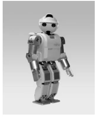
[image:1.595.215.376.411.608.2]

Recently there are many humanoid robot research projects for motion generation and control, planning, vision processing, sound analysis, voice recognition and others. There are many useful results for these elementary technologies by the effort of researchers. The humanoid robot HOAP (Fig.1, Fujitsu Automation) contributed these researchers and I also received a benefit from this robot for motion generation and control investigation. And in parallel, several researchers are working on formulation as a system based on these elementary technologies. The researchers in this area think how to integrate the system using many technologies and how to realize a suitable system for a certain purpose.

Figure 1. Humanoid robot, HOAP

There are two ways of thought to build the system, “top-down” and “bottom-up” (Minsky, 1990). Standing to “top-down” approach, they analyze the system regarding the total system balance and determine the interface between the elements from the total system demand. In this case, they must consider the efficiency to build the system and investigate the re-use

Source: Humanoid Robots: Human-like Machines, Book edited by: Matthias Hackel ISBN 978-3-902613-07-3, pp. 642, Itech, Vienna, Austria, June 2007

Open

Access

Database

(2)

technology. The typical example using this way is Humanoid Robot Project (HPR, Nakamura et al., 2001) in Japan. They analyze the tasks for each purpose, search common technologies and integrate these modules.

On another hand, “bottom-up” approach researcher try to design the small units and to make some rules for building the system using these units. In this area, there are some important results (Hawking, 2004). But there are very few results far less than ones based on “top-down” approach, because it’s difficult to make a small unit model and to make rules for all purposes needed for humanoid robots.

I show the design of a unit for ``bottom-up'' approach in this chapter. This design is based on an artificial neural network model. The concept of this design differs from ordinary neural networks. It’s for building the total software system of humanoid robot.

2. Neural Network

Because an artificial neural network is a mathematical model of biological neural network, it is expected to be a suitable model for building humanoid robot software system. But several researches on this area do not stand to this purpose. Many of them are related to new type mathematical problems, non-linear equation system. Such non-linearity is a part of reason for difficulty to build the large scale software system. The non-linearity must be in the connections, must not be in the neuron model itself. I give a reason and explain in last part of this section.

In this section, I outline the suitable model for building the large scale software system like humanoid robot one. The non-linearity scrambled out of neuron. First, I describe ordinary non-linear neural network shortly. It’s as a non-linear investigation tools.

2.1 Tool for Non-linear Research

The research of artificial neural network has a long history (Mcculloch, 1943). Some people believe this research area is a new activity for strong non-linearity and chaos related phenomena. Usually, the mathematical neuron models have the non-linearity, for example, sigmoid function. And the very useful learning method, back propagation (BP) is developed based on such a non-linearity. But it’s important to remind that the non-linear phenomena research and the neural network one are two different things.

The neural network using strong non-linearity has ups and downs. In the case of high dimensional problem, the strong non-linear network has an upper hand over linear ones (Barron, 1993). The invention of back propagation method may be a landmark event. This very useful method is applied to various kinds of problem. Some researchers use the threshold for a layered neural network (Nakano, 1972) and developed the method for association. It might be a promising step to brain function. In some cases, the non-linear factor has a superiority than the combination of linear factors (Barron, 1993). Some researchers also use the threshold for a neural oscillator (Kimura, 2003) and are interested in a phenomenon of limit cycle and entrainment between input signal and internal state. There researches demonstrate that the very small scale non-linear oscillator has functions of motion generation and adjusting itself to the variety of environment. It's amazing result. But this group suffers from the disadvantage of scale problem.

(3)

networks because there are strong interferences among networks even if each network is well constructed.

The artificial neural network is the mathematical model of biological neural network. Fundamentally speaking, an artificial neural network is a word categorized in a biologically inspired engineering and the non-linearity is a mathematical term. These are the words that are quite different research regions. All mathematical model based on biological neural network is an artificial neural network.

The research of engineering using non-linear effect is interesting and might be useful and proper biological model. But, we must give more attention to an alternative roll of artificial neural network, common notation for a large scale system.

Human's or animals' brain consist of biologically neural network. And these are very large scale systems. Therefore it is easy to get the idea that the artificial neural network can be applied to a large scale system.

2.2 Tool for Building the robot system

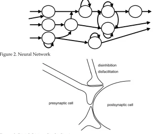
Generally a notation of neural network is simple. It consists of neurons and wirings as shown in Fig. 2. Such a uniform notation has a possibility for a common language of a huge variety of systems. For whole humanoid robot software system, we need many categories of systems, motion generation and control, vision processing, sound analysis and etc. I discuss the neural network model that is suitable for that sake of common language for all purpose of humanoid robot software system.

Figure 2. Neural Network

postsynaptic cell presynaptic cell

disinhibition

[image:3.595.114.425.396.667.2]

disfacilitation

(4)

Because the many engineering systems draw on linear operations, the goal system must be able to express the linear system for both algebraic and differential equation. There are many examples indicating this fact. PD control, the fundamental feedback control, outputs the value proportional to the input of position and velocity. Correlation calculation is for recognition of many things and it needs inner product between input and template. There operations are based on linear algebra. Moreover, PID control needs the integrator. The linear differential equation can output the some special functions, that is, triangle functions, polynomials and other eigen functions. In addition, the logical calculation is important for conditional process. As a result, the system must describe the following:

• linear algebra

• differential equation

• logical calculation

There are several formulations satisfying the above conditions. I use the following simple formula in the system.

¦

+

′

=

+

k j k j ijk k j k j ijk j j ij i i

i

y

C

y

C

y

C

H

y

dt

dy

, ,

)

(

ε

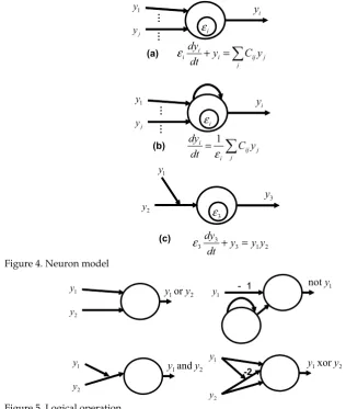
(1)

The left hand side represents the “delay”. The parameter

ε

_iis the “delay” scale.

y

_i

,

y

_j

,

y

_k are state quantity of neurons.

C

_ij

,

C

_ijk

,

C

_ijk

′

are connection weight, constant.

H

()

is a step function. Because all information transmission has delay in natural world, this formula is reasonable. The first term of right hand side is a linear connection, the second term is a bilinear connection and the third term is a digital bilinear connection. It becomes the linear equation putting

ε

_i

,

C

_ijk

,

C

_ijk

′

→

0

as follows:

¦

=

j

j ij

i

C

y

(2)

Adding

y

_ito right hand side as follows:

¦

+

′

+

=

+

≠ jk

k j ijk k j k j ijk i j j j ij i i i

i

y

C

y

C

y

C

H

y

dt

dy

, , ,

)

(

ε

(3)

It becomes an integrator for solving the differential equations.

It becomes a neuron keeping constant value, putting

ε

_i

→

∞

as follows:

0 )

(

1

1 lim

, ,

=

⎯→

⎯

°¿

°

¾

½

°¯

°

®

¸¸

¹

· ¨¨

©

§

′

+

=

+

¦

∞ →

dt

dy

y

H

C

y

C

y

C

y

dt

dy

i k j k j ijk k j k j ijk j j ij i i i i

i

ε

(4)

(5)

I should notice that this model has the similarities with fluid mechanics or something like that. Because Newtonian equation show the acceleration is exactly proportional to the external force, the motion equation of a infinitely small fluid particle is linear. But, The Navier-Stokes equation is a famous as linear equation system. In this case, the non-linearity also come from the interaction among particles. Most non-non-linearity is come from the interactions among a number of linear systems in natural world.

j

y

1

y

i

y

j j

ij i i

i

y

C

y

dt

dy

¦

=

+

ε

…

ε

i

j

y

1

y

i

y

j j

ij i i

y

C

dt

dy

¦

=

ε

1

…

ε

i

2 y

1

y

3

y

3

ε

2 1 3 3

3

y

dt

dy

=

+

ε

(a)

(b)

[image:5.595.109.426.224.598.2]

(c)

Figure 4. Neuron model

2 y

1 y

2 1ory

y

2 y

1 y

2 1andy

y

1

y ᧩᧭ noty1

2 y

1 y

2 1xory

y

-2

Figure 5. Logical operation

(6)

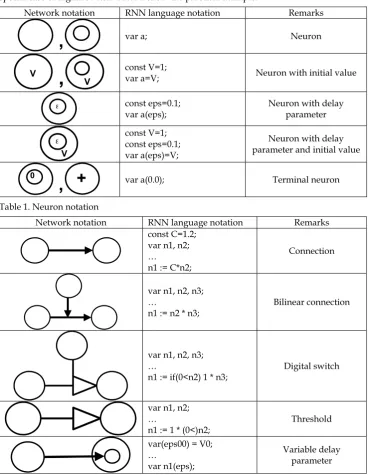
notation in this system. Table 2 show the connection notation. Table3 show the simple example of network. The digital switch is a digital bilinear connection. The threshold is a special case of digital switch. Table 4 show the practical example.

Network notation RNN language notation Remarks

,

var a; Neuron

,

V

const V=1;

var a=V; Neuron with initial value

ǭ const eps=0.1; var a(eps);

Neuron with delay parameter

ǭ

V

const V=1; const eps=0.1; var a(eps)=V;

Neuron with delay parameter and initial value

0

₊

[image:6.595.114.485.183.659.2]

,

var a(0.0); Terminal neuron

Table 1. Neuron notation

Network notation RNN language notation Remarks const C=1.2;

var n1, n2; …

n1 := C*n2;

Connection

var n1, n2, n3; …

n1 := n2 * n3;

Bilinear connection

var n1, n2, n3; …

n1 := if(0<n2) 1 * n3;

Digital switch

var n1, n2; …

n1 := 1 * (0<)n2;

Threshold

var(eps00) = V0; …

var n1(eps);

Variable delay parameter

(7)

Network notation RNN language notation Mathematical notation

ε

1 C

−

1 C

circuit cir1 { const C = 1.0; const eps = 0.1; var y1(eps) = 0.0; var y2(eps) = 0.0; y1 := 1.0 * y1 + C * y2; y2 := 1.0 * y2 – C * y1; }

1 2 2 2

2 1 1 1

Cy

y

dt

dy

Cy

y

dt

dy

−

=

+

=

+

[image:7.595.112.483.137.578.2]

ε

Table 3. RNN Example

Network Remarks

ε

1

1 _Integrator

Inner Product

Table 4. Practical RNN Example

Figure 6. Nueroma, the neural network editing and simulation tool

3. Basic Element Structure

There are many kinds of neural network until now. But the relationship among them is not discussed circumstantially. Especially, the researchers did not give much thought to the transformation between these. It’s not a problem if neural network is for a part of software system. But it’s not a good approach for building the whole software system.

) (t f

(8)

The purpose of the discussion in this chapter is to propose the neural network system for total robot software system. The goal of this discussion is the notation for dynamically growing neural network. For this goal, it is necessary to discuss the relationship between some models and the transformation from a typical neural network model to another. In this section, I discuss the important sub-networks and their relationship.

3.1 Linear Mapping, Correlation Calculation, Associative Memory

Linear transformation is a basic operation for proposed model. Using this operation I can build the correlation calculation network for estimate the similarity between an input and the template. Adding the threshold mechanism to this, the associative memory can be gotten (Nakano, 1972).

3.2 CPG

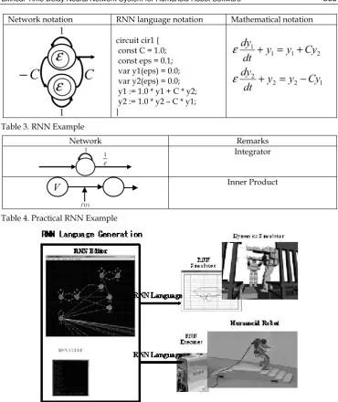
CPG is investigated by biological researcher (Grillner, 1985). It becomes known that a biological neural network can generate the non-zero output without input. This fact can be modelled using a successive linear transformation. I show the modification process using simple example. First, think the simple linear transformation, the above chart of Fig.7 can be describe by following equation:

»

¼

º

«

¬

ª

»

¼

º

«

¬

ª

−

=

»

¼

º

«

¬

ª

2 1 2 1

1

1 x

x

y

(4)

This equation is a kind of associative memory. Next, think the successive transformation of this equation as follows:

) ( 2 ) 1 ( 1 ) 1 ( 2 ) ( 2 ) ( 1 ) 1 ( 1 ) 0 ( 2 ) 0 ( 1

0

1

i i i i i i

y

+

=

−

=

+ +

+ (5)

This numerical sequence becomes as middle below chart of Fig.7. The cycle is just 6. Lastly, think the limitation of infinitely small time

i

and the following equation can be gotten:

1 2 2 1

,

y

dt

dy

y

dt

dy

=

−

=

(6)

Then,

0

1 1

₊

_y

₌

dt

dy

(7)

(9)

If it is assumed that this network is an associative memory, output of the network called a recall. Second network shows a successive recall using the same network. A broken line in a bottom graph shows this network output through time. Third network shows a continuous recall. A solid line in a bottom graph shows the continuous recall output. It is a CPG.

3.3 Bilinear, Parametric Resonance

Bilinear connection is a variable coefficient equation from the view of linear mathematics. Using the mechanism, the inner product, parametric resonance and some important calculation are realized.

3.4 Chaos

1

1 -1 1

1

x

2

x

1

y

2

y

1

1 -1

1 1

y

1

1 -1 1

) 1 ( 1

+

i

y

) 1 ( 2

+

i

y

) ( 1

i

y

) ( 2

i

y

2

y

ε

1

y

2

y

1

x

2

x

1

x

2

x

1

x

2

x

-1 -0.5 0 0.5 1

0 5 10 15 20

(a)

(b)

i

1

[image:9.595.188.406.281.657.2]

y

(10)

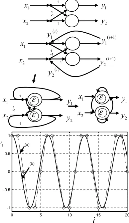
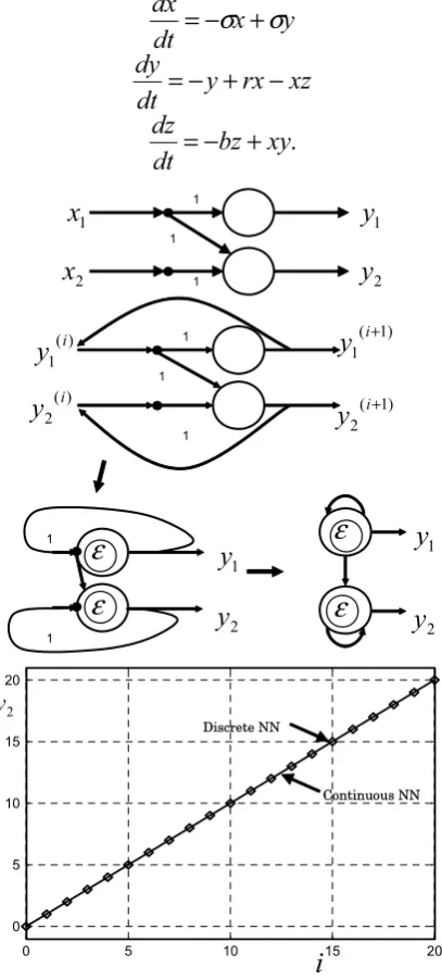
The low order chaos can be realized by a proposed system. But to keep the network understandable is very important to realize the large scale system. It is strongly recommended to use such a network carefully. Fig. 9 shows the network representing a Lorentz equation (Lorenz, 1963) as follows:

.

xy

bz

dt

dz

xz

rx

y

dt

dy

y

x

dt

dx

+

−

=

−

+

−

=

+

−

=

σ

(8)

1

1 1 1

x

2

x

1

y

2

y

1

y

1

1 1

) 1 ( 1

+

i

y

) 1 ( 2

+

i

y

) ( 1

i

y

) ( 2

i

y

2

y

ε

1

y

2

y

0 5 10 15 20

Discrete NN

Continuous NN

2

y

[image:10.595.195.399.209.661.2]

(11)

㧝㧝

㧝

b

−

1

−

σ σ

−

1

r

1

[image:11.595.213.380.149.243.2]

x y z

Figure 8. Neural network expression of Lorenz equation

4. Guideline for System Building

In this section, I discuss about the guideline for building the system. Usually the environments around a robot are very complicated. It is expected that a robot adjust itself for such environments. Mathematically these complexities are represented by non-linear equation systems. We can formulate an equation system in a few cases and cannot formulate that in many cases. Hence we need an algorithm to solve the non-linear equation system in the both given and unknown cases systematically.

4.1 Perturbation Method

In old days, astronomical scientist wanted to determine the orbit of planets. But it was hard because the governing equation system has non-linearity (Poincare, 1908) and they did not have a good calculation machine for numerical solution. Therefore, they developed perturbation method for getting the approximate solution of such a non-linear equation system.

If we can set up the equation system to determine the coefficient of neural network, we can use the perturbation techniques even if the system has non-linearity. A lot of techniques are developed (Hinch, 1991, Bellman, 2003). In this section, I show you a basic example using following equation(Hinch, 1991):

0

1

2

=

−

+

x

ε

(9)

This equation is analytical solved and has the solution as follows:

2

4

1

2

1 ε

+

±

−

=

x

(10)

For the explanation of perturbation technique, I assume

ε

is a small parameter and can be ignored in a first step as follows:

0

1

2

=

−

x

(11)

This equation is easily solved and has solution,

x

=

±

1

. This solution is a first approximation of the solution of Eq. (11) in a sense of perturbation technique.

ε

is small but not equal to zero, we can assuming

x

as follows:

+

=

2

2 1 0

)

(

ε

x

ε

x

ε

(12)

Substituting this equation into Eq.(11), we get the following sequential equations and solutions:

8

1

2 :

)

(

2

1

2 :

)

(

1

0

1 :

)

(

2 1

2 1 2 2

1 0

1 1

0 2

0 0

−

=

⎯→

⎯

+

−

=

−

=

⎯→

⎯

−

=

⎯→

⎯

=

−

x

O

x

O

x

O

ε

(13)

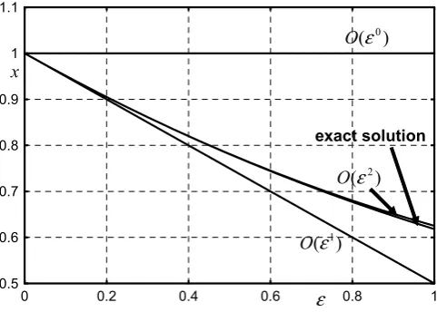
I choose the positive solution in the above. I show these approximate solutions and exact solution in Fig.10. It is noteworthy that it is good approximation even in the region,

ε

≈

1

.

0.5 0.6 0.7 0.8 0.9 1 1.1

0 0.2 0.4 0.6

_ε

0.8 1

x

)

(

ε

0

O

)

(

ε

2

O

)

(

ε

1

O

[image:12.595.176.417.297.469.2]

exact solution

Figure 9. Simple example of perturbation

In the case of differential equation system, the same concept is applied. For example, the following solution is a one of typical expansion for the equation having cyclic solution.

+

=

c

t

s

t

c

t

x

(

)

₀ ₁

cos

₁

sin

₂

cos

2

(12)

For the equation having non-cyclic solution, the expansion

t

,

t

2

,

t

3

,

is suitable assuming

t

is small. There are many types of expansion. See the references (Hinch, 1991, Bellman, 2003), for the variety of examples.

4.2 Numerical Perturbation Method

Unluckily if we cannot get the governing equation system, the same concept can be applied to solving the problem. I call this process “numerical perturbation method” and discuss in the section “Motion Generation and Control” and its references.

5. Applications

(13)

5.1 Forward Kinematics

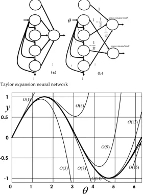
First of all, I show the basic problem in robotics, forward kinematics. The forward kinematics is the combination of triangle functions. Then, I start the discussion with the triangle function. To realize the triangle function in this system, Taylor-Maclaurin expansion is used as follows:

2 2 1 0

)

(

θ

c

θ

c

θ

y

=

+

(19)

where

y

is a arbitrary function of

θ

and

c

₀

,

c

₁

,

c

₂ are constants. I show the general neural network for such a expansion in Fig.11(a), and the concrete example,

sin

θ

(Eq.(20)) in Fig.11(b).

…

(a) _(b)

! 2 1

−

1

! 4 1

1 1

1

θ

! 3 1

−

ᇫ

θ

cos

ed approximat

θ

sin

[image:13.595.154.435.277.659.2]

ed approximat

Figure 11. Taylor expansion neural network

) 1 (

O

) 3 (

O

) 5 (

O

) 7 (

O

) 9 (

O

) 11 (

O

) 13 (

O

) 15 (

O

θ

y

-1 -0.5 0 0.5 1

0 1 2 3 4 5 6

(14)

+

−

+

−

+

−

=

3 5 7 9 11

!

11

1 !

9

1 !

7

1 !

5

1 !

3

1 sin

)

(

θ

y

(20)

Fig.12 shows the result of such an approximation. In this figure, the heavy line is

sin

θ

, the other lines are approximate solution,

O

(

n

)

represents

O

(

θ

n

)

solutions. In this case,

)

17 (

O

solution is drawn, but it’s just on the exact solution’s line.

5.2.1 Analytical Method

In this sub-section, I show illustrative case. The simple arm (Fig.13) kinematics solution can be solved analytically as follows:

)

sin(

sin

))

sin(

sin

(

sin

))

sin(

sin

(

sin

3 2 2 2 1 3 2 2 2 1 1 3 2 2 2 1 1

θ

+

=

+

=

+

=

l

z

l

y

l

x

(21)

The neural network representing this equation is as Fig. 14

5.2.2 Numerical Method

The kinematics problem is a fitting problem for multivariable polynomial. Then this problem is determining coefficients problem assuming the position is as follows:

+

¸

¹

· ¨

©

§

• +

¸

¹

· ¨

©

§

• +

=

(

0 )

!

2

1 )

0 (

)

0 (

)

(

X

ș

X

ș

X

ș

X

d

δ

(22)

[image:14.595.230.363.484.667.2]

To determine coefficients problem is calculation follwing values from the actual measurements.

x

y

z

1

θ

2

θ

3

θ

2

l

1

l

(15)

… … ! 3 1 − 1 ! 5 1 ! 7 1 − 1 1 1 1 1 θ … … ! 3 1 − 1 ! 5 1 ! 7 1 − 1 1 1 1 1 θ … … ! 3 1 − 1 ! 5 1 ! 7 1 − 1 1 1 1 1 θ

x

y

z

1

θ

2

θ

3

θ

…… …

Figure 14. Kinematics neural network

,

2 2 l k j i k j i j i i

d

x

d

x

d

dx

x

θ

[image:15.595.121.484.154.659.2]

θ

(23)

Fig. 15 show the growing neural network in this process.

1

θ

2

θ

3

θ

x

y

z

(a) 1st_{order terms of the Polynomial}

(b) A part of 2nd _{order terms of the Polynomial}

x

1

θ

2

θ

… …

x

1

θ

2

θ

(c) A part of 3rd _{order terms of the Polynomial}

…

[image:15.595.154.434.436.646.2]

(16)

5.2 Inverse Kinematics

In this sub-section, I discuss the inverse kinematics problem. In this problem, the solution has an inverse trigonometric function.

5.2.1 Analytical Method

The inverse kinematics of the arm (Fig.13) has 4 type solutions. In this sub-section, I only discuss following solution. The other solutions can be considered in the similar way.

(

)

(

)

[

]

α

θ

+

=

¿

¾

½

¯

®

+

−

+

=

− − −

r

z

l

z

y

x

l

y

x

1 2

2 2 2 1 2 2 2 2 1 1 3

1 1

cos

2

1 cos

tan

(24)

In the similar fashion as the forward kinematics, there is a convergence radius problem of the Taylor expansion of the term,

1 /

y

,

tan

−1

(

x

/

y

),

cos

−1

(

z

/

r

)

. It can be avoidable using the concept of analytical continuation. For example, because the function,

tan

−1

(

x

/

y

)

has the singular points at

±

i

, the expansion near

x

/

y

=

0

breaks down near

±

1

. Fig.16 show the example of region splitting for

tan

−1

(

x

/

y

)

. Such techniques keep a high accuracy for wide range. Fig. 17 shows a part of the neural network using such techniques. It includes the digital switch neuron.

-1.5 -1 -0.5 0 0.5 1 1.5

-2 0 2 4 6 8 10 12 14 16

0

3 1

3

6 y

x

/

[image:16.595.166.428.438.656.2]

θ

Figure 16. Approximate solution of

y

x

1

tan

−

(17)

5.2.2 Numerical Method

If we do not have the information of arm, the above technique can be applied numerically. In this case, the neural network has the some polynomials with digital switch (Fig.17).

[image:17.595.164.423.191.355.2]

… … ! 3 1 − 1 ! 5 1 ! 7 1 − 1 1 1 1 1 θ

x

y

z

1

θ

2

θ

3

θ

…

y 1 y x 1 tan− ! 3 1 − 1 ! 5 1 ! 7 1 − 1 1 1 1 1 θ ! 3 1 − 1 ! 5 1 ! 7 1 − 1 1 1 1 1 θ ! 3 1 − 1 ! 5 1 ! 7 1 − 1 1 1 1 1 θ ! 3 1 − 1 ! 5 1 ! 7 1 − 1 1 1 1 1 θ

…

Figure 17. A part of inverse kinematics neural network

5.3 Motion Generation and Control

There are many references about the motion generation and control using this system. See references(Nagashima, 2003). Fig. 18 show the example of growing neural network for motion.

ε

Output Neuron

(a) Cyclic motion

(b) Non-cyclic motion

[image:17.595.147.437.449.645.2]

(18)

ε

0

0 ε

0

0 …

…

Joint

neurons

ε

Smoothing

neurons

ε

[image:18.595.144.444.153.664.2]

…

Figure 19. An example of motion neural network

1

ε

2

ε

Gyro sensor signal

01

C

02

C

21

C C12

11

C

22

C

13

C

23

C

0

ε

+

[image:18.595.145.436.158.349.2]

Feedback signal

Figure 20. An example of feedback neural network

[image:18.595.171.424.480.658.2]

(19)

Fig. 19 shows the neural network example for real motion. Fig. 20 shows the feedback neural network for stabilize the upper body of humanoid robot. Fig. 21 shows the HOAP, humanoid robot for experiment of walk.

5.4 Sound Analysis

It is popular that the Fourier transformation (FT) is applied to the pre-processing of a sound analysis. Usually neural network for sound analysis uses the result of this FT. But it's unnatural and wrong in a sense of neural network as a total system basis. In this section, I discuss the problem of the transformation of signal.

Proposed model can compose the differential equation for triangle functions as shown in previous section. I call this network CPG. Putting the signal to the neuron and wire of this CPG, this becomes the resonator governed by the following equation,

ε

signal

ε

sound signal ( raw data)

(a)

(b)

+

0

C

−

C

₀

1

C

2

C

1

y

2

y

3

y

b

−

1

[image:19.595.152.479.282.623.2]

s

Figure 22. Central Pattern Recognizer (CPR)

(

s

)

y

s

dt

dy

dt

y

d

f

m

δ

ω

β

+

=

+

1 2 ₁

2 1 2

1

(25)

dt

dy

y

1

2

=

−

ω

(26)

2 2 2 1

3

y

=

+

(27)

where

s

is input signal,

β

,

ω

,

δ

_m

,

δ

_f are constants determined by connection weights,

2 1

,

y

(20)

call this network Central Patten Recognizer (CPR). Using a number of this network, it is possible to create the network which function is very similar to FT. Fig.23 shows the elements of cognitive network, CPR. Fig.24 shows the output of this network and it is a two-dimensional pattern. The sound analysis problem becomes the pattern recognition of this output. The pattern recognition problem is solved by the fitting function problem similar to kinematics problem.

…

0

A

1

A

2

A

n

A

…

[image:20.595.199.396.227.407.2]

…

Figure 23. Sound analyzing neural network

Figure 24. Example of sound analyzing results using CPR

n

A

1

[image:20.595.167.405.430.658.2]

(21)

5.5 Logical Calculation

Logical calculation is a basic problem for neural network in old days. Especially, exclusive-OR problem offer the proof that perceptron cannot solve the non-linear problem. In this section, I show examples which can solve the nonlinear logic problem using proposed system. Fig.5 shows the basic logical calculations, (or, and, not, xor). Fig.25 shows the simple application network. It shows the half adder which is the lowest bit adder circuit in an accumulator.

y

x

c

s

1

−

1

−

[image:21.595.137.452.235.420.2]

εε

Figure 25. Half adder

5.6 Sensor Integration

The goal of this method is an integration of software system. The fusion of sensor problem is a well-suited application of this model. The concept of an associative memory is known as the introduction to a higher cerebral function. Especially, autocorrelation associative memory is important (Nakano, 1972). This concept can restore the noisy and muddy information to original one. Proposed model can work out this concept through the multiple sensing information. This fact is very important. Proposed model can treat the all sensing data evenly. In a similar fashion, the sensing result information at any levels can be treated evenly.

6. Conclusion

In this chapter, I describe the neural network suitable for building the total humanoid robot software system and show some applications. This method is characterized by

• uniform implementation for wide variety of applications

• simplicity for dynamically structure modification

The software system becomes flexible by these characteristics. Now, I’m working on the general learning technique for this neural network. There is a possibility free from NFL problem (Wolper, 1997).

(22)

7. References

Barron, A,(1993). Universal Approximation Bounds for Superpositions of a Sigmoidal Function, IEEE Trans. on Information Theory, IT-39, pp.930-944.

Bellman, R,(2003). Perturbation Techniques in Mathematics, Engineering and Physics, Dover Publications, Reprint Edition, June 27.

Fujitsu Automation. http://jp.fujitsu.com/group/automation/en/.

Grillner, S, Neurobiological Bases of Rhythmic Motor Acts in Vertebrate, Science 228, 143-149 Grune, D and Ceriel J.H.Jacobs, Parsing Techniques,(1991). A Practical Guide, Ellis Horwood Ltd. Hawking, J and Blakeslee, S, (2004). On Intelligence, Times Books

McCulloch, W. and Pitts, W. ,(1943). A Logical Calculus of the Ideas Immanent in Nervous Activity, Bulletin of Mathematical Biophysics, 5, pp. 115-133

Hinch, E.J., etc., (1991). Perturbation Methods, Cambridge University Press, October 25. Kimura, H, Fukuoka, Y. and Cohen A.H.,(2003). Biologically Inspired Adaptive Dynamic

Walking of a Quadruped Eobot, in 8th International Conference on the Simulation of Adaptive Behavior, 2003, pp. 201-210

Lorenz, E.N., (1963). Deterministic nonperiodic flow, J. Atmos. Sci., 20, 130

Minsky, M. (1990). Logical vs. Analogical or Symbolic vs. Connectionist or Neat vs. Scruffy,

Artificial Intelligence at MIT, Vol.1, Expanding Frontiers, MIT Press

Nagashima, F, (2003). A Motion Learning Method using CGP/NP, Proceedings of the 2nd International Symposium on Adaptive Motion of Animals and Machines, Kyoto, March, 4-8

Nagashima, F, (2004). - NueROMA -, Homanoid Robot Motion Generation System, Journal of the Robtics Society of Japan, Vol.22, No.2, pp.34-37 (in Japanese)

Nagashima, F ,(2006). A Bilinear Time Delay Neural Network Model for a Robot Software System,Journal of the Robotics Society of Japan, Vol.24, No.6,pp.53-64 (in Japanese) Nakamura, Y. et al. (2001). Humanoid Robot Simulator fot the METI HRP Project, Robotics

and Autonomous Systems, Vol.37, pp.101-114

Nakano, K., (1972). Associatron – A Model of Associative Memory, IEEE Trans. on Systems Man and Cybernetics, SMC 2, pp. 381-388

Poincare,(1908). Science et Methode

Bellman, R, (2003). Perturbation Techniques in Mathematics, Engineering and Physics, Dover Publications; Reprint Edition, June 27

Rumelhart, D. E. , Hinton, G. E. and McCelland, J. L. (1986). A General Framework for Parallel Distributed Processing, In D.E.Rumelhart and J.L.McClelland(Eds.),:

Parallel Distributed Processing: Explorations in the Microstructure of Cognition, Cambridge, Ma, MIT Press, 1, pp. 45 - 76

Shan, J, Nagashima, F. (2002). Neural Locomotion Controller Design and Implementation for Humanoid Robot HOAP-1, RSJ conference , 1C34

(23)

Edited by Matthias Hackel

ISBN 978-3-902613-07-3 Hard cover, 642 pages

Publisher I-Tech Education and Publishing Published online 01, June, 2007

Published in print edition June, 2007

InTech Europe

University Campus STeP Ri Slavka Krautzeka 83/A 51000 Rijeka, Croatia Phone: +385 (51) 770 447 Fax: +385 (51) 686 166 www.intechopen.com

InTech China

Unit 405, Office Block, Hotel Equatorial Shanghai No.65, Yan An Road (West), Shanghai, 200040, China

Phone: +86-21-62489820 Fax: +86-21-62489821

In this book the variety of humanoid robotic research can be obtained. This book is divided in four parts: Hardware Development: Components and Systems, Biped Motion: Walking, Running and Self-orientation, Sensing the Environment: Acquisition, Data Processing and Control and Mind Organisation: Learning and Interaction. The first part of the book deals with remarkable hardware developments, whereby complete humanoid robotic systems are as well described as partial solutions. In the second part diverse results around the biped motion of humanoid robots are presented. The autonomous, efficient and adaptive two-legged walking is one of the main challenge in humanoid robotics. The two-legged walking will enable humanoid robots to enter our environment without rearrangement. Developments in the field of visual sensors, data acquisition, processing and control are to be observed in third part of the book. In the fourth part some "mind building" and communication technologies are presented.

How to reference

In order to correctly reference this scholarly work, feel free to copy and paste the following:

Fumio Nagashima (2007). Bilinear Time Delay Neural Network System for Humanoid Robot Software, Humanoid Robots, Human-like Machines, Matthias Hackel (Ed.), ISBN: 978-3-902613-07-3, InTech, Available from: