A decomposition heuristics based on multi-bottleneck machines for large-scale job shop scheduling problems

JIEM, 2014 – 7(5): 1397-1414 – Online ISSN: 2013-0953 – Print ISSN: 2013-8423 http://dx.doi.org/10.3926/jiem.1206

A Decomposition Heuristics based on Multi-Bottleneck

Machines for Large-Scale Job Shop Scheduling Problems

Yingni Zhai

1

, Changjun Liu

1

, Wei Chu

1

, Ruifeng Guo

1

, Cunliang Liu

2

1

Department of Mechanical & Electrical Engineering, Xi’an Univ. of Arch. & Tech. (China)

2

School of Power and Energy, Northwestern Polytechnical University, (China)

[email protected]; [email protected], [email protected], 85237075700@qq .com, [email protected]

Received: July 2014

Accepted: November 2014

Abstract:

Purpose:

A decomposition heuristics based on multi-bottleneck machines for large-scale job

shop scheduling problems (JSP) is proposed.

Design/methodology/approach:

In the algorithm, a number of sub-problems are

constructed by iteratively decomposing the large-scale JSP according to the process route of

each job. And then the solution of the large-scale JSP can be obtained by iteratively solving the

sub-problems. In order to improve the sub-problems' solving efficiency and the solution quality,

a detection method for multi-bottleneck machines based on critical path is proposed. Therewith

the unscheduled operations can be decomposed into bottleneck operations and non-bottleneck

operations. According to the principle of “Bottleneck leads the performance of the whole

manufacturing system” in TOC (Theory Of Constraints), the bottleneck operations are

scheduled by genetic algorithm for high solution quality, and the non-bottleneck operations are

scheduled by dispatching rules for the improvement of the solving efficiency.

sub-problems, the strategy that evaluating the chromosome's fitness by predicting the global

scheduling objective value can improve the solution quality.

Research limitations/implications:

In this research, there are some assumptions which

reduce the complexity of the large-scale scheduling problem. They are as follows: The

processing route of each job is predetermined, and the processing time of each operation is

fixed. There is no machine breakdown, and no preemption of the operations is allowed. The

assumptions should be considered if the algorithm is used in the actual job shop.

Originality/value:

The research provides an efficient scheduling method for the large-scale

job shops, and will be helpful for the discrete manufacturing industry for improving the

production efficiency and effectiveness.

Keywords:

decomposition heuristics; multi-bottleneck; job shop scheduling; critical path

1. Introduction

The job shop scheduling problem (JSP) is a well-known NP-hard problem (Pinedo, 2008; Qingdaoerji, Wang & Wang, 2013). There are a lot of effective methods for solving the small-scale JSP. However, there are relatively fewer studies on the large-scale JSP. Some research (Chen & Luh, 2003; Haoxun, Chengbin & Proth, 1998) proposed a lagrangian relaxation (LR) approach for the large-scale JSP. In the approach, machine capacity constraints or operation precedence constraints are relaxed, and the relaxed problem is decomposed into single machine or single job scheduling sub-problems. These sub-problems are approximately solved by using fast heuristic algorithms. Shifting bottleneck procedure (SB) (Mönch, Schabacke, Pabst & Fowler, 2007; Scholz-Reiter, Hildebrandt & Tan, 2013; Braune, Zäpfel & Affenzeller, 2012) and constraint scheduling algorithm (CSA) (Zuo, Gu & Xi, 2008; Dalfard & Mohammadi, 2012) decomposes the JSP into a number of single machine scheduling sub-problems. In each sub-problem, a critical or bottleneck machine is identified and scheduled, with scheduling decisions at subsequent iteration being subordinated to those scheduled earlier. Some research (Bassett, Pekny & Reklaitis, 1996; Sourirajan & Uzsoy, 2007; Lin & Liao, 2012) proposed a rolling horizon heuristic that decomposes the JSP into smaller sub-problems that can be solved sequentially over time.

large number of jobs. In this paper, a decomposition heuristics based on multi-bottleneck machines (DH-MB) is proposed for the JSP with a large number of machines. The algorithm solves the problem by iteratively decomposing the original problem into a series of sub-problems. It adopts critical path method to detect the multi-bottleneck machines, and uses the characteristics of bottleneck machines for solving the sub-problems. The final solution is obtained by the iterative construction and solving of the sub-problems.

The paper is organized as follows: The large-scale JSP problem is formulated in section 2. Section 3 presents the detection method of the multi-bottleneck machines, the decomposition approach, the solving process, and some strategies in DH-MB. The simulation results are provided in Section 4. Finally, some conclusions are given in Section 5.

2. Problem formulation

In a job shop scheduling problem, a set of jobs are to be processed on a set of machines. The

number of jobs is

n

and the number of machines is

m

. Each job

J

i

(

i

= 1 …

n

)

contains

m

operations which have the operation precedence constraints and must be processed on each machine

M

k

(

k

= 1 …

m

)

only once. The task of the scheduling is to determine the processing

order for each machine and the starting time for each operation while satisfying some objectives. The basic assumptions are as follows:

• The processing route of each job is predetermined, and the processing time of each operation is fixed.

• There is no machine breakdown, and no preemption of the operations is allowed.

• Each machine can process only one job at a time, and each job can be processed by only one machine at a time.

JSP can also be described by a disjunctive graph model

G

(

N, A, E

)

, in which

N

= {0,1, …

m · n

, *}

denotes the set of nodes. Each node corresponds to an operation (0 and * represent the dummy operations "start" and "finish");

A

denotes the set of conjunctive arcs which connect the operations of each job. The conjunctive arcs have fixed directions according

to the processing route of each job; is the set of disjunctive arcs, and

E

k denotes the

set of pairs of operations to be performed on machine

k

. A selection

S

k in

E

k contains exactly

one member of each disjunctive arc pair of

E

k . Actually, determining an acyclic selection on

S

k

is equivalent to sequencing the operations on machine k. Replacing the disjunctive arc set

E

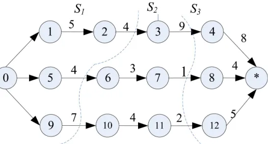
by

feasible solution for JSP. Figure 1 illustrates a disjunctive graph for a job shop scheduling problem with 3 jobs and 3 machines.

Figure 1. An illustration of a disjunctive graph for a job shop scheduling problem with 3 jobs and 3 machines

The job shop problem can be formulated as follows:

(1)

(2)

(3)

(4)

where, C denotes the set of the last operation of each job;

P

j and

t

j are the processing time

and starting time of operation j respectively;

w

j and

d

j are the weight and due-date of the job

to which operation j belongs. Equation (1) is the scheduling objective of the total weighted tardiness; Equation (2) describes the operation precedence constraints for the operations of each job; Equation (3) ensures that no job can start in the past; Equation (4) describes the machine capacity constraints to make sure each machine can process only one job at a time.

3. The algorithm

focuses on two aspects: (1) The large-scale JSP is decomposed into a series of sub-problems to reduce the computing scale. And then each sub-problem corresponds to a small-scale JSP. The solution of the large-scale JSP can be obtained by iteratively solving the sub-problems. (2) According to the principle “Bottleneck leads the performance of the whole manufacturing system” in TOC (Watson, Blackstone & Gardiner, 2007; Costas, Ponte, Fuente, Pino & Puche, 2014), the bottleneck machines should get more attention than the non-bottleneck machines. Therefore in the solving process of the sub-problems, the bottleneck operations are scheduled by genetic algorithm for high solution quality, and the non-bottleneck operations are scheduled by dispatching rules for the improvement of the solving efficiency.

3.1. The definition of the sub-problem

DH-MB decomposes the operations of the large-scale JSP to construct sub-problems one by one according to the process routes of the jobs. In a sub-problem of the large-scale JSP, a set o f

n

jobs are to be processed on a set of

m

machines. Each job

J

i

(

i

= 1 …

n

)

contains

m

i

(

m

i

≤

m

)

operations which have the operation precedence constraints and consist with the

assumptions of the original JSP. The model of the sub-problem can be formulated as follows:

(5)

(6)

(7)

(8)

where,

C

sub is the set of the last operations of each job in the sub-problem;

A

sub denotes the

operation precedence constraints for the operations in the sub-problem;

S

i is the arriving time

of

J

i;

f

i is the finish time of

J

i in the previous scheduled sub-problem; is the

set of the operations in the sub-problem.

3.2. The sub-problem construction

In order to overcome the flaw in the sub-problem construction described above, DH-MB constructs the sub-problems by separating some operations along the processing route of each job. The decomposing process follows the principle of “Uniform Distribution Load” to make sure that the load of each job distributes uniformly in each sub-problem. Then each sub-problem contains some operations of each job to avoid the phenomenon that some jobs finish in advance and some jobs delay severely. The decomposing process is as follows:

Step 1: Input the number of sub-problems (P), and then the average load of each job in each

sub-problem can be determined by .

Step 2: Initialize the sub-problem

S

k,

k

= 0. Set

S

k = , and the load of each job in

S

k is

l

i = 0.

Step 3: Start decomposing the operations of the jobs. For each job, take the first un-separated

operation

φ

into the constructing sub-problem along the processing route. Set

S

k =

S

k

∪φ

and

l

i=

l

i

+ p

iφ.

Step 4: If

l

i

<

L

i and 

<

m

, then return to Step 3; else go to Step 5.

Step 5: Fix c. If all the operations of each job are decomposed, then stop; else make

k

=

k

+ 1,

return to Step 3.

Figure 2 illustrates the decomposition scheme for a JSP with 3 jobs and 4 machines. In the JSP, the number of sub-problems is 3, the total load of each job is (26, 12, 18), and then the average load of each job in one sub-problem is (9, 4, 6). According to the sub-problem

construction method above, the number of operations of each job in

S

1 is (2, 1, 1), and

S

2 is

(1, 2, 2), and

S

3 is (1, 1, 1).

Theorem: By constructing the sub-problems sequentially, the solution of each sub-problem doesn't conflict with the processing route of each job in the original large-scale JSP, and the solution of the original problem can be easily obtained by solving the sub-problems.

Prove: (1) According to the definition of problem, the order of operations in each sub-problem consists with the operation precedence constraints of the jobs. Therefore the solution of each sub-problem cannot conflict with the processing route of each job in the original large-scale JSP. (2) If the original JSP is decomposed into p sub-problems , the sub-problems

have different priority levels which can be noted as

S

1 ≺

S

2 ≺ ... ≺

S

p (

X

≺

Y

represents that

the operations in

X

have higher scheduling priority than the operations in

Y

). For any two

operations

O

i and

O

j, if

(

O

i,

O

j

)



A

and

O

i 

S

1,

O

j 

S

2，then

S

1 ≺

S

2 (Zhang & Wu, 2010). Therefore the operations in adjacent sub-problems also satisfy the operation precedence constraints of the jobs.

From (1) (2), we can know that this decomposition method doesn't destroy the operation precedence constraints of each job. And then the solution of the original problem can be obtained by solving the sub-problems.

3.3. The sub-problem solving

3.3.1. Multi-bottleneck detection based on critical path method

By decomposing the original problem, the number of operations in each sub-problem is not very large, so it can be solved by genetic algorithm (GA) which is effective for small-scale JSPs. However in order to improve the solving efficiency, DH-MB adopts different scheduling strategies for different types of operations. The operations are divided into two types: the bottleneck operations which are processed on the multi-bottleneck machines and the non-bottleneck operations which are processed on the non-non-bottleneck machines. And a detection method based on critical path is proposed for the multi-bottleneck machines. The method is as follows：

which more critical operations will be processed may have the greater possibility to be a bottleneck machine.

For a job shop scheduling problem, different schedules may have different critical paths. Therefore for many different schedules, the machine statistically with larger average value and smaller fluctuation of critical operation number may have greater possibility to be a bottleneck. In this paper, a few different frequently used dispatching rules are adopted and randomly combined to generate many different feasible schedules (The dispatching rules are FCFS, FCLS, SPT, LPT, LWKR, MWKR, FOPNR, GOPNR, NINQ, WINQ, EDD, ODD, SL and OSL (Haupt, 1989)). For each schedule, the critical operation number of each machine is taken as the sample value. Then the multi-bottleneck machines can be detected by the bottleneck detection model which is as follows:

(9)

(10)

(11)

Where,

v

i is the bottleneck possibility of machine

i

;

N

is the sample number (It is 500 in the

simulation of Section 4);

μ

i is the average value of the critical operation number of machine

i

;

b

ij is the critical operation number of machine

i

for the sample

j

; is the variance value of the

critical operation number of machine

i

, and reflects the fluctuation of the critical operation

number of machine

i

; the constant

ρ

denotes the correction factor which avoids

v

i too small to

compare (It is 100 in the simulation of Section 4).

In the bottleneck detection model, both the average value and the fluctuation of the critical

operation number are taken into account. The machine with larger

v

i represents that the

machine has larger average value and smaller fluctuation of the critical operation number. Correspondingly the machine has greater possibility to be a bottleneck machine. So according to the bottleneck detection model and the sample value, by sorting the

v

i of each machine

decreasingly, the higher the machine ranks, the greater possibility the machine will have to be a bottleneck machine. In the simulation of Section 4, we choose 30% of the machines as the

3.3.2. The solving process for the sub-problem

DH-MB adopts different scheduling strategies for the bottleneck machines and non-bottleneck machines. For the bottleneck machines which have great impact on the performance of the system, GA is adopted for an optimal and effective schedule. For the non-bottleneck machines, a dispatching rule which selects the job with the earliest modified due-date (MOD) is adopted to get a schedule efficiently.

If the bottleneck machines and non-bottleneck machines are scheduled independently, there may be conflictions between the schedules of the bottleneck machines and non-bottleneck machines. In DH-MB, the scheduling of the non-bottleneck machines is integrated in the decoding process of the scheduling of the bottleneck machines, thus the bottleneck operations and non-bottleneck operations can be scheduled parallelly to avoid the coordination between the schedules of the bottleneck machines and non-bottleneck machines, and the efficient of DH-MB can be improved obviously.

The GA in DH-MB uses operation-based coding method which can easily decode the chromosome into an active schedule. The LOX operator and SWAP operator (Wang, 2003) are adopted to generate new chromosomes for maintaining the population diversity. In the decoding phrase, the operations in the previous scheduled sub-problem already have fixed start and finish time, so the chromosome is decoded based on the schedule result of the previous scheduled sub-problem. The decoding process is as follows:

Let

PS

denote the set of the operations which are already scheduled;

S

denotes the set of

operations to be scheduled currently;

σ

i denotes the earliest start time of operations

i

in

S

,

ϕ

i

denotes the earliest predicted completion time of operations

i

in

S

;

C

denotes the set of conflicting operations which satisfy the scheduling condition.

Step 1: Let

PS

= ,

S

be the set of operations which are the first unscheduled operations on

the processing route of each job.

Step 2: Get

ϕ

* ₌

min

iS

{

ϕ

i

}

and

m

* on which the corresponding operation of

ϕ

* will be

processed. If there is more than one machine, choose one machine randomly.

Step 3: Establish the conflicting operation set

C

with the operations which are processed on

m

* _and

σ

i <

ϕ

*

(

i  S

)

.

Step 4: Select one operation s to schedule.

I f

m

* _{is a bottleneck machine, then s is the first unscheduled operation in the decoding}

arg min

iC , =

max

iC

(

ϕ

i, di

)

; if there are more than one operation, select one operation

randomly.

Step 5: Compute and fix the start time and finish time for the operation

s

.

Step 6: Let

PS

=

PS

∪

s

. Update

S

. If

S

= , then the decoding process stops; Otherwise go to

step 2.

Since the operations in the current scheduling sub-problem is partial operations of the original JSP, the optimal solution in the sub-problem may not have the same optimal performance for the original JSP. So in order to improve the global optimality of the DH-MB, we propose a strategy that is evaluating the chromosome's fitness in the sub-problem by predicting the global scheduling objective (EF-PGSO) of the original JSP. Specifically, in the decoding process of each chromosome in the sub-problem, we try to obtain a complete schedule by scheduling the remaining unscheduled operations which are not in the current scheduling sub-problem using the dispatching rule of MOD, and the objective value of the complete schedule is used as the evaluation value of the chromosome in the sub-problem.

3.4. The connection of the adjacent sub-problem

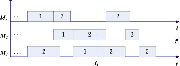
In DH-MB, the solving process of each sub-problem corresponds to a time window in the whole scheduling time domain. At the end of each time window, not all the jobs can complete at the same time. Figure 3 shows a schedule of one sub-problem

S

k (

k

is not the last serial number of

the sub-problems). At time

t

1, all the decomposed operations of job J1 in

S

k are scheduled, and

there are still unscheduled decomposed operations of job

J

2 and

J

3 left. Therefore after time

t

1,

j o b

J

2 and job

J

3 are scheduled without considering the resource utilization of the rest

undecomposed operations of job

J

1 in

S

k+1. If the sub-problem

S

k+1 is directly constructed following on the scheduling result of

S

k without any process, then the earliest start time of the

first unscheduled operation of job

J

1 in

S

k+1 will be delayed because job

J

2 and job

J

3 have used the resource in advance in

S

k. So the global optimal performance of DH-MB will be weakened

Figure 3. An illustration of the schedule of one sub-problem Sk

In order to avoid the one-sidedness in the solving process of the sub-problems, we propose a strategy that divides partial operations in the previous scheduled sub-problem into the adjacent sub-problems for re-optimization (DPO-AS).

The re-optimization operations are:

(12)

Where,

σ

i is the starting time of operation i;

c

j is the completion time of job

J

j.

The strategy can strength the connection between the solutions of the sub-problems, and the construction of the next sub-problem is closely linked to the solution of the previous scheduled sub-problem. All the sub-problems are dynamically constructed in the solving process of the sub-problems. Therefore all the jobs can be scheduled with equal resource competition, and the global optimization of DH-MB can be improved.

3.5. The specific steps of DH-MB

Step 1: Initialization. Input the sub-problem number P, then the average load of each job in

each sub-problem is . Let

N

C _{=  denote the set of scheduled operations. Let}

N

NC ₌

N

_{denote the set of unscheduled operations. Set the serial number of the current}

sub-problem k=1, the current sub-sub-problem

S

k = , and the re-optimization operations set

N

J = .

Step 2: Multi-bottleneck detection. According to the multi-bottleneck detection method in section 3.3.1, determine the bottleneck machines in the large-scale JSP.

Step 3: Construct

S

k according to the sub-problem construction method in Section 3.2 and the

3a: Let

l

i = 0,

i

= 1 ...

n

denote the load of job

i

. Add the re-optimization operations in the

previous scheduled sub-problem into

S

k, and calculate the load of job

i

, where

is the re-optimization operations of job i.

3b: According to the processing route of job

i

, take the first operation

φ

from the set of

unscheduled operations. Let

S

k = Sk

∪

φ

, then

l

i=

l

i +

p

iφ.

3c: if

l

i <

L

i and

φ <

m

, go to 3b; otherwise go to Step4.

Step 4: Solve the sub-problem

S

k according to scheduling method in Section 3.3.2.

Step 5: Determine the re-optimization operations

N

J _{according to Section 3.4 and fix the}

schedule of the operations in

S

k except

N

J. Let

N

C = NC

∪(

S

k\

N

J

)

,

N

NC = NNC

\

(

S

k\

N

J

)

.

Step 6:If

N

NC ₌

, then the algorithm stops; Otherwise let k=k+1, and go to step 3.

4. Simulation results and analysis

4.1. The generation of the testing instances and DH-MB parameters

In order to analyze the performance of DH-MB, 12 JSP instances are generated for simulation. The instances contain 1 small-scale instance (S1), 2 medium-scale instances (M1 and M2) and 9 large-scale instances (L1~L9). In each instance, the processing route of each job is a random permutation of m machines, the (integral) processing time of each operation follows a uniform distribution U [1, 100], and the due-date of each job is set according to reference (Feng, Leung & Tang, 2005):

(13)

Where r=1.5.

In DH-MB, the parameters of GA are:

• The mutation probability

p

m= 0.1;

• The population size

popsize

= 50;

• The number of exiting iterations

GN_exit

= 20; (If the performance of the optimal solution is not improved in 20 iterations, then the algorithm exits and exports the optimal solution.)

We compare DH-MB with the following frequently-used scheduling methods:

• Dispatching Rules (DR): three dispatching rules (EDD/MDD/SL) are selected and the optimal result of the three dispatching rules is taken as the final result;

• Standard Genetic Algorithm (SGA): the parameters of SGA are the same to DH-MB;

• Constraint Scheduling Algorithm (CSA) (Zuo, Gu & Xi, 2008).

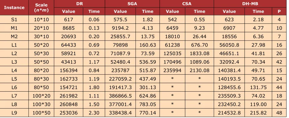
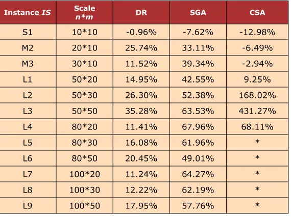
Considering the randomness of the GA, we use DH-MB and SGA to schedule each instance for 10 times, and the average of the objective values of the 10 schedules is selected as the final value, the average of the solving time in seconds of the 10 schedules is selected as the running time. Table 1 shows the final value and the running time of each instance using different scheduling methods. Table 2 shows the percentage of the value of DH-MB better than other methods which can be calculated as follows:

(14)

Where,

WT

(

X, IS

)

is the final value of instance

IS

calculated by method

X

.

From Table 1 and Table 2, we can see that the performance of DH-MB is slightly inferior to the other scheduling methods for the small-scale instance (S1). That is because DH-MB decomposes the original problem into a few sub-problems, and the schedules which is optimal for the sub-problems is not equal to be optimal for the original problem.

Instance (Scalen*m) DR SGA CSA DH-MB

Value Time Value Time Value Time Value Time P

S1 10*10 617 0.06 575.5 1.82 542 0.55 623 2.18 4

M1 20*10 8685 0.13 9194.2 4.13 6459 9.23 6907 4.77 10 M2 30*10 20693 0.20 25855.7 13.75 18010 26.44 18556 6.36 7 L1 50*20 64433 0.69 79898 160.63 61238 676.70 56050.8 27.98 16 L2 50*30 58921 0.72 71087.9 73.59 125035 1833.08 46651.1 41.81 26 L3 50*50 43413 1.17 52480.4 536.59 170496 1089.06 32092.4 70.34 42 L4 80*20 156394 0.84 235787 515.87 235994 2130.08 140381.4 49.71 15 L5 80*30 162733 1.19 227059.2 437.49 * * 140193.5 70.65 24 L6 80*50 154721 1.80 191417.3 301.13 * * 128455.6 131.75 44 L7 100*20 261982 1.11 386866.5 624.86 * * 235509.3 74.02 18 L8 100*30 260848 1.50 377001.4 783.05 * * 232450.2 119.00 24 L9 100*50 253036 2.30 338438.4 770.14 * * 214532.8 215.82 48

Instance IS Scale_n*m DR SGA CSA

S1 10*10 -0.96% -7.62% -12.98% M2 20*10 25.74% 33.11% -6.49% M3 30*10 11.52% 39.34% -2.94% L1 50*20 14.95% 42.55% 9.25% L2 50*30 26.30% 52.38% 168.02% L3 50*50 35.28% 63.53% 431.27% L4 80*20 11.41% 67.96% 68.11%

L5 80*30 16.08% 61.96% *

L6 80*50 20.45% 49.01% *

L7 100*20 11.24% 64.27% * L8 100*30 12.22% 62.19% * L9 100*50 17.95% 57.76% *

The note of * represents there is no feasible solution in 1 hour of computing.

Table 2. The percentage of the value of DH-MB better than other methods (δ)

However, with the scale of the instances increasing, the solution quality obtained by DH-MB is obviously better than DR and SGA, and the solving efficiency is also better than SGA. The reason can be analyzed as follows: For DR, the dispatching rules can get feasible schedules quickly, but cannot ensure the optimality of the schedules; For SGA, the increasing of the problem's scale will lead to the great expansion of the solving space, also the premature convergence and randomness are usually associated with SGA itself, so the possibility of obtaining the optimal solution will decrease. In addition, the time consumed by the chromosome decoding process in SGA increases greatly with the number of the operations increasing, therefore the solving efficiency of SGA is inferior to DH-MB.

4.2. The influence of the strategies of DH-MB for the performance

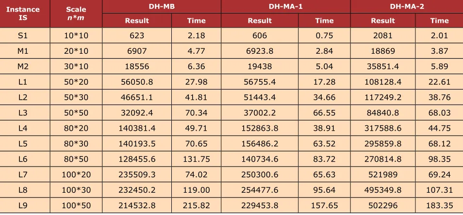
In order to analyze the influence of the strategies (EF-PGSO and DPO-AS), we compare the performance of DH-MB with and without the strategies to solve the JSP instances. We denote the DH-MB without the strategy of EF-PGSO as DH-MB-l, and the DH-MB without the strategy of DPO-AS as DH-MB-2. Table 3 shows the result of the calculation.

Instance

IS Scalen*m

DH-MB DH-MA-1 DH-MA-2

Result Time Result Time Result Time

S1 10*10 623 2.18 606 0.75 2081 2.01

M1 20*10 6907 4.77 6923.8 2.84 18869 3.87

M2 30*10 18556 6.36 19438 5.04 35851.4 5.89

L1 50*20 56050.8 27.98 56755.4 17.28 108128.4 22.61 L2 50*30 46651.1 41.81 51443.4 34.66 117249.2 38.76 L3 50*50 32092.4 70.34 37002.2 66.55 84840.8 68.03 L4 80*20 140381.4 49.71 152863.8 38.91 317588.6 44.75 L5 80*30 140193.5 70.65 156486.2 63.52 295859.8 68.12 L6 80*50 128455.6 131.75 140734.6 83.72 270814.8 98.35 L7 100*20 235509.3 74.02 250300.6 65.63 521989 69.24 L8 100*30 232450.2 119.00 254477.6 95.64 495349.8 107.31 L9 100*50 214532.8 215.82 229453.8 157.65 502296 183.35

Table 3. The influence of the strategies of DH-MB to the JSP instances

From Table 3, we can see that DH-MB-1 can save the solving time. The reason is that DH-MB-1 doesn't schedule the unscheduled operations which are not in the scheduling sub-problem. However, the solving process doesn't consider the global objective of the original JSP, and the optimal solution for the scheduling sub-problem may not be also optimal for the original JSP. So the solution of each sub-problem has local effect in DH-MB-1, and the solution quality of DH-MB-1 inferior to DH-MB. Therewith the strategies of EF-PGSO in DH-MB are beneficial to improve the solution quality of the original JSP.

5. Conclusion

In this paper, a decomposition heuristics based on multi-bottleneck machines is proposed for large-scale job shop scheduling problems. In the algorithm, the original problem is decomposed into a series of sub-problems to reduce the problem scale and solving complexity. The critical path method is adopted to detect the multi-bottleneck machines, and the characteristics of the bottleneck machine is used in the sub-problems' solving to improve the solving efficiency. The principle of “Uniform Distribution Load” and two strategies (DPO-AS and EF-PGSO) are proposed to improve the solution quality.

Simulation results show that, the performance of DH-MB is slightly inferior to other methods for the small-scale and medium-scale instances, but DH-MB has better performance for the large-scale instances. The algorithm can get satisfactory solutions within reasonable computational time for large-scale JSPs. In the end, we also analyze the influence of the two strategies (DPO-AS and EF-PGSO) to DH-MB, and the results verified their effectiveness on improving the solution quality.

Acknowledgment

The authors gratefully acknowledge the financial supports for this research from National Natural Science Foundation of China (Grant No. 51305024); Natural Science Project of Shaanxi Provincial Department of Education (2013JK1035), Natural Science Project of Xi’an Univ. of Arch. & Tech. (DB06035), and Natural Science Basic Research Program in Shaanxi Province (2012JM7017).

References

Bassett, M.H., Pekny, J.F., & Reklaitis, G.V. (1996). Decomposition techniques for the solution of large-scale scheduling problems. AIChE Journal, 42, 3373-3387.

http://dx.doi.org/10.1002/aic.690421209

Braune, R., Zäpfel, G. & Affenzeller, M. (2012). An exact approach for single machine subproblems in shifting bottleneck procedures for job shops with total weighted tardiness objective. European Journal of Operational Research, 218, 76-85.

http://dx.doi.org/10.1016/j.ejor.2011.10.020

Costas, J., Ponte, B., de la Fuente, D., Pino, R., & Puche, J. (2014). Applying Goldratt’s Theory of Constraints to reduce the Bullwhip Effect through agent-based modeling. Expert Systems with Applications, in press. http://dx.doi.org/10.1016/j.eswa.2014.10.022

Dalfard, V.M. & Mohammadi, G. (2012). Two meta-heuristic algorithms for solving multi-objective flexible job-shop scheduling with parallel machine and maintenance constraints.

Computers & Mathematics with Applications, 64, 2111-2117.

http://dx.doi.org/10.1016/j.camwa.2012.04.007

Feng, X., Leung, H., & Tang, L. (2005). An Effective Algorithm Based on GENET Neural Network Model for Job Shop Scheduling with Release Dates and Due Dates. Berlin/Heidelberg: Springer-Verlag. http://dx.doi.org/10.1007/11427391_124

Haoxun, C., Chengbin, C., & Proth, J.M. (1998). An improvement of the Lagrangean relaxation approach for job shop scheduling: a dynamic programming method. Robotics and Automation, IEEE Transactions on, 14, 786-795.

Haupt, R. (1989). A Survey of Priority Rule-Based Scheduling. OR Spektrum, 11, 3-16.

http://dx.doi.org/10.1007/BF01721162

Lin, R., & Liao, C.-J. (2012). A case study of batch scheduling for an assembly shop.

International Journal of Production Economics, 139, 473-483.

http://dx.doi.org/10.1016/j.ijpe.2012.05.002

Mönch, L., Schabacker, R., Pabst, D., & Fowler, J.W. (2007). Genetic algorithm-based subproblem solution procedures for a modified shifting bottleneck heuristic for complex job shops. European Journal of Operational Research, 177, 2100-2118.

http://dx.doi.org/10.1016/j.ejor.2005.12.020

Pinedo, M.L. (2008). Scheduling: Theory, Algorithms and Systems. New York: Prentice Hall.

Qingdaoerji, R., Wang, Y., & Wang, X. (2013). Inventory based two-objective job shop scheduling model and its hybrid genetic algorithm. Applied Soft Computing, 13, 1400-1406.

http://dx.doi.org/10.1016/j.asoc.2012.03.073

Scholz-Reiter, B., Hildebrandt, T., & Tan, Y. (2013). Effective and efficient scheduling of dynamic job shops—Combining the shifting bottleneck procedure with variable neighbourhood search. CIRP Annals - Manufacturing Technology. http://dx.doi.org/10.1016/j.cirp.2013.03.047

Sourirajan, K. & Uzsoy, R. (2007). Hybrid decomposition heuristics for solving large-scale scheduling problems in semiconductor wafer fabrication. Journal of Scheduling, 10, 41-65.

http://dx.doi.org/10.1007/s10951-006-0325-5

Watson, K.J., Blackstone, J.H., & Gardiner, S.C. (2007). The evolution of a management philosophy: The theory of constraints. Journal of Operations Management, 25, 387-402.

http://dx.doi.org/10.1016/j.jom.2006.04.004

Zhai, Y., Sun, S., Wang, J., & Niu, G. (2011). Job shop bottleneck detection based on orthogonal experiment. Computers & Industrial Engineering, 61, 872-880.

http://dx.doi.org/10.1016/j.cie.2011.05.021

Zhang, C.Y., & Li, P., Rao, Y., & Guan, Z. (2008). A very fast TS/SA algorithm for the job shop scheduling problem. Computers & Operations Research, 35, 282-294.

http://dx.doi.org/10.1016/j.cor.2006.02.024

Zhang, R. & Wu, C. (2010). A hybrid approach to large-scale job shop scheduling. Applied Intelligence, 32, 47-59. http://dx.doi.org/10.1007/s10489-008-0134-y

Zuo, Y., Gu, H., & Xi, Y. (2008). Study on constraint scheduling algorithm for job shop problems with multiple constraint machines. International Journal of Production Research, 46, 4785-4801. http://dx.doi.org/10.1080/00207540701324143

Journal of Industrial Engineering and Management, 2014 (www. jiem. org)

Article's contents are provided on a Attribution-Non Commercial 3. 0 Creative commons license. Readers are allowed to copy, distribute and communicate article's contents, provided the author's and Journal of Industrial Engineering and Management's names are included.