The equatorial E-region and its plasma instabilities: a tutorial

D. T. Farley

School of Electrical and Computer Engineering, Cornell University, Ithaca, NY, USA

Received: 7 October 2008 – Revised: 19 February 2009 – Accepted: 19 February 2009 – Published: 2 April 2009

Abstract. In this short tutorial we first briefly review the ba-sic phyba-sics of the E-region of the equatorial ionosphere, with emphasis on the strong electrojet current system that drives plasma instabilities and generates strong plasma waves that are easily detected by radars and rocket probes. We then dis-cuss the instabilities themselves, both the theory and some examples of the observational data. These instabilities have now been studied for about half a century (!), beginning with the IGY, particularly at the Jicamarca Radio Observatory in Peru. The linear fluid theory of the important processes is now well understood, but there are still questions about some kinetic effects, not to mention the considerable amount of work to be done before we have a full quantitative under-standing of the limiting nonlinear processes that determine the details of what we actually observe. As our observational techniques, especially the radar techniques, improve, we find some answers, but also more and more questions. One dif-ficulty with studying natural phenomena, such as these in-stabilities, is that we cannot perform active cause-and-effect experiments; we are limited to the inputs and responses that nature provides. The one hope here is the steadily growing capability of numerical plasma simulations. If we can accu-rately simulate the relevant plasma physics, we can control the inputs and measure the responses in great detail. Unfor-tunately, the problem is inherently three-dimensional, and we still need somewhat more computer power than is currently available, although we have come a long way.

Keywords. Ionosphere (Electric fields and currents; Equa-torial ionosphere; Ionospheric irregularities)

Correspondence to: D. T. Farley ([email protected])

1 Introduction

Plasma instabilities in the ionospheric E-region are driven by the currents that flow at E-region altitudes and by the electron density gradients there. We now know that these instabilities can be detected at times at any latitude, but they are most common, and strongest, at equatorial latitudes and in the au-roral zone, where they have been detected by radars for at least six decades. The instabilities generate plasma waves, with phase fronts highly aligned with the geomagnetic field; any waves that are not so aligned are rapidly destroyed by diffusive damping.

The currents that drive the instabilities flow perpendicu-lar to the geomagnetic field. Such currents are particuperpendicu-larly strong in the auroral zone and at the equator. The high lati-tude currents are often very strong because the electric fields, driven by the solar wind and magnetospheric dynamo, can be very strong: 50–100 mV/meter is not uncommon. At equa-torial latitudes, which are our concern here, the currents and electric fields are driven by tidal winds at low and middle latitudes and are weaker, but stronger than at mid latitudes.

The current flow patterns at low latitudes are determined both by the winds and by the conductivities, which are small at night because of the low electron densities, and vary strongly with altitude during the day. The strongest tidal winds in the E-region are driven by the 24-h “tide” asso-ciated with solar heating. To lowest order, the winds flow away from the subsolar point towards midnight. In the lower E-region the electrons are strongly magnetized (eνe) but

The upshot of all this is that the daytime solar quiet (Sq)

low latitude E-region currents flow approximately counter clockwise in the Northern Hemisphere and clockwise in the southern, with foci at roughly±30◦magnetic latitude at the equinoxes. The details of this pattern vary with season and longitude, the latter due to the fact that the magnetic equator deviates substantially from the geographic equator in some locations (especially South America). The equatorial elec-trojet currents are strong not because the equatorial zonal electric fields are strong (they are usually quite weak, on the order of 0.5 to 1 mV/m typically), but because the conductiv-ities are unusually high in the narrow latitude region where the geomagnetic field is very nearly horizontal. TheSq

cur-rent system has been studied for decades using ground based magnetometers. During strong magnetic disturbances driven by the magnetosphere and solar wind, the current pattern can become quite distorted, and sometimes it actually reverses (producing a counter electrojet). As we shall learn, such a reversal has interesting consequences for the plasma insta-bilities.

In the sections to follow we look first at some basic pho-tochemistry and related time constants, and next at the con-ductivity tensor and what happens near the magnetic equa-tor. Much of this material follows standard treatments in texts such as Rishbeth and Garriott (1969) and Kelley (1989). Then we move on to consider the basic features of the E-region plasma instabilities and some of the assumptions that are commonly made for the equatorial case. This tutorial is meant to be an introduction to the instabilities rather than a complete review of five decades of work. A very thorough discussion of most of the current state of the art has recently been given by Hysell et al. (2007).

2 Production and loss of ionization

The equation of continuity for the electron concentrationN is

∂N

∂t =q−`(N )−div(NV) (1)

whereq is the production rate,`(N )is the loss rate, and the last term is the transport term (V is the velocity). Transport is usually not important during the day in the E-region (but it may matter at night for long lived metallic ion layers). And for the zero order densities the time derivative is usually neg-ligible and the production and loss terms balance each other, producing photochemical equilibrium. The time derivative and transport terms do matter, however, when we consider plasma instabilities.

The production is due to photoionization by solar extreme ultraviolet (EUV) radiation that produces mostly molecular ions, plus some metallic atomic ions associated with meteor debris. The most important loss mechanism in the E-region is dissociative recombination, described by

XY++e→X∗+Y∗ (2)

where the asterisks indicate excited states, and with a rate coefficientαe∼10−13m3s−1, meaning that

∂N

∂t =αe[N][XY +_{] =}

αeN2 (3)

so for typical equatorial electron and ion daytime densities of the order of 1011m−3, the decay timeτ=[N−1∂N/∂t]−1 would be about 102s, which is very short compared to a day (but very long compared to the time scales λ/V of all but very long plasma waves). The transport term time constant will also be very long for the zero order profile since the am-bient electron density gradients are essentially vertical and the velocities are essentially horizontal.

At night, however, the situation is quite different. The molecular ion densities are one or two orders of magnitude smaller, so the dissociative recombination times are corre-spondingly longer, and sometimes metallic ions may domi-nate the density profile, in which case we must consider ra-diative recombination, namely

X++e→X∗→X+hν (4)

with now a much smaller rate coefficient of αe∼10−18m3s−1, corresponding to a time constant of

many days! So there is plenty of time for suitable winds and electric fields to generate thin layers with relatively high density. (The reason thatαe is so much smaller for Eq. (4)

than for Eq. (2) is that it is much harder to conserve both energy and momentum for Eq. (4).)

Attachment and detachment of electrons to and from neu-tral molecules can also destroy or create free electrons, but these processes are not important at the altitudes we are in-terested in.

3 Equatorial electrojet conductivities

The electrical conductivity in the ionosphere is highly anisotropic, which we describe with the tensor

σ =  

σp 0 σh

0 σ0 0

−σh 0 σp



 (5)

where the Cartesian coordinates point eastward, northward (parallel to B), and upward at the equator, and the parallel, Pedersen, and Hall conductivities are described by

σ0

N e2 =k0e+k0i,

σp

N e2 =kpe+kpi,

σh

N e2 =khe−khi(6)

where the mobilities are given by

mνk0=1, mνkp= ν2

ν2+2, mνkh= ν

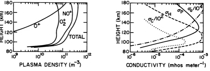
Fig. 1. Vertical profiles of daytime composition and plasma density (left) and conductivities (right) for average solar conditions (from Forbes and Lindzen, 1976.)

electrons, as appropriate. We also note that the electron term dominates the parallel and Hall conductivities, whereas the ions dominate the Pedersen conductivity. For example, for an eastward E, the electrons wouldE×Bdrift upward, cor-responding to a downward (negative) vertical current, while the ions would move slowly eastward. Some typical conduc-tivity profiles are shown in Fig. 1.

The daytime low and middle latitude horizontalSq

cur-rents are driven fundamentally by the poleward winds de-scribed in the Introduction interacting with the vertical com-ponent of the geomagnetic field. This vertical comcom-ponent is of course very small at low latitudes, so the wind driven currents flow mainly westward (eastward electron drift) at latitudes above 30 degrees or so. In the nighttime hemi-sphere the E-region densities are very low and so, to maintain ∇·J=0, a positive (negative) charge builds up at the dawn (dusk) terminator. This charge distribution drives the ward daytime equatorial return current. The associated east-ward electric field, as already mentioned, is comparatively weak, perhaps 0.5 mV/m. Why are the electrojet currents so strong?

This happens because vertical currents are strongly inhib-ited at the magnetic equator, since no vertical current flows parallel to the magnetic field (andσ0σh, σp). Below 90 km

or so the conductivity decreases rapidly because of the in-creasing collision frequencies, and above 140 km ions be-come magnetized and so the electrons and ionsE×B drift together and the Hall conductivity drops. As a crude approxi-mation, then, we can consider the electrojet layer, centered at about 103–105 km, to be bounded above and below by insu-lating regions. Polarization charges build up on these bound-aries to (almost) prevent vertical current flow in the layer. Then from Eq. (5) we find that

Jz = −σhEx+σpEz'0 H⇒ Ez' σh σp

Ex (8)

The Hall/Pedersen conductivity ratio reaches a maximum value of 15–20 in the vicinity of 103–105 km, and so the up-ward polarization field is an order of magnitude larger than the original driving zonal field. This field now drives an

east-Fig. 2. The slab geometry model of the equatorial electrojet (from Kelley, 1989).

ward Hall current (consisting mainly of a westward electron drift), and so the effective conductivity in terms of the origi-nal zoorigi-nal electric field is increased fromσpto what is known

as the Cowling conductivity

σCowling=

σ_h2 σp

+σp (9)

The slab model geometry is shown in Fig. 2.

If we are slightly off the magnetic equator, at a dip angle ofI, a little algebra shows that this last result would be

σxx =

σ_h2cos2I σ0sin2I +σpcos2I

+σp (10)

which reduces to the Cowling result forIp

σp/σ0, i.e., a

few degrees or less. So the equatorial electrojet is confined to a narrow band of latitude only a few hundred kilometers wide.

Farther off the equator the vertical current may not be zero because field aligned currents will flow in response to north-south asymmetries in the global wind system, in order to nearly equalize the potentials at opposite ends of the mag-netic field lines.

which will produce a westward electron drift velocityE/Bof about 400 m/s (B'0.25 gauss at the equator), which will ex-cite unstable, westward traveling plasma waves, as we shall see. The typical noontime electrojet current density reaches maximum values of the order of 10−5amps m−2and causes a typical midday increase in the equatorial (horizontal) geo-magnetic field of the order of 100 nT.

This slab model of the equatorial electrojet was essentially verified by the 1994 in-situ rocket measurements in Brazil (the Guar´a campaign) described by Pfaff et al. (1997). The vertical polarization field is difficult to measure since the rocket has to be oriented parallel to the magnetic field, but this was achieved in 1994, and the authors found a maximum value of the daytime vertical electric field near the altitude of 105 km to be about 9 mV/m, corresponding to a westward electron drift of about 360 m/s. Some details of the data did not fully agree with the simple model, but the key feature of the large induced vertical polarization field driving a large Hall current was fully confirmed.

At night this whole scenario reverses sign and the currents are westward. The nighttime currents are much weaker, how-ever, because the electron densities are so much smaller, and so they cannot be studied effectively by magnetometer net-works on the ground. The electric fields and the electron drift velocities, however, are comparable to the daytime val-ues, and so again can easily drive plasma instabilities.

The other important parameter for the instabilities is the electron density profile, which is smooth with an upward gradient until about 107 km or so during the day, but be-comes very jagged with sharper gradients and lower densities at night.

4 Electrojet plasma instability theory 4.1 Basic ideas

We begin with a quick summary of the well known linear fluid theory of the equatorial electrojet instabilities and then review the perhaps not quite so familiar assumptions that are usually made for the equatorial electrojet case (only; some of these assumptions are not valid at high latitudes). The plasma waves are electrostatic, longitudinal waves (wave vectors parallel to the wave electric field and velocity perturbations). The equations we need are the continuity equations already given in Eq. (1) for the ions and electrons, the equations of motion or momentum (for no neutral wind)

mNdV

dt =qN (−∇8+V ×B)− ∇P −mνNV (11) for the ions and electrons (8is the electrostatic potential,P is the particle pressure, andB is the (constant) geomagnetic field in the above), and Poisson’s equation

∇28= −(e/0)(Ni−Ne) (12)

For scale lengths much larger than the Debye length (λD∼3 mm in the electrojet region), Poisson’s equation

can be replaced with Ne≈Ni=N. We also, for now, set P=N KT, the isothermal case, withK being Boltzmann’s constant.

The next step is to linearize all the equations, with the per-turbations being sinusoidal traveling waves, i.e.,

N →N0+nexp[i(k·r−ωt )] (13)

with similar expansions for8 andV. Such “local” plane wave solutions are valid so long as the wavelengths of inter-est are small compared to the dimensions of the electrojet. We now eliminate the zero order terms, put the equations for the first order perturbations in matrix form, noting that ∂/∂t→−iωand∇→ik for the perturbations, i.e.

  

a11 · · ·an1

.. . . .. ... a1n· · ·ann

      b1 .. . bn  

=0 (14)

where the column vector consists of the unknown pertur-bations, and then we set the determinant of the coefficient matrix equal to zero to find the dispersion equation relating ω to the wave vector k. The last step is to set the (com-plex)ω=ωk+iγk and further assume that the magnitude of

the growth (or damping) rate|γk||ωk|.

All this leads finally to the “standard” local linear fluid theory (e.g., Fejer et al., 1975, and several earlier references) for the equatorial electrojet plasma waves in the frame of the ions (essentially the frame of the neutral wind), namely ωk=

k·Vd

1+ψ (15)

for the real part of the angular oscillation frequency and γk =

ψ (1+ψ )νi

( ω2_k |{z}

1

−k2C2_s | {z }

2

)+ νi i

ωkkwest

Lk2

| {z }

3

−2αN | {z }

4

(16)

for the growth rate (s−1), where

ψ (θ )=ψ0

k_⊥2 k2 +

2_ek_k2 ν2

ek2

! ≈ νeνi

ei

1+

2 e ν2 e θ2 ! (17)

andL=n0(dn0/dh)−1is the vertical gradient length (which

is assumed for a local theory to be large compared to wavelengths of interest),Cs is the isothermal (usually)

ion-acoustic velocity, Vdis the electron drift velocity relative to

the ions,αis the recombination rate, k=kplasmais the wave

vector (with a westward component kwest), and the aspect

angle θ is the complement of the angle between k and B, and so θ→0⇒k⊥B. The aspect angle effects are all con-tained in the last term in Eq. (17). For radar backscatter kplasma=2kradar.

Fig. 3. Electron density profiles and irregularity amplitudes over Thumba, India around noon and midnight. Note the effects of the density gradients (rom Prakash et al., 1972).

(3) the destabilizing or stabilizing effect of the electron den-sity gradient, and (4) stabilization by recombination, which is negligible except for very long wavelengths and the asso-ciated long time scales. Recombination is unimportant for the wavelengths of a few meters or less associated with radar echoes but usually limits very long, horizontally propagating waves to lengths no greater than a kilometer or two during the day. The waves can be significantly longer at night, when the recombination is substantially reduced, and then nonlocal effects (which we neglect here) may become important.

The crucial density gradient term is always positive (up-ward) during the day to altitudes of at least 105–107 km due to the photochemical equilibrium; at higher altitudes the day-time gradient becomes very small or even slightly negative (Pfaff et al., 1987a), as we shall see later. In the evening, as the layer decays, however, the positive gradient will extend higher, and at night, once the electron densities have dropped by one or two orders of magnitude, the density profile is con-trolled by dynamics, not photochemistry, and becomes very jagged, with upward and downward gradients (positive and negative values ofL) throughout the region.

So the gradient term (3) is always destabilizing throughout most of the electrojet region during the day for the normal eastward current flow (westward electron drift and westward traveling waves; i.e., positive values ofLfor a positivekwest).

For weak electric fields (drift velocitiesVdmuch smaller than Cs but not zero, so that ωk has the proper sign), we can

ignore term (1) as well as (4) in Eq. (16). Then, for long enough wavelengths (but not so long that neglected nonlo-cal effects become important), term (3) will always be larger than term (2) and the waves will grow. If the normal dynamo electric field should reverse during the day, as it sometimes does (counter electrojet), the unstable waves completely dis-appear unless the reversed drift is very large (which is rare). Excellent examples of both of these counter electrojet cases are given in Woodman and Chau (2002).

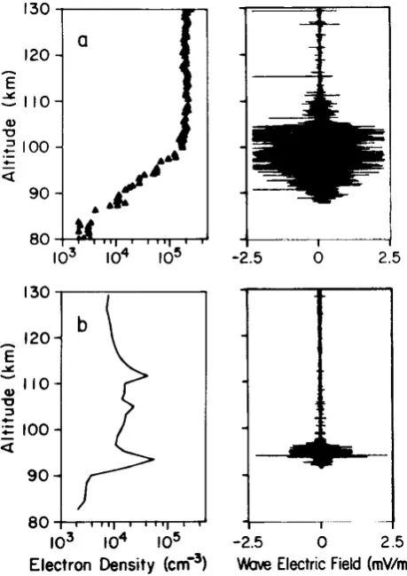
Fig. 4. Daytime (Peru, 1975; panel a) and nighttime (Kwajalein, 1978; panel b) rocket observations of density profiles and wave electric fields (from Pfaff et al., 1982).

At night, except near the time of the daily wind-driven dynamo electric field reversals, long wavelengths should al-ways be unstable; there will be regions of instability for ei-ther eastward or westwardVd.

Fig. 5. Rocket observations of density gradients and wave activ-ity. The waves change character where the profile flattens out (from Pfaff et al., 1987a).

Fig. 6. Daytime (10:34 LT on 12 March 1983) rocket observations of horizontal electric fields over Peru due to large scale waves. Note that the magnitudes are comparable to typical strong vertical

polar-ization fields and are much larger than the eastwardSqfield (from

Pfaff et al., 1987a).

Some additional interesting rocket data are shown in Figs. 5, 6 and 7. The first figure shows a daytime density profile over Peru that flattens out at about 105 or 106 km.

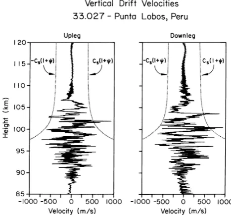
Fig. 7. Comparing the rocket data of the previous figure to the ion-acoustic threshold (from Pfaff et al., 1987b).

Below that height there are strong long wavelength waves. Above that height there is still some strong wave activity for a couple of kilometers, but these waves were short and were traveling mostly horizontally. In Fig. 6 we see that the hor-izontal wave electric fields can exceed 10 mV/m. These ob-servations, taken during the Condor campaign of 1983, are still the only in-situ observations taken during “two-stream” (see next paragraph) conditions. The very strong zonal per-turbation fields, comparable to the vertical polarization field and at least an order of magnitude larger than the zero order mean zonal field, show that the electrojet is not at all a nice laminar electron flow. Rather it is usually a highly turbulent flow whose mean velocity is (nearly but not quite) horizontal. Figure 7 shows the same wave data, but plotted differently to show roughly how it compares to the “two-stream” threshold velocity.

In the literature authors refer to (a) the “ion-acoustic” or “FB” or “two-stream” instability when term (1) in Eq. (16) exceeds term (2) and both are much greater than term (3), and to (b) the “gradient-drift” instability when (1) is small and (3) is positive and exceeds (2). In fact, of course, there is re-ally only one dispersion relation and one instability, but with two driving terms and two limiting cases, which depend on the plasma wavelength in quite different ways; the gradient-drift term dominates for long wavelengths. Case (a) pro-duces radar echoes known as “type 1” for historical reasons. These echoes are strong and have a Doppler spectrum that is sharply peaked at a phase velocity comparable to or some-what greater than the ion-acoustic velocityCs, usually at all

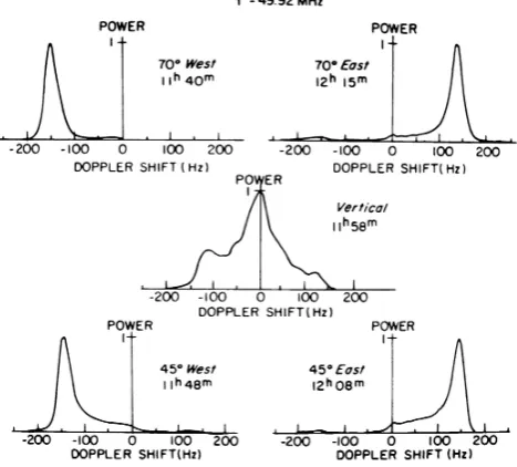
Fig. 8. Early Doppler spectra observations at Jicamarca at vari-ous zenith angles during a strong electrojet showing both type 1 and type 2 echoes. Note that the position of the echo peaks for the oblique echoes is nearly independent of zenith angle (from Cohen and Bowles, 1967).

corresponds to radar echoes known as “type 2”. These are weaker and have a broader Doppler spectrum with a peak in the vicinity ofω=kplasma·Vd. Figures 8 and 9 show

exam-ples from the Jicamarca Observatory in Peru in the 1960s of these two kinds of radar echoes.

Figure 8 shows type 1 echoes from overhead and from two substantially different oblique angles (both east and west), and both with almost the same Doppler shift, whereas Fig. 9 shows broader spectra with peaks whose position varies with the sine of the zenith angle, in general agreement with Eq. (15). The type 1 echoes, on the other hand, have their peak Doppler shift close to the value at the threshold of growth determined by the first two terms in Eq. (16). This last equation does not include kinetic effects, which can be significant. The effect of these is that the ion-acoustic veloc-ityCs increases somewhat with decreasing wavelength. This

dependence was nicely illustrated in an early paper (Bals-ley and Far(Bals-ley, 1971) that compared simultaneous radar ob-servations at radar frequencies of 16, 50, and 146 MHz. A sample of that data is shown in Fig. 10. Note the systematic changes in the type 1 peaks. No type 2 echoes were observed at 146 MHz, but the type 2 phase velocity spectra at 16 and 50 MHz (not shown here) matched exactly.

To summarize, then, the gradient term makes the electro-jet region unstable to longitudinal plasma waves most of the time in the electrojet region, but putting reasonable values of the ionospheric parameters into the growth rate expres-sion reveals that the unstable wavelengths will never be short

Fig. 9. Simultaneous type 2 echo Doppler spectra at 50 MHz at different zenith angles. The dashed lines show the means, which fit a sine dependence on the zenith angle for a 250 m/s velocity (from Balsley, 1969).

Fig. 10. Comparisons of type 1 spectra (mixed with some type 2 at 16 MHz on 16 May). The first and last observation of each group were made at the same frequency. Note the systematic shift in phase velocity with radar frequency. Type 2 echoes were not seen at 146 MHz (from Balsley and Farley, 1971).

0 0.2 0.4 0.6 0.8 1

105.3

Normalized Spectra

105.75 106.2 106.65 107.1 107.55 108 108.45 108.9 109.35 109.8 110.25 18:09:07 March 21, 2001

−500 0 5000 0.1 0.2 0.3 0.4 0.5

θ rms

[Degrees]

−500 0 500 −500 0 500 −500 0 500 −500 0 500 −500 0 500 Doppler Velocity [m/s]

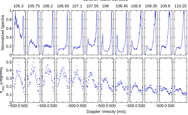
Fig. 11. Type 1 echoes from 105–110 km above Jicamarca in 2001. Note the simultaneous presence of both positive and negative peaks at times in the power spectra in the top row. The bottom row shows aspect angle data discussed below (from Lu et al., 2008).

that we see strong radar echoes even with a vertically di-rected radar. It is important to realize that the Bragg scatter-ing condition is a vector relationship that tells us that radar back-scattering from a sinusoidal plasma wave occurs only if kplasma wave=2kradar. For the large Jicamarca 50 MHz radar

this means that 3-m wavelength plasma waves propagating vertically are somehow excited (often strongly) by the hor-izontal electron flow. How can this happen when k·Vd is

apparently zero? In other words, how does the horizontal electron flow of the electrojet current couple energy into ver-tically propagating plasma waves with short wavelengths? These and related questions have led to a series of assump-tions that have been made explicitly or tacitly in the equato-rial literature for many years.

4.2 Common assumptions for the equatorial geometry 1. First of all, there is overwhelming radar and rocket ev-idence from Jicamarca and elsewhere that the “local back-ground” electric field is not just the dynamo field plus the larger vertical polarization field that arises to maintain a di-vergence free current flow even though the vertical conduc-tivity above and below the electrojet is nearly zero. The (al-most) ever present large scale wave fields strongly affect the background (the drift velocity term in Eq. 15), and so one cannot (as is sometimes implicitly done) automatically as-sume that there is a substantial “flow angle” between the directions of kradar and Vd, especially for the type 1 radar

echoes. As an extreme example of this flow angle problem,

consider the fact that, using the vertically pointing Jicamarca radar, we often observe (see Fig. 11 for example) daytime type 1 echoes with both positive and negative Doppler shifts at the same time and the same altitude!

This apparent paradox is explained by interferometry and imaging data (e.g., Farley et al., 1981; Hysell et al., 2007, and several earlier references therein) that show that the up-and down-traveling waves come from different portions of the (fairly small, usually) scattering volume, when the length of the dominant large-scale waves is smaller than the zonal dimension of the scattering volume (as it is during the day, but not at night). In other words, roughly horizontal elec-tric fields associated with the large-scale (kilometers) waves are as strong as or perhaps even somewhat stronger than the mean vertical electric fields, and so there will be large “local” background drift velocities more or less parallel to the radar k-vector for a wide range of zenith angles (including zero). Figure 12 shows a cartoon of the basic idea. Within a typi-cal radar scattering volume there can be a wide assortment of local drift velocities Vd.

observed dependence of the measured mean Doppler shift on the sine of the zenith angle, as we saw in Fig. 9. The drift velocity to be used in Eq. (15) is then the mean, not the very local velocities sketched in Fig. 12. This turbulent cascade also affects the aspect angles, as discussed in the next section. 3. When the dynamo field is strong enough, we see type 1 radar echoes with narrow frequency spectra that have Doppler shifts corresponding to velocities comparable to the ion-acoustic velocity (see Fig. 11). Furthermore, and perhaps somewhat surprisingly, to first order this observed Doppler shift does not depend on the radar zenith angle (see Fig. 8), in contrast to the type 2 echo case. (An exception to this be-havior is the example of type 1 echoes at Jicamarca during a very strong counter electrojet, described by Woodman and Chau, 2002).

The more or less generally accepted hypotheses for the normal electrojet behavior are that (1) the type 1 echoes are from plasma waves that are directly excited (γk>0) with a

wave vector of 2kradarby the highly turbulent drift velocities

and electric fields associated with the large scale (∼hundreds of meters or longer) waves, (2) the first two terms in Eq. (16) dominate the growth rate, and (3) in the nonlinear limit in which the mean growth rate goes to zero, the unspecified NL processes somehow conspire to force these two terms to cancel each other out. Hence the phase velocity is always approximatelyCs and not the value given in Eq. (15) if we

take Vd to be the more or less horizontal mean. Also, the

threshold phase velocity is probably not exactly the isother-mal value ofCs, either because of neglected thermal effects

and/or because of nonlinear processes. The question of the effect of thermal processes onCshas been discussed in

con-siderable detail in several recent papers, especially by Kis-sack et al. (2008a,b).

These thermal processes and the exact values of the type 1 velocity are not the focus of our concern here, however. In fact, we do not yet know if the dominant nonlinear lim-iting mechanism is two-dimensional (aspect angle effects are unimportant) or three-dimensional (coupling to damped waves propagating at off-perpendicular angles is the primary loss mechanism). There is a considerable literature covering analytical and numerical studies of 2-D mode coupling; see for example St.-Maurice and Hamza (2001), Otani and Op-penheim (2006), OpOp-penheim et al. (2008a), and earlier refer-ences therein. Unfortunately numerical simulations are still

Fig. 12. A sketch of the irregular electron velocity field in the

elec-trojet. Large scale instabilities produceE×Bvelocity perturbations

comparable to the mean values. The “local” velocities then drive small scale ion-acoustic instabilities, even in the vertical direction (from Farley and Balsley, 1973).

not yet able to deal well with both the coupling to small as-pect angles and the 2-D processes simultaneously with suffi-cient resolution.

In the high latitude (auroral) E region much of the physics is the same, but there are some major differences: (1) the driving electric fields are often much stronger at high lati-tudes, (2) the magnetic field is nearly vertical, so the impor-tant density gradients for the instability are horizontal, and (3) there are gradients in density, electron and ion tempera-tures, and collision frequencies parallel to the magnetic field that may affect the aspect sensitivity (the size ofθrms; see

Eq. 17). Furthermore, the different radar geometry makes it much harder to measure these aspect angles accurately with interferometry at high latitudes.

4.3 Magnetic aspect angles

An important parameter of the unstable electrojet plasma waves is the aspect angleθin Eq. (17), which is the angle by which the plasma wave vector deviates from perpendicular to the magnetic field. This parameter is important because even a small component of k parallel to B increases wave damp-ing and might cause electron heatdamp-ing, as is observed at high latitudes. Space limitations prevent going into this topic in detail here, but at least a few remarks are in order.

Using radar interferometry techniques with antennas spaced along a magnetic north-south line, it is possible to measureθ, or more particularlyθrms, the rms deviation ofθ

x

k₁ k₁

k₁ k₂

k₂

k₂

k₃ k3 k3

(a) (b) (c)

B

x y

Fig. 13. Possible 3-wave coupling interactions. In (a) two long un-stable waves drive a shorter wave, in (b) two short waves traveling roughly horizontally drive a longer (damped) wave traveling verti-cally, and in (c) a single long unstable horizontal wave drives two damped shorter waves traveling nearly vertically.

daytime “150 km” echoes. Some of the observations can be explained, qualitatively at least, by nonlinear mode coupling arguments of the sort described in the next section. One sam-ple of the recent observations is given in Fig. 10. The bottom panels of that figure show angles as small as 0.1◦ correspond-ing to the type 1 spectral peaks, but with values of the order of 0.4◦_{for small Doppler shifts at some altitudes.}

4.4 Nonlinear mode coupling

The data already presented make a strong case for the impor-tance of nonlinear mode coupling. It is easily shown that, no matter what the nonlinear process is, if two waves combine to form a third wave, they must obey the following rule: if waves (k1, ω1) and (k2, ω2) combine to form wave (k3, ω3)

then

k3=k1+k2 ω3=ω1+ω2 (18)

Note that the first equation above is a vector addition but the second is not. One or two of the waves must be growing and feeding energy to the remaining wave(s). This process is illustrated in the vector diagrams of Fig. 13.

Cases (a) and (c) in the figure represent a cascade from long wavelengths to short, the sort of process thought to be responsible for type 2 echoes. Case (b) is likely to be respon-sible for echoes that are sometimes seen by vertically point-ing radars in regions where there are no large scale waves (no density gradients) but strong electric fields; see Fig. 5, for ex-ample, above 105 km. This mode coupling has implications for the echo aspect angles also, as mentioned above. Cou-pling energy from long waves to short (e.g., case a) tends to reduce the aspect angle, whereas coupling from short waves to long (e.g., case b) tends to increase it (Kudeki and Farley, 1989; Lu et al., 2008).

4.5 Kinetic theory calculations

Several papers (e.g., Ossakow et al., 1975; Schlegel, 1983; St.-Maurice and Schlegel, 1983) have discussed linear ki-netic theory for the auroral zone E-region case, especially

when the electrojet is very strongly driven, withE×B drift velocities considerably larger than the ion-acoustic velocity. In this situation the linear growth rate, ignoring all gradi-ents, maximizes for slightly off perpendicular wave vectors. As an example, the calculations of Fig. 5a of St.-Maurice and Schlegel (1983) assumed a drift velocity of 1 km/s and a wavelength of 1 m. For ionospheric parameters appropriate to 105 km in the auroral zone, and with electron-to-ion tem-perature ratios somewhat larger than unity, they found a mild (double) maximum in the growth rate for angles between k and B of 90◦±0.4◦, which would mean a value ofθrmsof

per-haps 0.5◦or so, which is much larger than the values we see for type 1 echoes at the equator. The phase velocity of these primary waves was about 650 m/s, i.e., less than the drift ve-locity but more than the ion-acoustic veve-locity. The same pa-per made the (very) arbitrary assumption that the wave in-tensity (proportional to radar echo power) was proportional to the linear growth rate, leading to a Doppler spectrum that is not sharply peaked (their Fig. 1a). The upshot is that the linear kinetic theories so far proposed for the auroral zone predict neither the observed equatorial Doppler power spec-tra nor theθrmsvalues.

More recently Kissack et al. (2008a) and Kissack et al. (2008b) have written papers discussing in great detail ther-mal effects and their relation to aspect angles and flow an-gles. The problem with this is that it is dangerous to assume large flow angles, in particular, since, as we have seen, large scale velocities and electric fields are likely to be quite tur-bulent, at least at the equator, and radars will always respond most strongly to the regions where the flow angle is small. But large scale waves may not be so important in the auro-ral zone, since there the density gradients perpendicular to B that are important are horizontal, not vertical.

4.6 Numerical simulations and growth saturation

tions are our main hope of finding out what really matters. Of course trying to do sufficiently detailed (i.e., realistic) sim-ulations in three dimensions requires enormous computing power, but some exciting work has already been done (Op-penheim et al., 2008b).

5 Some final questions

This is far from a complete review of the subject, but it should provide some background for people relatively new to the field and perhaps a little food for thought for those of us working actively on electrojet instabilities. Some questions to think about include:

1. How important are flow angle and related thermal ef-fects at the equator? How much do they (or don’t they) affect the wave phase velocities and the aspect angles? How relevant to the equatorial case is the work done for the auroral zone? The measured aspect anglesθrms at

the equator are very small, in contrast (perhaps?) to the auroral zone. In any case, it seems clear that it is a se-rious mistake to assume that the electron flow is even remotely laminar over a significant range of space and time (e.g., the radar scattering volume and integration time), although this can happen occasionally during a daytime counter electrojet.

2. Is the dominant nonlinear process that limits wave growth primarily 2-D or 3-D? Will Moore’s law con-cerning computer power growth continue to hold long enough to give us the computer power to do really real-istic 3-D computer simulations? By “realreal-istic” I mean a simulation from which you can calculate the proper-ties of scattered radar pulses and in-situ fields and show that these agree with actual radar and rocket observa-tions. Once you can really do that, the computer can tell you what the dominant nonlinear processes are. For the equator, at least, the simulations should not be driven too hard, insofar as that is practical.

3. How different are the auroral and equatorial zones? Is the physics essentially the same, except for the fact that the auroral zone electric fields are often much stronger? Or is it important that in the auroral zone there are gra-dients parallel to the magnetic field in electron density,

cause of energy losses associated with the generation of strong plasma waves. Can simulations perhaps quan-titatively explain this also? Is there other confirming evidence? Is this something that global models need to worry about?

Acknowledgements. This work was supported by the Atmospheric Sciences Division of the National Science Foundation through Co-operative Agreement ATM-0432565 with Cornell University. This Agreement also supports the operations of the Jicamarca Radio Ob-servatory. I also thank Mike Kelley and Wesley Swartz for help in preparing this tutorial.

Topical Editor K. Kauristie thanks M. Uspensky and another anonymous referee for their help in evaluating this paper.

References

Balsley, B. B.: Some characteristics of non-two-stream irregulari-ties in the equatorial electrojet, J. Geophys. Res., 74, 2333–2347, 1969.

Balsley, B. B. and Farley, D. T.: Radar studies of the equatorial electrojet at three frequencies, J. Geophys. Res., 76, 8341–8351, 1971.

Cohen, R. and Bowles, K. L.: Secondary irregularities in the equa-torial electrojet, J. Geophys. Res., 72, 885–894, 1967.

Farley, D. T. and Balsley, B. B.: Instabilities in the equatorial elec-trojet, J. Geophys. Res., 78, 227–239, 1973.

Farley, D. T., Ierkic, H. M., and Fejer, B. G.: Radar interferome-try: A new technique for studying plasma turbulence in the iono-sphere, J. Geophys. Res., 86, 1467–1472, 1981.

Fejer, B. G., Farley, D. T., Balsley, B. B., and Woodman, R. F.: Ver-tical structure of the VHF backscattering region in the equatorial electrojet and the gradient drift instability, J. Geophys. Res., 80, 1313–1324, 1975.

Forbes, J. M. and Lindzen, R. S.: Atmospheric solar tides and their electrodynamic effects. II. The equatorial electrojet, J. Atmos. Terr. Phys., 38, 911–920, 1976.

Hysell, D. L., Drexler, J., Shume, E. B., Chau, J. L., Scipion, D. E., Vlasov, M., Cuevas, R., and Heinselman, C.: Combined radar observations of equatorial electrojet irregularities at Jicamarca, Ann. Geophys., 25, 457–473, 2007,

http://www.ann-geophys.net/25/457/2007/.

Kelley, M. C.: The Earth’s Ionosphere, Academic Press, San Diego, California, 1989.

the type 1 Doppler shift with zenith angle, Geophys. Res. Lett., 35, L04106, doi:10.1029/2007GL032848, 2008.

Kissack, R. S., Kagan, L. M., and St.-Maurice, J.-P.:

Ther-mal effects on Farley-Buneman waves at nonzero aspect and flow angles. I Dispersion relation, Phys. Plasma, 15, 022901, doi:10.1063/1.2834275, 2008a.

Kissack, R. S., Kagan, L. M., and St.-Maurice, J.-P.: Thermal effects on Farley-Buneman waves at nonzero aspect and flow angles. II Behavior near threshold, Phys. Plasma, 15, 022902, doi:10.1063/1.2834276, 2008b.

Kudeki, E. and Farley, D. T.: Aspect Sensitivity of equatorial electrojet irregularities and theoretical implications, J. Geophys. Res., 94, 426–434, 1989.

Lu, F., Farley, D. T., and Swartz, W. E.: Spread in aspect

an-gles of equatorialEregion irregularities, J. Geophys. Res., 113,

A11309, doi:10.1029/2008JA013018, 2008.

Oppenheim, M. M., Dimant, Y., and Dyrud, L. P.: Large-scale sim-ulations of 2-D fully kinetic Farley-Buneman turbulence, Ann. Geophys., 26, 543–553, 2008a,

http://www.ann-geophys.net/26/543/2008/.

Oppenheim, M. M., Dimant, Y., Tambouret, Y., and Dyrud, L. P.: Large-scale simulations of Farley-Buneman turbulence in 2D and 3D and hybrid gradient drift simulations, conference pre-sentation, 2008b.

Ossakow, S. L., Papadopoulos, K., Orens, K., and Coffey, T.: Par-allel propagation effects on the type 1 electrojet instability, J. Geophys. Res., 80, 141–148, 1975.

Otani, N. F. and Oppenheim, M. M.: Saturation of the Farley-Buneman instability via three-mode coupling, J. Geophys. Res., 111, A03022, doi:10.1029/2005JA011215, 2006.

Pfaff, R. F., Kelley, M. C., Fejer, B. G., Maynard, N. C., and Baker, K. D.: In-situ measurements of wave electric fields in the equa-torial electrojet, Geophys. Res. Lett., 9, 688–691, 1982.

Pfaff, R. F., Kelley, M. C., Kudeki, E., Fejer, B. G., and Baker, K. D.: Electric field and plasma density measurements in the strongly driven daytime equatorial electrojet, 1, The unstable layer and gradient drift waves, J. Geophys. Res., 92, 13578– 13596, 1987a.

Pfaff, R. F., Kelley, M. C., Kudeki, E., Fejer, B. G., and Baker, K. D.: Electric field and plasma density measurements in the strongly driven daytime equatorial electrojet, 2, Two-stream waves, J. Geophys. Res., 92, 13597–13612, 1987b.

Pfaff, R. F., Acuna, M. H., Marionni, P. A., and Trevedi, N. B.: DC polarization electric field, current density, and plasma den-sity measurements in the daytime equatorial electrojet, Geophys. Res. Lett., 24(13), 1667–1670, 1997.

Prakash, S., Subbaraya, B. H., and Gupta, S. P.: Rocket measure-ments of ionization irregularities in the equatorial ionosphere at Tumba and identification of plasma irregularities, Indian J. Radio Space Phys., 1, 72–80, 1972.

Rishbeth, H. and Garriott, O. K.: Introduction to Ionospheric Physics, Academic Press, New York, 1969.

Schlegel, K.: Interpretation of auroral radar experiments using a kinetic theory of the two-stream instability, Radio Sci., 18, 108– 118, 1983.

St.-Maurice, J.-P. and Hamza, A. M.: A new nonlinear approach to the theory of E region irregularities, J. Geophys. Res., 106, 1751–1760, 2001.

St.-Maurice, J.-P. and Schlegel, K.: A theory of coherent radar

spec-tra in the auroralE region, J. Geophys. Res., 88, 4087–4095,

1983.

Woodman, R. F. and Chau, J. L.: First Jicamarca radar

observa-tions of two-streamEregion irregularities under daytime counter