https://doi.org/10.5194/gmd-12-473-2019 © Author(s) 2019. This work is distributed under the Creative Commons Attribution 4.0 License.
A General Lake Model (GLM 3.0) for linking with high-frequency
sensor data from the Global Lake Ecological
Observatory Network (GLEON)
Matthew R. Hipsey1, Louise C. Bruce1, Casper Boon1, Brendan Busch1, Cayelan C. Carey2, David P. Hamilton3, Paul C. Hanson4, Jordan S. Read5, Eduardo de Sousa1, Michael Weber6, and Luke A. Winslow7
1UWA School of Agriculture & Environment, The University of Western Australia, Crawley WA, 6009, Australia 2Department of Biological Sciences, Virginia Tech, Blacksburg, VA, USA
3Australian Rivers Institute, Griffith University, Brisbane QLD, Australia 4Center for Limnology, University of Wisconsin – Madison, Madison, WI, USA 5U.S. Geological Survey, Water Mission Area, Middleton, WI, USA
6Department of Lake Research, Helmholtz Centre for Environmental Research – UFZ, Magdeburg, Germany 7Department of Biological Sciences, Rensselaer Polytechnic Institute, Troy, NY, USA
Correspondence:Matthew R. Hipsey ([email protected]) Received: 15 October 2017 – Discussion started: 20 November 2017
Revised: 22 September 2018 – Accepted: 18 October 2018 – Published: 29 January 2019
Abstract. The General Lake Model (GLM) is a one-dimensional open-source code designed to simulate the hy-drodynamics of lakes, reservoirs, and wetlands. GLM was developed to support the science needs of the Global Lake Ecological Observatory Network (GLEON), a network of re-searchers using sensors to understand lake functioning and address questions about how lakes around the world respond to climate and land use change. The scale and diversity of lake types, locations, and sizes, and the expanding obser-vational datasets created the need for a robust community model of lake dynamics with sufficient flexibility to accom-modate a range of scientific and management questions rele-vant to the GLEON community. This paper summarizes the scientific basis and numerical implementation of the model algorithms, including details of sub-models that simulate sur-face heat exchange and ice cover dynamics, vertical mixing, and inflow–outflow dynamics. We demonstrate the suitability of the model for different lake types that vary substantially in their morphology, hydrology, and climatic conditions. GLM supports a dynamic coupling with biogeochemical and eco-logical modelling libraries for integrated simulations of wa-ter quality and ecosystem health, and options for integration with other environmental models are outlined. Finally, we discuss utilities for the analysis of model outputs and un-certainty assessments, model operation within a distributed
cloud-computing environment, and as a tool to support the learning of network participants.
1 Introduction
Given the diversity of lakes among continents, region-specific pressures, and local management approaches, the Global Lake Ecological Observatory Network (GLEON; http://gleon.org, last access: 14 January 2019) was initi-ated in 2004 as a grass-roots science community with a vision to observe, understand, and predict freshwater sys-tems at a global scale (Hanson et al., 2016). In doing so, GLEON has been a successful example of collaborative re-search within the hydrological and ecological science disci-plines. GLEON aims to bring together environmental sensor networks, numerical models, and information technology to explore ecosystem dynamics across a vast range of scales – from individual lakes or reservoirs (Hamilton et al., 2015) to regional (Read et al., 2014; Klug et al., 2012) and global ex-tents (Rigosi et al., 2015; O’Reilly et al., 2015). Ultimately, it is the aim of the network to facilitate discovery and synthe-sis and to provide an improved scientific basynthe-sis for sustainable freshwater resource management.
Environmental modelling forms a critical component of observing systems as a way to make sense of the “data del-uge” (Porter et al., 2012), allowing users to build virtual do-mains to support knowledge discovery at the system scale (Ticehurst et al., 2007; Hipsey et al., 2015). In lake ecosys-tems, the tight coupling between physical processes and wa-ter quality and ecological dynamics has long been recog-nized. Modellers have capitalized on a comprehensive un-derstanding of physical processes (e.g. Imberger and Patter-son, 1990; Imboden and Wüest, 1995) to use hydrodynamic models as an underpinning basis for coupling to ecological models. Such models have contributed to our understanding of lake dynamics, including applications associated with cli-mate change (Winslow et al., 2017), eutrophication dynam-ics (Matzinger et al., 2007), harmful algal bloom dynamdynam-ics (Chung et al., 2014), and fisheries (Makler-Pick et al., 2011). In recent decades, a range of one-, two-, and three-dimensional hydrodynamic models has emerged for lake simulation. Depending on the dimensionality, the horizontal resolution of these models may vary from metres to tens of kilometres with vertical resolutions from sub-metre to sev-eral metres. As in all modelling disciplines, identifying the most parsimonious model structure and degree of complex-ity and resolution is challenging, and users in the lake mod-elling community often tend to rely on heuristic rules or prac-tical reasons for model choice (Mooij et al., 2010). High-resolution models are suited to studying events that occur at the timescale of flow dynamics, but are not always desir-able for ecological studies over longer timescales due to their computational demands and level of over-parameterization. On the other hand, simple models may be more agile for a particular application and more suited to parameter identifi-cation and scenario-testing workflows. However, it has been the case within GLEON that simple models are often less applicable across a wide variety of domains, making them less generalizable, which is a key requirement of synthesis studies across many waterbodies. Despite the fact that there
is a relatively large diversity of models and approaches for aquatic ecosystem simulation (Janssen et al., 2015), it is gen-erally agreed that to improve scientific collaboration within the limnological modelling community, there is an increas-ing need for flexible, open-source community models (Trolle et al., 2012). Whilst acknowledging that there is no single model suitable for all applications, a range of open-source community models and tools can enhance scientific capabil-ities and foster scientific collaboration and combined efforts (Read et al., 2016). There are examples of such initiatives be-ing successful in the oceanography, hydrology, and climate modelling communities.
With this in mind, the General Lake Model (GLM), a one-dimensional (1-D) hydrodynamic model for enclosed aquatic ecosystems, was developed. The lake modelling community has often relied on 1-D models, which originated to cap-ture lake water balance and thermal stratification dynamics (e.g. Imberger and Patterson, 1981; Saloranta and Andersen, 2007; Perroud et al., 2009; Stepanenko et al., 2013). The use of 1-D structure is justified across a diverse range of lake sizes given the dominant role of seasonal changes in verti-cal stratification in lake dynamics, including oxygen, nutri-ent, and metal cycling and plankton dynamics (Hamilton and Schladow, 1997; Gal et al., 2009). Despite advances in com-puting power and more readily available 3-D hydrodynamic drivers, 1-D models continue to remain attractive as they are easily linked with biogeochemical and ecological modelling libraries for complex ecosystem simulations. This allows 1-D models to be used to capture the long-term trajectory and re-silience of lakes and reservoirs to climate change, hydrologic change, and land use change. For example, such models have been used to study long-term changes to oxygen, nutrient cy-cles, and the changing risk of algal blooms (e.g. Peeters et al., 2007; Hu et al., 2016; Snortheim et al., 2017). Furthermore, the low computational requirements of this approach relative to 3-D models is more suited to parameter identification and uncertainty analysis, making it an attractive balance between process complexity and computational intensity.
organiza-tion (Sect. 3). The approach to coupling with biogeochemical models is also discussed (Sect. 4), since a main objective of GLM’s development is to link its hydrodynamic simulation with water quality models to explore the effects of stratifica-tion and vertical mixing on biogeochemical cycles and lake ecology. Finally, an overview of the use of the model within the context of GLEON-specific requirements for model anal-ysis, integration, and education (Sects. 5–6) is described. In order to better define the typical level of model performance across these diverse lake types, a companion paper by Bruce et al. (2018) has undertaken a systematic assessment of the model’s error structure against 31 lakes.
2 Model overview
2.1 Background and layer structure
The 1-D approach adopted by GLM resolves a vertical series of layers that capture the variation in water column proper-ties. Users may configure any number of inflows and out-flows, and more advanced options exist for simulating as-pects of the water and heat balance (Fig. 1). Depending on the context of the simulation, either daily or hourly mete-orological time series data for surface forcing are required, and daily time series of volumetric inflow and outflow rates can also be supplied. The model is suitable for operation in a wide range of climate conditions and is able to simulate ice formation, as well as accommodating a range of atmospheric forcing conditions.
Although GLM is a new model code written in the C programming language, the core layer structure and mixing algorithms are founded on principles and experience from model platforms including the DYnamic REservoir Sim-ulation Model (DYRESM; Imberger and Patterson, 1981; Hamilton and Schladow, 1997) and the Dynamic Lake Model (DLM; Chung et al., 2008). Other variations have been in-troduced to extend this underlying approach through appli-cations to a variety of lake and reservoir environments (e.g. Hocking and Patterson, 1991; McCord and Schladow, 1998; Gal et al., 2003; Yeates and Imberger, 2003). The layer struc-ture is numbered from the lake bottom to the surface and adopts the flexible Lagrangian layer scheme first introduced by Imberger et al. (1978) and Imberger and Patterson (1981). The approach defines each layer, i, as a “control volume” (Fig. 1) that can change thickness by contracting and ex-panding in response to inflows, outflows, mixing with adja-cent layers, and surface mass fluxes. As the model simulation progresses, density changes due to surface heating, vertical mixing, and inflows and outflows lead to dynamic changes in the layer structure associated with layers amalgamating, ex-panding, contracting, or splitting. Notation used throughout the model description is provided in Table 1.
As layers change, their volumes change based on the site-specific hypsographic curve, whereby the overall lake
vol-ume,Vmax, is defined asRHmax
H0 A[H] dH, with the elevation
(H) and area (A) relationship provided as a series of points based on bathymetric data. This computation requires the user to provide a number, NBSN, of elevations with corre-sponding areas. The cumulative volume at any lake elevation is first estimated as
Vb=Vb−1+0.5(Ab+Ab−1)
(Hb−Hb−1), (1)
where 2≤b≤NBSN. Using these raw hypsographic data, a refined height–area–volume relationship is then inter-nally computed using finer height increments (e.g.1Hmi∼ 0.1 m), givingNMORPH levels that are used for subsequent calculations. The area and volume at the height of each in-crement,Hmi, are interpolated from the supplied information as
Vmi=Vb
Hmi
Hb
αb
andAmi=Ab
Hmi
Hb
βb
, (2)
whereVmi andAmi are the volume and area at each of the elevations of the interpolated depth vector, and Vb andAb refer to the nearest b level belowHmi such thatHb< Hmi. The interpolation coefficients are computed as
αb=
log10hVb+1
Vb
i
log10hHb+1
Hb
i
andβb=
log10hAb+1
Ab
i
log10hHb+1
Hb
i
. (3)
Within this lake domain, the model solves the water bal-ance by including several user-configurable water fluxes that change the layer structure. Initially, the layers are assumed to be of equal thickness, and the initial number of lay-ers, NLEV[t=0], is computed based on the initial water depth. Water fluxes include surface mass fluxes (evapora-tion, rainfall, and snowfall), inflows (surface inflows, sub-merged inflows, and local run-off from the surrounding ex-posed lakebed area), and outflows (withdrawals, overflow, and seepage). Surface mass fluxes operate on a sub-daily time step,1t, by impacting the surface layer thickness (de-scribed in Sect. 2.2), whereby the dynamics of inflows and outflows modify the overall lake water balance and layer structure on a daily time step, 1td, by adding, merging, or removing layers (described in Sect. 2.7). Depending on whether a surface (areal) mass flux or volumetric mass flux is being applied, the layer volumes are updated by interpo-lating changes in layer heights, wherebyVi=f[hi] andiis
the layer number, or layer heights are updated by interpolat-ing changes in layer volumes, wherebyhi=f[Vi].
The General Lake Model
Temper ature
Depth
Thermocline
Inflow entrainment & insertion
Inflow boundary condition
Longwave radiation
Surface heating Wind
stirring
Surface mixing
Deep mixing
Light penetration Evaporative
cooling
Rainfall radiationSolar
Overflow Temperature,
humidity & wind speed
Snowfall
Ice formatio
n
Outflow extractions
Submerged inflow s & groundwater se
epage
GLEON
Figure 1.Schematic of a GLM simulation domain, input information (blue text), and key simulated processes (black text).
is computed from the local salinity and temperature accord-ing to TEOS-10 (http://teos-10.org, last access: 16 Decem-ber 2018), whereby ρi=ρ[Ti, Si]. When density
instabil-ities occur between adjacent layers or when sufficient tur-bulent kinetic energy becomes available to overcome sta-ble density gradients, then layers merge, thereby account-ing for the process of mixaccount-ing (Sect. 2.6). For deeper sys-tems, a stable vertical density gradient forms seasonally in response to periods of high solar radiation creating warm, buoyant water overlying cooler, denser water, separated by a metalimnion region which includes the thermocline. Layer volumes change due to depth-specific changes in mixing, inflows, and outflows. Thickness limits, 1zmin and1zmax, are enforced to adequately resolve the vertical density gra-dient, generally with fine resolution occurring in the metal-imnion and thicker cells where gradients are weak. The num-ber of layers, NLEV[t], is adjusted throughout the simula-tion to maintain homogenous properties within a layer. It has been reported that numerical diffusion at the thermocline can be restricted using this layer structure and mixing algorithm (depending on the minimum and maximum layer thickness limits set by the user), making it particularly suited to long-term investigations and ideally requiring limited site-specific calibration (Patterson et al., 1984; Hamilton and Schladow, 1997; Bruce et al., 2018).
Because this approach assumes layer properties are lat-erally averaged, the model is suitable for investigations in which resolving the horizontal variability is not a require-ment of the study. This is often the case for ecologists and
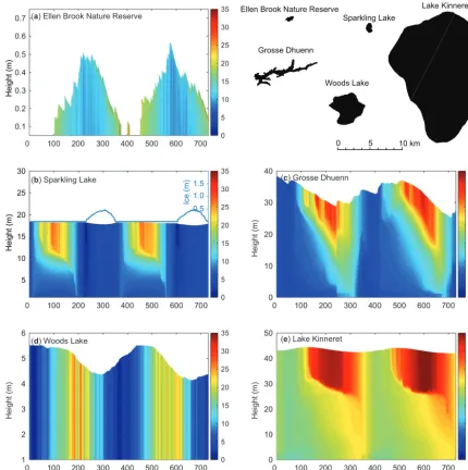
biogeochemists studying central basins of natural lakes (e.g. Gal et al., 2009), managers simulating drinking water reser-voirs (e.g. Weber et al., 2017), mining pit lakes (e.g. Salmon et al., 2017), or for analyses exploring the coupling between lakes and regional climate (e.g. Stepanenko et al., 2013). Further, whilst the model is able to resolve vertical strat-ification, the approach is also able to be used to simulate shallow lakes, wetlands, wastewater ponds, and other small waterbodies that experience well-mixed conditions. In this case, the layer resolution, with upper and lower layer bounds specified by the user, will automatically be reduced, and the mass of water, constituents, and energy will continue to be conserved. The remainder of this section outlines the model components and provides example outputs for five waterbod-ies that experience a diverse hydrology.
2.2 Water balance
The general nature of the model to accommodate a wide di-versity of lake types has necessitated flexibility in the config-uration of water inputs and outputs (schematically depicted in Fig. 1). The net water flux over the entire lake is summa-rized as
dVS dt =AS
dhS dt +
NINF
X
I
Qinf0I−
NOUTF
X
O
QoutfO
−Qseepage−Qovfl, (4)
sur-face, hS, are expanded upon below, and the remaining in-flow and outin-flow terms are described in detail in Sect. 7. For practical reasons the equation is numerically solved in two stages with different times steps for the surface flux change and all other fluxes. Furthermore, in any given application, not all the inputs and outputs are relevant and users may cus-tomize the water balance components accordingly; examples demonstrating lake hydrology from wetlands to reservoirs to deep lakes are presented in Fig. 2. Note that Eq. (4) accounts for the liquid water balance, and in cold climates the model will also track the amount of water allocated into an over-lying ice layer (Sect. 2.4), which interacts with the surface water balance as indicated next.
The mass balance of the surface layer is computed at each model time step (1t; usually hourly) by modifying the sur-face layer height,hS, according to
dhS
dt =RF+SF + QR AS
−E−d1zice
dt , (5)
where E is the evaporation mass flux computed from the latent heat fluxφE, described below (E=φE/λvρs; m s−1), RFis rainfall, andSFis snowfall (m s−1). Depending on the meteorological conditions, precipitation will either be added to the water volume or to the surface of the ice cover (see Sect. 2.4), andRF andSF therefore influence the water sur-face height depending on the presence of ice cover according to
RF=
(
fRRx/csecday if1zice=0
fRRx/csecday if1zice>0 andTa>0
0, if1zice>0 andTa≤0
(6)
and SF=
fSfSWESx/csecday if 1zice=0
0, if 1zice>0
. (7)
Here,fRandfSare user-defined scaling factors that may be applied to adjust the input data valuesRxandSx,
respec-tively. The surface height of the water column is also im-pacted by ice formation or melting of the ice layer sitting on the lake surface according to d1zice/dt, as described in Sect. 2.4.
QRis an optional term to account for run-off to the lake from the exposed riparian banks, which may be important in reservoirs with a large drawdown range or wetlands where periodic drying of the lake may occur. The run-off volume generated is averaged across the area that the active lake sur-face area (As) is not occupying, and the amount is calculated using a simple model based on exceedance of a rainfall in-tensity threshold,RL(m day−1), and run-off coefficient:
QR=max
0, fro RF−RLcsecday(Amax−AS) , (8)
wherefro is the run-off coefficient, defined as the fraction of rainfall that is converted to run-off at the lake’s edge, and Amaxis the maximum possible area of inundation of the lake (the area provided by the user as theNBSNvalue).
Note that mixing dynamics (i.e. the merging or splitting of layers to enforce the layer thickness limits) will impact the thickness of the surface mixed layer,zSML, but not change the overall lake height. However, in addition to the terms in Eq. (5),hSis modified due to volume changes associated with river inflows, withdrawals, seepage, or overflows, which are described in subsequent sections.
2.3 Surface energy balance
A balance of shortwave and longwave radiation fluxes and sensible and evaporative heat fluxes (all W m−2) determines the net cooling and heating across the surface. The general heat budget equation for the uppermost layer is described as cwρszs
dTs
dt =φSWS−φE+φH+φLWin−φLWout, (9) wherecwis the specific heat capacity of water,Tsis the sur-face temperature, and zs and ρs are the depth and density of the surface layer (i=NLEV), respectively. The right-hand side (RHS) heat flux terms are numerically computed at each time step and include several options for customizing the in-dividual surface heat flux components, which are expanded upon below.
2.3.1 Solar heating and light penetration
Solar radiation is the key driver of lake thermodynamics and may be input based on daily or hourly measurements from a nearby pyranometer. If data are not available then users may choose to have GLM compute surface irradiance from a the-oretical approximation based on the Bird Clear Sky Model (BCSM) (Bird, 1984) modified for cloud cover and latitude. The options for input are summarized as
φSW0 =
Option 1: daily insolation data provided
(1−αSW) fSWφSWxf[d, t− btc],
Option 2: sub-daily insolation data provided
(1−αSW) fSWφSWx,
Option 3: insolation computed from the BCSM
(1−αSW) fSWφˆSW,
(10a–c)
-200 -100 0 100 200 300 400 500 600 700 -8 -6 -4 -2 0 2 4 6 8 -4 -2 0 2 4 6 8 10 12 14
(a) Ellen Brook Nature Reserve
(c) Grosse Dhuenn
Total inflow Total outflow Net water flux
12 8 0 -4 4 700 600 0 -200 500 400 300 200 100 -100 -4 -2 0 2 4 6 8 6 0 -4 2 4 10 -2 V ol um e flu x ( x 10 M L d ) 6 -1 V ol um e flu x ( x 10 M L d ) 5 -1 V ol um e flu x ( M L d ) -1
0 5 10 km
Ellen Brook Nature Reserve
Sparkling Lake Lake Kinneret Grosse Dhuenn Woods Lake -3 -2 -1 0 1 2 3 3 1 -2 -3 0 2 -1
(b) Sparkling Lake
(d) Woods Lake 6 2 -6 -8 0 4 -4 -2 8
0 100 200 300 400 500 600 700 Simulation days V ol um e flu x ( x 10 M L d ) 5 -1
0 100 200 300 400 500 600 700 Simulation days V ol um e flu x ( x 10 M L d ) 4 -1 Evaporation Rainfall & snow River inflow Seepage Overflow Withdrawal Submerged inflow Local run-off
(e) Lake Kinneret
Figure 2.A 2-year times series of the simulated daily water balance for five example lakes(a–e)that range in size and hydrology. The water balance components summarized are depicted schematically in the inset and partitioned into inputs and outputs. The daily net water flux is computed from Eq. (4). For more information about each lake, the simulation configuration, and input data, refer to the “Data availability” section.
option 3 the BCSM is used (Bird, 1984; Luo et al., 2010):
ˆ φSW=
ˆ
φDB+ ˆφAS
1−(αSWαSKY)f[Cx], (11) where the total irradiance, φSW, is computed from directˆ beamφDBˆ and atmospheric scatteringφASˆ components (refer to Appendix A for a detailed outline of the BCSM equations and parameters). In GLM, the clear-sky value is then reduced according to the cloud cover data provided by the user,Cx,
according to
f[Cx]=0.66182Cx2−1.5236Cx+0.98475, (12)
which is based on a polynomial regression of cloud data from Perth Airport, Australia, compared against nearby
sen-sor data (R2=0.952; see also a similar relationship by Luo et al., 2010).
Option 1 : daily approximation from Hamilton and Schladow (1997)
αSW=
αSWmean−δαSWsin
2π
365d− π 2
:northern hemisphere,Lat>0 αSWmean
:equator αSWmean−δαSWsin
2π
365d+ π 2
:southern hemisphere,Lat<0
(13a)
Option 2: sub-daily approximation from Briegleb et al. (1986)
αSW= 1 100
2.6
cos [8zen]1.7+0.065
+15(cos [8zen]−0.1)
(cos [8zen]−0.5) (cos [8zen]−1)
(13b) Option 3: sub-daily approximation from Yajima
and Yamamoto (2015) αSW=max
h
0.02,0.001fRHRHx(1−cos [8zen])0.33 −0.001U10(1−cos [8zen])−0.57−0.001ς
(1−cos [8zen])0.829i (13c)
Option 4: daily approximation from Grischenko look-up table in Cogley (1979)
αSW=αSWG[Lat, d] (13d)
Here,8zenis the solar zenith angle (radians) as outlined in Appendix A, RHxis the relative humidity,ςis the percentage
of atmospheric diffuse radiation,dis the day of year, andU10 is wind speed. The second (oceanic) and third (lacustrine) options are included to allow for diel and seasonal variation of albedo from approximately 0.01 to 0.4 depending on the sun angle (Fig. 3). Option 4 may be better for higher-latitude sites; also note that albedo is calculated separately during ice cover conditions using a customized algorithm, as outlined below in Sect. 2.4.
The depth of penetration of shortwave radiation into the lake is wavelength specific and depends on the water clar-ity via the light extinction coefficient, Kw (m−1). Two ap-proaches are supported in GLM. The first option assumes that the photosynthetically active radiation (PAR) fraction of the incoming light is the most penetrative and follows the Beer– Lambert law:
φPAR[z]=fPARφSW0exp [−Kwz], (14)
where z is the depth of any layer from the surface. Kw may be set by the user as constant, read in from a time se-ries file, or linked with the water quality model (e.g. FABM
Figure 3.Variation of albedo (αSW) with solar zenith angle (SZA
=8zen180/π, degrees) for options 2 and 3 (Eq. 13). For option 3,
settings of RHx=80 % andU10=6 m s−1were assumed.
or AED2; see Sect. 4); in the latter case the extinction co-efficient will change as a function of depth and time ac-cording to the concentration of dissolved and particulate constituents. For this option Beer’s law is only applied for the photosynthetically active fraction,fPAR, which is set as 45 % of the incident light. The amount of radiation heat-ing the surface layer,φSWS, is therefore the
photosyntheti-cally active fraction that is attenuated acrosszs, plus the en-tire(1−fPAR)fraction,φSWS=φSW0−φPAR[zs], which
im-plicitly assumes that the near-infrared and ultraviolet band-widths of the incident shortwave radiation have significantly higher attenuation coefficients (Kirk, 1994). The second op-tion adopts a more complete light absorpop-tion algorithm that integrates the attenuated light intensity across the bandwidth spectrum:
cwρi1zi
dTi
dt =
NSW
X
l=1
φSWil[zi]− NSW
X
l=1 φSWi−1l
zi−1, (15)
wherelis the bandwidth index andφSWil[zi] is the radiation
flux at the top of theith layer for thelth bandwidth fraction. For this option, the model by Cengel and Ozisk (1984) is adopted to compute the penetration of individual bandwidth fractions, which more comprehensively resolves the incident and diffuse radiation components of the light climate, taking into account the angle of incident light, transmission across the light surface (based on the Fresnel equations), and reflec-tion off the bottom. These processes are wavelength specific and the user specifies the number of simulated bandwidths, NSW, their respective absorption coefficients,Kwl, and
re-flectivity of light at the sediment,αsed.
for the type of benthic habitat that might emerge. In addition to the light profiles, GLM therefore predicts the benthic area of the lake in which light intensity exceeds a user-defined fraction of the surface irradiance,fBENcrit, (Fig. 4):
ABEN=AS−A[hBEN], (16)
wherehBEN=hS−zBEN,zBENis calculated from Beer’s law,
zBEN= −
lnfBENcrit
Kw , (17)
and the daily average benthic area above the threshold is then reported as a percentage (100×ABEN/As).
2.3.2 Longwave radiation
Longwave radiation can be provided as a net flux, an incom-ing flux, or, if there are no radiation data from which long-wave radiation can be computed, then it may be calculated by the model internally from the cloud cover fraction and air temperature. Net longwave radiation is described as
φLWnet=φLWin−φLWout, (18)
where
φLWout=εwσ (θs)
4; (19)
σ is the Stefan–Boltzmann constant andεwthe emissivity of the water surface, assumed to be 0.985. If the net or incoming longwave flux is not provided, the model will compute the incoming flux from
φLWin=(1−αLW) ε
∗
aσ (θa)4, (20)
whereαLWis the longwave albedo (0.03). The emissivity of the atmosphere can be computed considering emissivity for cloud-free conditions (εa) based on air temperature (Ta) and vapour pressure and extended to account for reflection from clouds such thatε∗a=f[Ta, ea, Cx] (see Henderson-Sellers,
1986; Flerchinger et al., 2009). Options adapted from a range of authors include the following:
εa∗=
Option 1:Idso and Jackson(1969)
(1+0.275Cx) 1−0.261 exp−0.000777Ta2
,
Option 2:Swinbank(1963)
1+0.17C2
x
9.365×10−6(θ a)2,
Option 3:Brutsaert(1975)
(1+0.275Cx)1.24(ea/θa)1/7,
Option 4:Yajima and Yamamoto(2015)
1−C2.796
x
1.24(ea/θa)1/7+0.955Cx2.796,
(21a–d)
whereCx is the cloud cover fraction (0–1) and ea the air
vapour pressure calculated from relative humidity. Note that cloud cover is typically reported in octals (0–8), and thus a value of 1 would correspond to a fraction of 0.125. Some data may also include cloud type and their respective heights. If this is the case, good correspondence has been reported by averaging the octal values for all cloud types to get an aver-age cloud cover.
If longwave radiation data do not exist and cloud data are also not available, but solar irradiance is measured, then GLM rad_mode setting 3 will instruct the model to compare the measured and theoretical clear-sky solar irradiance (esti-mated by the BCSM; Eq. 11) to approximate the cloud cover fraction by assuming thatφSWx/φSWˆ =f[Cx]. Note that if
neither shortwave or longwave radiation is provided, then the model will use the BCSM to compute incoming solar irradi-ance, and cloud cover will be assumed to be 0 (noting that this is likely to overestimate downwelling shortwave radia-tion).
2.3.3 Sensible and latent heat transfer
The model accounts for the surface fluxes of sensible heat and latent heat using commonly adopted bulk aerodynamic formulae. For sensible heat,
φH= −ρacaCHU10(Ts−Ta) , (22) where ca is the specific heat capacity of air, CH is the bulk aerodynamic coefficient for sensible heat transfer,Ta the air temperature, and Ts the temperature of the water surface layer. The air density (kg m−3) is computed from ρa=0.348(1+r)/(1+1.61r) p/Ta, wherepis air pressure (hPa) andris the water vapour mixing ratio, which is used to compute the gas constant.
For latent heat, φE= −ρaCEλvU10
ω
p (es[Ts]−ea[Ta]) , (23) whereCEis the bulk aerodynamic coefficient for latent heat transfer,eathe air vapour pressure,es the saturation vapour pressure (hPa) at the surface layer temperature (◦C),ω the ratio of the molecular mass of water to the molecular mass of dry air (=0.622), andλvthe latent heat of vaporization. The vapour pressure is calculated by the linear formula from Tabata (1973):
es[Ts]=10
9.28603523−2322.37885 Ts+273.15
(24) and
Figure 4.Example light data outputs from a GLM application to Woods Lake, Australia, showing(a)the ratio of benthic to surface light, 100φPARBEN/φSW0(%), overlain on the lake map based on the bathymetry, with the area wherefBENcrit<0.2 (i.e. less than 20 % of surface
irradiance) depicted in grey,(b)a time series of the depth variation in light (W m−2), and(c)a time series ofABEN/As(as %) for various
fBENcrit. Note that the 2-D projection of the 1-D lake model in(a)can assist in managing the lake condition but assumes uniformity ofKw.
Correction for non-neutral atmospheric stability
For long time integrations (e.g. seasonal), the bulk-transfer coefficients for momentum, CD, sensible heat, CH, and la-tent heat, CE, can be assumed approximately constant be-cause of the negative feedback between surface forcing and the temperature response of the waterbody (e.g. Strub and Powell, 1987). At finer timescales (hours to weeks), the ther-mal inertia of the waterbody is too great, so the transfer co-efficients should be specified as a function of the degree of atmospheric stratification experienced in the internal bound-ary layer that develops over the water (Woolway et al., 2017). Monin and Obukhov (1954) parameterized the stratification in the air column using the now well-known stability param-eter,z/L, which is used to define corrections to the bulk aero-dynamic coefficientsCHandCEusing the numerical scheme presented in Appendix B. The corrections may be optionally applied within a simulation, and if enabled, the transfer coef-ficients used above are automatically updated. To ensure that the data provided are from within the internal boundary layer over the lake surface, users should preferably provide wind speed, air temperature, and relative humidity data that have been collected over the lake surface (at a height of 2–10 m, depending on lake size), supplied at approximately hourly resolution.
Wind sheltering
Wind sheltering may be important depending on the lake size and shoreline complexity and is parameterized according to several methods based on the context of the simulation and data available. For example, Hipsey and Sivapalan (2003) presented a simple adjustment to the bulk-transfer equation to account for the effect of wind sheltering in small
reser-voirs using a shelter index to account for the length scale associated with the vertical obstacle relative to the horizon-tal length scale associated with the waterbody itself. Mark-fort et al. (2010) estimate the effect of a similar sheltering length scale on the overall lake area calculated based on sur-rounding topography and canopy heights relative to the water surface. Therefore, within GLM, users may specify the de-gree of sheltering or fetch limitation using either constant or direction-specific options for computing an “effective” area. AE=
Option 0: no sheltering (default) AS,
Option 1: Yeates and Imberger (2003)
AStanh
A
S AWS
,
Option 2: Markfort et al. (2010) L2D
2 arccos
"
xWS8 LD
#
−x 8
WS 2
q
L2D− xWS8 2,
Option 3: user-defined shelter index fWS[8wind]AS,
(26a–d)
based on the size of the lake, whereas options 2 and 3 require users to additionally input wind direction data and a direc-tion funcdirec-tion,fWS[8wind], to allow for a variable sheltering effect over time. In the case of option 2, this function scales the sheltering distance,xWS, as a function of wind direction, xWS8 =xWS(1−min(fWS[8wind],1)), whereas in the case of option 3 the function reads in an effective area scaling fraction directly based on a precalculated shelter index.
The ratio of the effective area to the total area of the lake, AE/AS, is then used to scale the wind speed data input by the user,Ux, as a means of capturing the average wind speed
over the entire lake surface such that U10=fUUxAE/AS,
wherefU is a wind speed adjustment factor that can be used
to assist calibration or to correct the raw wind speed data to the reference height of 10 m.
Still-air limit
The above formulations apply when sufficient wind exists to create a defined boundary layer over the surface of the water. As the wind tends to zero (the “still-air limit”), Eqs. (22)– (23) become less appropriate as they do not account for free convection directly from the water surface. This is a rela-tively important phenomenon for small lakes, cooling ponds, and wetlands since they tend to have small fetches that limit the energy input from wind. These waterbodies may also have large areas sheltered from the wind and will develop surface temperatures warmer than the atmosphere for con-siderable periods. Therefore, users can optionally augment Eqs. (22)–(23) with calculations for low wind speed condi-tions by calculating the evaporative and sensible heat flux values for both the given U10 and for an assumed U10=0. The chosen value for the surface energy balance (as applied in Eq. 9) is found by taking the maximum value of the two calculations:
φX∗ =
Option 1: no-sheltering area maxφX, φX0
Option 2: still-air sheltered area max
φX, φX0
AE/AS+φX0(AS−AE) /AS
, (27)
whereφX0 is the zero-wind flux for either the evaporative or
sensible heat flux (φE0 andφH0, respectively) andφXis
cal-culated from Eqs. (22)–(23). The two zero-wind-speed heat flux equations are from TVA (1972), but modified to return energy flux in SI units (W m−2).
φE0=ρsλvαe(ϑs−ϑa) (28a)
φH0 =αh(Ts−Ta) (28b)
αe=0.137f0 Kair caρs
g|ρa−ρo| ρaνaDa
1/3
(29a)
αh=0.137f0Kair
g|ρa−ρo| ρaνaDa
1/3
(29b)
Here,ν=κ e/p, with the appropriate vapour pressure val-ues,e,for both surface and ambient atmospheric values.Kair is the molecular heat conductivity of air (J m−1s−1C−1),νa is the kinematic viscosity of the air (m2s−1),ρois the
den-sity of the saturated air at the water surface temperature,ρsis the density of the surface water,f0is a dimensionless rough-ness correction coefficient for the lake surface, andDais the molecular heat diffusivity of air (m2s−1). Note that the im-pact of low wind speeds on the drag coefficient is captured by the modified Charnock relation (Eqs. B2–B3), which in-cludes an additional term for the smooth flow transition (see also Fig. A1).
2.4 Snow and ice dynamics
The extent of ice and snow cover can significantly impact the lake water balance and mixing regime depending on the pre-vailing environmental conditions. The algorithms for GLM ice and snow dynamics are based on previous ice modelling studies that adopt a three-layer scheme for resolving ice and snow split into blue ice (or black ice), white ice (or snow ice), and snow layers (Patterson and Hamblin, 1988; Gu and Stefan, 1993; Rogers et al., 1995; Vavrus et al., 1996; Launiainen and Cheng, 1998; Magee et al., 2016). Blue ice is formed through direct freezing of lake water into ice, whereas white ice is generated in response to seeping of lake water onto the ice surface when the mass of snow that can be supported by the buoyancy of the ice cover is exceeded (see below; Rogers et al., 1995). The snow layer is subject to compaction and melting based on surface meteorological conditions and the ice layers are affected by the lake water temperature at the lower boundary.
Blue ice initially forms when the water at the lake surface goes below 0◦C. Once fresh snow deposits on the surface it is subject to densification, which depends on the air tem-perature and amount of rainfall (Fig. 6); the density of fresh snowfall is determined as the ratio of measured snowfall height to water-equivalent height, with any values exceed-ing the assigned maximum or minimum snow density (de-faults: ρs,max=300 kg m−3, ρs,min=50 kg m−3) truncated to the appropriate limit. The snow compaction equation is based on the exponential decay formula of McKay (1968), with the selection of snow compaction parameters based on air temperature and depending on whether rainfall or snow-fall is being added. When the weight of snow exceeds the buoyancy of the ice layer,
1zsnowρsnow>{1zblue(ρw−ρblue)
0 100 200 300 400 500 600 700 -500
-250 0 250 500
0 100 200 300 400 500 600 700
-500 -250 0 250 500
0 100 200 300 400 500 600 700
-500 -250 0 250 500
Heat balance Heat balance (weekly) 500
250
-250
-500 0
500 250
-250 -500 0
500 250
-250 -500 0
500 250
-250 -500 0
Heat flux (W m
)
-2
0 100 200 300 400 500 600 700
-500 -250 0 250 500
500 250
-250 -500 0
0 100 200 300 400 500 600 700
-500 -250 0 250 500
500 250
-250 -500 0
0 100 200 300 400 500 600 700 0 100 200 300 400 500 600 700 Simulation days
Simulation days
0 5 10 km
Ellen Brook Nature Reserve
Sparkling Lake
Lake Kinneret
Grosse Dhuenn
Woods Lake zsml (1−αLW)φLWin
φLWin
αLWφLWφLWout
φE φH
u*
U(z)
ΦΖΕΝ φSW
(1−αSW)φSW
φSW
S
αSWφSW
Ux , T , RHa
Ts
φsw X
-φSW 0 S
(a) Ellen Brook Nature Reserve
(c) Grosse Dhuenn (b) Sparkling Lake
(d) Woods Lake (e) Lake Kinneret
φSW
φH
φLW
φE 0
Dry Dry
Heat flux (W m
)
-2
Heat flux (W m
)
-2
Heat flux (W m
)
-2
Heat flux (W m
)
-2
Figure 5.A 2-year times series of the simulated daily heat fluxes for the five example lakes(a–e)that were depicted in Fig. 2. The heat balance components summarized are depicted schematically in the inset, as described in Sect. 2.3, and the “heat balance” line refers to the LHS of Eq. (9).
To capture the changing thickness of the ice and snow lay-ers due to melting or freezing, the model employs a quasi-steady-state assumption to solve the heat transfer equation through the layers by assuming that the timescale for heat conduction is short relative to the timescale of changes in me-teorological forcing (Patterson and Hamblin, 1988; Rogers et al., 1995). By assigning appropriate boundary conditions at the ice–atmosphere and ice–water interfaces, the model com-putes the upward conductive heat flux through the ice and snow cover to the atmosphere, termedφ0.
At the upper surface (which could be ice or snow), a heat flux balance is employed to provide the condition for surface melting:
φ0[T0]+φnet[T0]=0 T0< Tm, (31) φnet[T0]= −ρice,snowλf
d1zice,snow
dt , (32)
whereλfis the latent heat of fusion,1zice,snowis the height of either the upper snow or ice layer,ρice,snowis the density of the relevant snow or ice layer determined from the surface medium properties,T0is the temperature at the solid surface, andTm is the meltwater temperature (0◦C).φnet[T0] is the net incoming heat flux for non-penetrative radiation at the solid surface:
φnet[T0]=φLWin−φLWout[T0]+φH[T0]
+φE[T0]+φR[T0], (33) where the heat fluxes between the solid bound-ary and the atmosphere are calculated as out-lined previously, but with modification for the de-termination of vapour pressure over ice or snow (esice[T0]=es[T0] 1+9.72×10
−3T
0+4.2×10⁻⁵T02
( Dzsnow= 0)
( Dzsnow> 0)
( *S
F> 0)
( *R
F> 0; *SF= 0)
( *S
F> 0)
( *R
F> 0; *SF= 0)
( *R
F= 0; *SF= 0)
Dzsnow= *SF Dt ; rsnow= rs-min
Dzsnow= *SFDt; rsnow= rw*RF / *SF
RF= *RF
Dzsnow= *RF Dt /fswe; rsnow=rs-max
*R
F= min[ *RF , fswe*SF]Dt fsnow= 0.166+0.834(1-e-*RF)
*R
F= min[RF, fswe*SF]Dt fsnow= 0.088+0.912(1-e-lsnow)
fsnow= 0.088 fsnow= 0.166
fsnow= 0.166+0.834(1-e-lsnow); rsnow* =rsnow+ fsnow(rs-max-rsnow)
Dzsnow=Dzsnow(rsnow/rsnow*) RF= *RF
*S
F= *RF/ (rs-max/rw)
Dzsnow=Dzsnow(rsnow/rs-max) + *SFDt
rsnow=rs-max
rsnow* =rsnow+ fsnow(rs-max-rsnow)
Dzsnow=Dzsnow(rsnow*/rsnow)
( *R
F= 0; *SF= 0) RF = 0
RF > 0
Ta> 0
Ta < 0
Ta > 0
Ta < 0 Ta> 0
Ta < 0 Ta> 0
Ta < 0
rsnow* =rsnow+ fsnow(rs-max-rs-old)
Dzsnow*=Dzsnow(rsnow/rsnow*)
rsnow=(rsnow*Dzsnow* +*RFDt)/(Dzsnow* + *SFDt) Dzsnow=Dzsnow*+ *SFDt
Dzblue Dzwhite Dzsnow
ff f0 fnet
fw fSW0 b
a
dwi
Ice on
Ice-covered
Snow & Ice-covered
Snowfall
Rainfall
Snowfall
Rainfall
No precipitation
Rainfall added to lake:
No change
Rainfall added to lake: No precipitation
water
Snow compaction
( ) ( )
i
Figure 6. (a)Decision tree describing updates to the snow cover each time step according to the amount of incident rainfall (∗RF) and
snowfall (∗SF), air temperature (Ta), and snow compaction rules.(b)Schematic of ice and snow layers and heat fluxes. Refer to the text and
Table 1 for definitions of other variables. Here,∗RF=fRRx/csecdayand∗SF=fSSx/csecdayif ice cover is present; otherwise they are set
to 0 and the model reverts to Eqs. (6)–(7).
(φR=∗RFρwλf to capture the freezing effect if T0< Tm or simply as ∗RFcwρw(Ta−T0) if T0=Tm; Rogers et al., 1995). To determine the flow of heat through the layers, Rogers et al. (1995) derived the following.
3 φ0−φSW0=Tm−T0
− (
fVISφSW0
1−e−Ks11zsnow
KsnowKs1
+e−Ks11zsnow 1−e
−Kw11zwhite
Kw11zwhite +e
−Ks11zsnow−Kw11zwhite
1−e−Kb11zblue
Kb11zblue
!)
− (
(1−fVIS) φSW0
1−e−Ks21zsnow
KsnowKs2
+e−Ks21zsnow 1−e
−Kw21zwhite
Kw21zwhite +e−Ks21zsnow−Kw21zwhite 1−e
−Kb21zblue
Kb21zblue
!)
+φsi1zsnow3−φsi1z 2 snow 2Ksnow
(34)
Here,3=1zsnow
Ksnow +
1zwhite
Kwhite +
1zblue
Kblue
,φSW0is the shortwave radiation penetrating the ice–snow surface, K refers to the
light attenuation coefficient of the ice and snow components designated with subscripts s, w, and b for snow, white ice, and blue ice, respectively, and the1zterms refer to the thick-ness of snow, white ice, and blue ice. This is rearranged and solved forT0andφ0by using a bilinear iteration until surface heat fluxes are balanced (i.e.φ0[T0]= −φnet[T0]) andT0is stable (±0.001◦C). In the presence of ice (or snow) cover,
a surface temperatureT0> Tmindicates that energy is avail-able for melting. The amount of energy for melting is calcu-lated by settingT0=Tmto determine the reduced thickness of snow or ice (as shown in Eq. 32). The estimation ofφ0 applies an empirical equation to estimate snow conductivity, Ksnow, from its density (Ashton, 1986):
Ksnow=0.021+0.0042ρsnow+(2.2×10⁻⁹ρsnow3 ). (35) The heat flux in the ice at the ice–water interface is
φf=φ0 −fVISφSW0 (1−exp [−Ks11zsnow−Kw11zwhite
and snow light attenuation coefficients in GLM are also fixed to the same values as those given by Rogers et al. (1995). Shortwave albedo for the ice or snow surface (required for Eq. 10) is a function of surface medium (see Table 1 of Vavrus et al., 1996) with values varying from 0.08 to 0.6 for ice and from 0.08 to 0.7 for snow, depending on the surface temperature and the layer thicknesses; an additional scaling factor for the snow albedo, fα, is also implemented to aid
calibration.
Accretion or ablation of blue ice occurs at the ice–water boundary based on the conductive heat flux from water into the ice,φw, as given by the finite-difference approximation: φw= −Kwater
1T
δwi , (37)
whereKwateris the molecular conductivity of water (assum-ing the water is stagnant under the ice), and1T is the tem-perature difference between the surface water of the lake and the bottom of the blue ice layer,Tm−Ts. This occurs across an assigned length scale,δwi, for which a value of 0.1–0.5 m is usual based on the reasoning given in Rogers et al. (1995) and the typical vertical water layer resolution of a model simulation (0.125–1.5 m). Note that a wide variation in tech-niques and values is used to determine the basal heat flux immediately beneath the ice pack (e.g. Harvey, 1990), which suggests that this may need careful consideration during cal-ibration.
The imbalance between φf moving through the blue ice layer and the heat flux from the water into the ice,φw, gives the rate of change of ice thickness at the interface with water:
d1zblue
dt =
φf−φw ρblueλf
. (38)
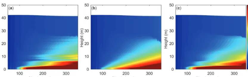
The ice thickness is set to its minimum value of 0.05 m, which is suggested by Patterson and Hamblin (1988) and Vavrus et al. (1996). The need for a minimum ice thickness relates primarily to horizontal variability of the ice cover dur-ing formation and closure (ice-on) periods. The ice cover equations are discontinued and open water conditions are re-stored in the model when the thermodynamic balance first produces ice thickness<0.05 m. Example outputs are shown in Fig. 7; see also Yao et al. (2014) for a previous application. 2.5 Sediment heating
The water column thermal budget may also be affected by heating or cooling from the soil–sediment below. For each layer, the rate of temperature change depends on the temper-ature gradient and the relative area of the layer volume in contact with bottom sediment:
cwρi1Vi
dTi
dt =Ksoil
Tzi−Ti
δzsoil
(Ai−Ai−1) , (39)
where Ksoil is the soil–sediment thermal conductivity and δzsoil is the length scale associated with the heat flux. The
temperature of the bottom sediment varies seasonally and also depending on its depth below the water surface such that
Tzi=Tzmean+δTzcos
2π
365 d−dTz
, (40)
wherezis the soil–sediment zone that theith layer overlays (see Sect. 4 for details),Tz is the temperature of this zone,
Tzmean is the annual mean sediment zone temperature,δTzis
the seasonal amplitude of the sediment temperature variation, anddTzis the day of the year when the sediment temperature
peaks. By defining different sediment zones, the model can therefore allow for a different mean and amplitude of littoral waters compared to deeper waters. A dynamic sediment tem-perature diffusion model is also under development, which will be suitable when empirical data for the above parame-ters in Eq. (40) are not available.
2.6 Stratification and vertical mixing
Mixing processes in lakes are varied and depend upon the degree of meteorological and hydrological forcing, the lake morphometry, and the nature of thermal stratification expe-rienced by the lake at the time of forcing. Numerous mod-els adopt an eddy-diffusivity approach whereby mixing is captured using the advection–dispersion equation (e.g. Ri-ley and Stefan, 1988). GLM adopts an energy balance ap-proach as used in DYRESM whereby the mixing dynamics are based on estimating the amount of turbulent energy avail-able, which is separately computed for the surface mixed layer (surface mixing) and for mixing below the thermocline (deep mixing).
2.6.1 Surface mixed layer
To compute mixing of layers, GLM works on the premise that the balance between the available energy, ETKE, and the energy required for mixing to occur, EPE, provides the surface mixed layer (SML) deepening rate dzSML/dt, where zSML is the depth from the surface to the bottom of the surface mixed layer. For an overview of the dynam-ics, readers are referred to early works on bulk mixed layer depth models by Kraus and Turner (1967) and Kim (1976), which were subsequently extended by Imberger and Patter-son (1981) and Spigel et al. (1986) as a basis for hydrody-namic model design. Using this approach, the available ki-netic energy is calculated due to contributions from wind stir-ring, convective overturn, shear production between layers, and Kelvin–Helmholtz (K–H) billowing. Overall, the turbu-lent energy generated for mixing is summarized as (Hamilton and Schladow, 1997)
ETKE=0.5CK(w∗3)1t
| {z }
convective overturn
+0.5CK(CWu3∗)1t
| {z }
wind stirring
Figure 7.Example of modelled and observed thickness of(a)blue ice,1zblue,(b)white ice,1zwhite, and(c)snow,1zsnow, for Sparkling
Lake, Wisconsin. Points are the average observed thicknesses.
+0.5CS
"
u2b+u 2 b 6
dδKH dzSML+
ubδKH 3
dub dzSML
#
| {z }
shear production K–H production
1zk−1,
whereδKHis the K–H billow length scale (described below), ubis the shear velocity at the interface of the mixed layer, and CK, CW, and CS are mixing efficiency constants. For mixing to occur, the energy must be sufficient to lift up water in the layer below the bottom of the mixed layer, denoted here as the layerk−1 with thickness1zk−1, and accelerate
it to the mixed layer velocity,u∗. This must also account for
energy consumption associated with K–H billowing. In total, the energy required to entrain a layer into the mixed layer is expressed asEPE:
EPE=
0.5CT(w∗3+CWu3∗)
2/3
| {z }
acceleration
+1ρ ρo
gzSML
| {z }
lifting
+gδ 2 KH 24ρo
d(1ρ) dzSML +
gδKH1ρ 12ρo
dδKH dzSML
| {z }
K–H consumption
1zk−1, (42)
whereCTis a mixing efficiency constant to account for un-steady turbulence. To numerically resolve Eqs. (41) and (42) the model sequentially computes the different components of the above expressions with respect to the layer structure, thereby checking the available energy relative to the required amount (depicted schematically in Fig. 8). GLM follows the sequence of the algorithm presented in detail in Imberger and Patterson (1981), whereby layers are combined due to con-vection and wind stirring first, and then the resultant mixed layer properties are used when subsequently computing the extent of shear mixing and the effect of K–H instabilities. Plots indicating the role of mixing in shaping the thermal structure of the example lakes are shown in Fig. 9.
To compute the mixing energy available due to convec-tion, in the first step, the value forw∗ is calculated, which
brought about by cooling at the air–water interface. The model adopts the algorithm used in Imberger and Patter-son (1981), whereby the potential energy that would be re-leased by mixed layer deepening is computed from the first moment of layer masses in the epilimnion (surface mixed layer) about the lake bottom relative to the well-mixed con-dition. This is numerically computed by summing from the bottom-most layer of the epilimnion,k, up toNLEV:
w∗3=
g ρSML1t NLEV X i=k h
(ρi1zi)
e
hi−h]SML
i
, (43)
whereρSMLis the mean density of the mixed layer including the combined layer,ρi is the density of theith layer,1zi is
the height difference between two consecutive layers within the loop (1zi=hi−hi−1),hei is the mean height of layers to
be mixed (hei =0.5[hi+hi−1]), andh]SML is the epilimnion mid-height calculated ash]SML=0.5(hS+hk−1), wherehS is the height of the surface water level.
The velocity scaleu∗of the surface layer is associated with
wind stress and calculated according to the wind strength: u2∗=
ρa ρSML
CDU102, (44)
whereCDis the drag coefficient for momentum. The model first checks to see if the energy available (Eqs. 43 and 44) can overcome the energy required to mix thek−1 layer into the surface mixed layer (Fig. 8e); i.e. mixing ofk−1 occurs if CK
w3∗+CWu3∗
1t ≥
gk0zSML+CT
w3∗+CWu3∗ 2/3
1zk−1, (45)
where gk0=g1ρ
ρo is the reduced gravity between
the mixed layer and the k−1 layer calculated as g (ρSML−ρk−1) /(0.5(ρSML+ρk−1)). If the mixing condition is met, the layers are combined, the energy required to combine the layer is removed from the available energy, k is adjusted, and the loop continues to the next layer. When the mixing energy is substantial and the mixing reaches the bottom layer, the mixing routine ends. If the condition in Eq. (45) is not met, then any residual energy is stored for the next time step, and the mixing algorithm continues as outlined below.
Once stirring is completed, mixing generated due to veloc-ity shear is then accounted for. Parameterizing the shear ve-locity, denotedub, in a one-dimensional model can be prob-lematic; however, the approximation used in Imberger and Patterson (1981) is applied:
ub=
u2∗1t
zSML
+ubold, t≤tb+δtshear
0, t > tb+δtshear
, (46)
where ubold is from the previous time step and zeroed
be-tween shear (wind) events. Therefore, this model yields a
simple linear increase in the shear velocity over time for a constant wind stress. This is considered relative toδtshear, which is the cut-off time beyond which it is assumed that no further shear-induced mixing occurs for that event. This cut-off time assumes the use of only the energy produced by shear at the interface during a period equivalent to half the basin-scale seiche duration,δtiw, which can be modified to account for damping (Spigel, 1978):
δtshear= (47)
1.59δtiw
δtdamp δtiw
≥10
1+0.59 1−cosh
δtdamp δtiw
−1 −1!!
δtiw
δtdamp δtiw
<10,
where δtdamp is the timescale of damping. The wave pe-riod is approximated based on the stratification as δtiw= LMETA/2c, where LMETA is the length of the basin at the thermocline calculated from √Ak−1(4/π ) (Lcrest/Wcrest), whereby an ellipse shape is assumed and cis the internal wave speed,
c= s
|gEH0|
δepiδhyp δepi+δhyp
, (48)
whereδepi andδhyp are characteristic vertical length scales associated with the epilimnion and hypolimnion:
δepi=
1Vepi 0.5(As+Ak−1)
;δhyp= Vk−1 0.5Ak−1
, (49)
where1VepiandVk−1are the associated volumes.
The time for damping of internal waves in a two-layer sys-tem can be parameterized by estimating the length scale of the oscillating boundary layer, through which the wave en-ergy dissipates, and the period of the internal standing wave (see Spigel and Imberger, 1980):
δtdamp=
√
νw
cdampδss
2 δepi+δhyp
u2
∗ r
c 2LMETA
δhyp
δepi
δepi+δhyp
. (50) Once the velocity is computed from Eq. (46), the energy for mixing from velocity shear is compared to that required for lifting and accelerating the next layer down, and layers are combined if there is sufficient energy (Fig. 6f), i.e. when
0.5CS
"
u2b zSML]+1δKH
6 +
ubδKH1ub 3
#
+
gk0δKH
δKH1z k−1 24zSML − 1δKH 12 ≥
gk0zSML+CT
w3∗+CWu3∗ 2/3
1zk−1, (51)
is computed from the difference between the bulk epilimnion and hypolimnion waters (Eq. 49), andCKH is a measure of the billow mixing efficiency.
Once energy from shear mixing is exhausted, the model checks the resultant density interface to see if it remains un-stable to shear such that K–H billows would be expected to form, i.e. if the metalimnion thickness is less than the K–H length scale,δKH. If this condition is met, a six-layer set is created about the thermocline to relax the stratification, set to have a linear density profile overδKH (Fig. 8g), and the surface layer properties are updated.
2.6.2 Deep mixing
Mixing below the thermocline in lakes, in the deeper hy-polimnion, is modelled using a characteristic vertical diffu-sivity,DZ=Dε+Dm, whereDmis a constant molecular
dif-fusivity for scalars andDεis the turbulent diffusivity. Three
hypolimnetic mixing options are possible in GLM including (1) no diffusivity, DZ=0, (2) a constant vertical
diffusiv-ityDZ over the water depth below the surface mixed layer,
or (3) a derivation by Weinstock (1981) used in DYRESM, which is described as being suitable for regions displaying weak or strong stratification, whereby diffusivity increases with dissipation and decreases with heightened stratification. For the constant vertical diffusivity option, the coefficient CHYP is interpreted as the vertical diffusivity (m2s−1), i.e. Dz=CHYP, and applied uniformly below the surface mixed layer. For the Weinstock (1981) model, the diffusivity varies depending on the strength of stratification and the rate of tur-bulent dissipation according to
Dz=
CHYPεTKE N2+0.6k
TKE2u∗2
, (52)
whereCHYPin this case is the mixing efficiency of hypolim-netic TKE (∼0.8 in Weinstock, 1981),kTKEis the turbulence wavenumber defined below, andu∗is defined as above. The
stratification strength is computed using the Brunt–Väisälä (buoyancy) frequency,N2, defined for a given layerias Ni2=g1ρ
ρ1z≈
g (ρi−2−ρi+2)
ρref(hi+2−hi−2)
, (53)
whereρrefis the average of the layer densities. This is com-puted from layer three upwards, averaging over the span of five layers until the vertical density gradient exceeds a set tolerance.N2varies following an approximate normal distri-bution with height, centred at the height at which the centre of buoyancy is located and computed each time step from the first moment of the vertical N2 distribution. Addition-ally, GLM estimates the vertical length scale associated with 1 standard deviation about the centre of theN2distribution, denotedδzσ.
The diffusivity increases in line with the turbulent dissipa-tion rate. This can be complex to estimate in stratified lakes;
however, GLM adopts a simple approach as described in Fis-cher et al. (1979) in which a “net dissipation” is approxi-mated by assuming that dissipation is in equilibrium with energy inputs from external forcing:
εTKE≈εTKE=εWIND+εINFLOW, (54) which is expanded and calculated per unit mass as
εTKE= 1
e VN2ρ
mCDρaU103As
| {z }
rate of working by wind
+ (55)
1 (VeN2−1VS)ρ
NINF X
I
g(ρinsI−ρiinsI)QinfinsI((hS−zinfinsI)−hiinsI−1)
| {z }
rate of work done by inflows
,
whereρ=0.5 ρ1+ρNLEV
is the mean density of the wa-ter column. The work done by inflows is computed based on the flow rate and considers the depth to which the inflow plunges and the difference in density between the inflow wa-ter and layer into which it inserts, summed over all config-ured inflows (refer Sect. 2.7). These sources are normalized over the mass of water contained above the area of mixing. This is estimated asVeN2, the fractional volume of the lake
that is contained above the height that corresponds to 1 stan-dard deviation below the centre of buoyancy and is therefore the volume of the lake over which 85 % of theN2variance is captured. The turbulence wavenumber,kTKE, is then esti-mated from
k2TKE= cwnAs e
VN21zSML
, (56)
wherecwnis a coefficient. Since the dissipation is assumed to concentrate close to the level of strongest stratification, the “mean” diffusivity suggested by Eq. (52) is modified to decay exponentially within the layers as they increase their distance from the thermocline:
DZi= (57)
( 0 h
i≥(hS−zSML)
CHYPεTKE
Ni2+0.6kTKE2u∗2
exp
−(hS−zSML−hi) 2
δzσ2
hi< (hS−zSML) ,
whereδzσ is used to scale the depth over which the mixing
is assumed to decay below the bottom of the mixed layer, hS−zSML.
Once the diffusivity is approximated (either using a con-stant value or Eq. 57), the diffusion of any scalar,C (includ-ing temperature, salinity, and any water quality attributes), between two layers is numerically accounted for by the fol-lowing mass transfer expressions:
Ci+1=C−e−fdif
1zi1C
(1zi+1+1zi)
, (58a)
Ci=C+e−fdif
1zi+11C (1zi+1+1zi)
Ti Ti
h
t+Dt
t=1 t
fSW fE
U10
w*
ub
u*
a b c d e f
Dzmax
hs
i=k-1
i=k-1 Dzk-1 rsml
rsml+Dr
zsml
Ti Ti Ti r Ti
i 0
g
dKH
Ti ( ) Initial profile ( ) Heating ( ) Cooling ( ) Convective
deepening
( ) Wind stirring ( ) Shear mixing ( ) K-H mixing
Figure 8.Schematic depiction of layer changes during stratification and mixing. Consecutive panels show changes from(a)the initial layer and thermal profile, to(b)heating due to solar radiation, to(c)evaporative cooling, which creates(d)convective mixing followed by(e)a wind event causing stirring and(f)shear mixing across the thermocline. If the metalimnion remains unstable to shear it may be subjected to mixing from K–H billowing, which opens up the thermocline as depicted in panel(g).
whereCis the weighted mean concentration ofCfor the two layers, and1Cis the concentration difference between them. The smoothing function,fdif, is related to the diffusivity ac-cording to
fdif=
DZi+1+DZi
(1zi+1+1zi)2
1t, (59)
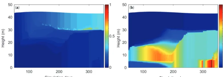
and the above diffusion algorithm is run once up the water column and once down the water column as a simple explicit method for capturing diffusion of mass to both the upper and lower layers. An example of the effect of hypolimnetic mix-ing on a hypothetical scalar concentration released from the sediment to the water column layers and accumulating in the hypolimnion is shown in Fig. 10.
2.7 Inflows and outflows
Aside from the surface fluxes of water described above, the water balance of a lake is controlled by inflows and out-flows. Inflows can be specified as local run-off from the sur-rounding (dry) lake domain (QRdescribed separately above; Eq. 8), rivers entering at the surface of the lake that will be buoyant or plunge depending on their momentum and density (Sect. 2.7.1), or submerged inflows (including groundwater) that enter at depth (Sect. 2.7.2). Four options for outflows are included in GLM. These include withdrawals from a spec-ified depth (Sect. 2.7.3), adaptive offtake (Sect. 2.7.4), ver-tical groundwater seepage (Sect. 2.7.5), and river outflow– overflow from the surface of the lake (Sect. 2.7.6). Any num-ber of lake inflows and outflows can be specified, and, ex-cept for the local run-off term, all are applied at a daily time step. Depending on the specific settings of each, these water fluxes can impact the volume of the individual layers,1Vi,
and the overall lake volume (Eq. 4). Inflows have a prescribed composition (temperature, salinity, and scalars), except local
run-off, which is assumed to be at air temperature with zero salinity.
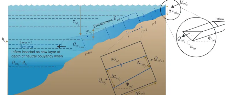
2.7.1 River inflows
As water from an inflowing river connects with a lake or reservoir environment, it will form a positively or negatively buoyant intrusion depending on the density of the incoming river water in the context of the water column stratification. As the inflow progresses towards insertion, it will entrain water at a rate depending on the turbulence created by the inflowing water mass (Fischer et al., 1979). For each con-figured inflow the entrainment coefficient,Einf, is computed based on the bottom drag being experienced by the inflowing water,CDinf, and the water stability using the approximation given in Imberger and Patterson (1981) as written in Ayala et al. (2014):
Einf=1.6C 3/2 Dinf
Riinf
, (60)
where the inflow Richardson number,Riinf, characterizes the stability of the water in the context of the inflow. Imberger and Patterson (1981) derived a simple estimate ofRiinfbased on the drag coefficient by assuming the velocity (and Froude number) is typically small and considering the channel ge-ometry, which is adapted in GLM as
Riinf=
CDinf 1+0.21p
CDinfsinαinf
sinαinftan8inf , (61)
a
c
e d
b
( ) Ellen Brook Nature Reserve
( ) Grosse Dhuenn
Height (m)
Height (m)
( ) Lake Kinneret
0 5 10 km
Ellen Brook Nature Reserve
Sparkling Lake
Lake Kinneret
Grosse Dhuenn
Woods Lake
( ) Woods Lake ( ) Sparkling Lake
Ice (m)
1.5 1.0 0.5
Height (m)
Height (m)
Height (m)
Height (m)
Height (m)
Simulation days Simulation days
Figure 9.A 2-year time series of the simulated temperature profiles for five example lakes(a–e)that range in size and hydrology. For more information about each lake and the simulation configuration, refer to the “Data availability” section (refer also to Figs. 2 and 5). Sparkling Lake(b)also indicates the simulated depth of ice on the RHS scale.
bottom roughness can be used to parameterize the character-istic rate of entrainment as it enters the waterbody.
On entry, the inflow algorithm captures two phases: first, the inflowing water crosses the layers of the lake until it reaches a level of neutral buoyancy, and second, it then un-dergoes insertion. In the first part of the algorithm, the daily inflow parcel is tracked down the lakebed and its mixing with layers is updated until it is deemed ready for insertion. The initial estimate of the intrusion thickness,1zinf0, is computed
as in Antenucci et al. (2005) and Ayala et al. (2014):
1zinf0= 2Riinf g0
inf
Q
inf0
tanαinf
2!1/5
, (62)
whereQinf0=finfQinfx is the inflow discharge entering the
domain based on the data provided as a boundary condition, Qinfx, andg
0
infis the reduced gravity of the inflow as it en-ters.
g0inf=g(ρinf−ρs) ρs