www.wind-energ-sci.net/1/205/2016/ doi:10.5194/wes-1-205-2016
© Author(s) 2016. CC Attribution 3.0 License.
Wind tunnel tests with combined pitch and free-floating
flap control: data-driven iterative feedforward
controller tuning
Sachin T. Navalkar1, Lars O. Bernhammer2, Jurij Sodja3, Edwin van Solingen1, Gijs A. M. van Kuik2, and Jan-Willem van Wingerden1
1Delft Center for Systems and Control, Faculty of Mechanical, Maritime and Materials Engineering,
Delft University of Technology, 2628 CD Delft, the Netherlands
2Wind Energy Group, Faculty of Aerospace Engineering, Delft University of Technology,
2629 HS Delft, the Netherlands
3Aerospace Structures and Computational Mechanics, Faculty of Aerospace Engineering,
Delft University of Technology, 2629 HS Delft, the Netherlands
Correspondence to:Sachin T. Navalkar ([email protected])
Received: 28 April 2016 – Published in Wind Energ. Sci. Discuss.: 17 May 2016 Revised: 31 August 2016 – Accepted: 8 September 2016 – Published: 26 October 2016
Abstract. Wind turbine load alleviation has traditionally been addressed in the literature using either full-span pitch control, which has limited bandwidth, or trailing-edge flap control, which typically shows low control authority due to actuation constraints. This paper combines both methods and demonstrates the feasibility and advantages of such a combined control strategy on a scaled prototype in a series of wind tunnel tests. The pitch-able blades of the test turbine are instrumented with free-floating flaps close to the tip, designed such that they aerodynamically magnify the low stroke of high-bandwidth actuators. The additional degree of freedom leads to aeroelastic coupling with the blade flexible modes. The inertia of the flaps was tuned such that instability occurs just beyond the operational envelope of the wind turbine; the system can however be stabilised using collocated closed-loop control. A feedforward controller is shown to be capable of significant reduction of the determin-istic loads of the turbine. Iterative feedforward tuning, in combination with a stabilising feedback controller, is used to optimise the controller online in an automated manner, to maximise load reduction. Since the system is non-linear, the controller gains vary with wind speed; this paper also shows that iterative feedforward tuning is capable of generating the optimal gain schedule online.
1 Introduction
The increasing size and flexibility of wind turbines demand that attention be devoted to the active and passive control of rotor loads in order to limit the costs related to both the construction as well as maintenance of the turbine blades and the support structure. The dominant dynamic loading of turbine components occurs at 1P (rotor speed) and its har-monics. One of the most interesting and readily accessible methods of blade load control are individual pitch control (IPC) (Bossanyi, 2003), whereby each blade is pitched along its longitudinal axis independently to counteract the
all the references mentioned, the target of IPC has been to reduce low-frequency loads, primarily around the 1P (rotor frequency). While IPC can, in this way, address a large part of load spectrum, the emphasis on low frequencies is also a product of the low bandwidth that can be achieved with the full-span pitch control, which involves actuation of the large torsional inertia of the blades around their axes. As expected, IPC also leads to a substantial increase in pitch activity.
In an effort to reduce pitch actuator duty, target higher fre-quencies in the load spectrum and address localised distur-bances in the wind loading, recent literature has explored the concept of the “smart” rotor (Lackner and Van Kuik, 2010), i.e. a rotor where the blades are instrumented with sensors and flow-modifying actuators at various radial locations. Re-views of such rotors (Barlas and Van Kuik, 2010; Bernham-mer et al., 2012) invariably conclude that trailing-edge flaps give the best control authority for load alleviation. The load alleviation potential has been demonstrated in simulations (Andersen et al., 2006; Bernhammer et al., 2016) and ex-perimentally in a wind tunnel (Van Wingerden et al., 2011). Further, field tests of this concept have also been conducted (Castaignet et al., 2013), although such a system is still not considered mature enough for incorporation in a commercial wind turbine. While these tests used conventional actuators, many references recommend the usage of smart actuators, such as piezoelectrics, in order to enhance bandwidth and achieve a high power-to-weight ratio. Such actuators unfor-tunately show low stroke and hence reduced control author-ity.
The concept of the free-floating flap (Heinze and Karpel, 2006) combines a trailing-edge flap that is free to rotate about its axis, with a small tab located on the flap that can be actu-ated at a high speed to dynamically change flap camber. This concept was developed specifically to take advantage of aero-dynamic levering to increase the low stroke of smart actua-tors. For a fixed wing instrumented with such a free-floating flap, it was experimentally shown (Bernhammer et al., 2013) that it is possible to achieve enhanced control authority. Fur-ther, this study also demonstrated that such a flap could be completely autonomous in terms of energy consumption and can be used as a lug-and-play device. This modularity shows promise for the construction and maintenance of a future smart blade. However, this concept has not yet been demon-strated experimentally on a wind turbine.
Numerical and experimental investigations of the free-floating flap concept (Heinze and Karpel, 2006; Bernham-mer et al., 2013) have shown that the additional degree of freedom adds a rigid-body mode to the system, the dynamics of which are strongly dependent on the total air speed at op-eration. Aeroelastic coupling of this mode with the flexible-blade mode induces flutter at low wind speeds, an instability that can lead to dangerously high vibrations and even struc-tural failure. However, it has also been shown in the refer-ences that closed-loop control of the tab can ensure safe oper-ation of a fixed wing, well into the unstable regime. A
pitch-able wind turbine blade instrumented with free-floating flaps thus poses several control challenges. Firstly, the nature of the flap implies that its dynamic response is not constant but varies strongly with the wind speed. Such a system cannot be described by a linear time-invariant (LTI) state-space re-alisation but can possibly be expressed as a linear-parameter-varying (LPV) system, where the time-linear-parameter-varying parameter de-pends on the wind speed. Further, the presence of a stabilis-ing closed-loop controller is mandatory. Finally, the uncer-tainties in flow and structure modelling imply that a robust controller may be unable to achieve the maximum possible load reductions. The advantage of using a data-driven con-trol strategy would be that input–output data could be used to (locally) optimise a simple user-defined criterion. Further, if such a strategy is used to tune a feedforward controller, then the optimised controller cannot, in the steady state, desta-bilise the plant, and in the best case, it may be able to achieve load reductions that may not be attainable by a conservative, globally robust controller.
Data-driven control of wind turbine loads has been demstrated experimentally in Navalkar et al. (2015), where line recursive system identification was combined with on-line controller synthesis for minimising the periodic turbine loads. However, such a controller would be required to retune itself at every instant the ambient wind conditions change. An alternative methodology for the data-driven alleviation of wind loads has been described in Navalkar and Van Winger-den (2015), and it employs the iterative feedback tuning (IFT) (Hjalmarsson, 2002) methodology to tune the gains of a fixed structure controller, hereby optimising a (convex) per-formance criterion. While IFT controllers have been used in the industry, they have typically been implemented to con-verge to linear-time-invariant controller structures (Gevers, 2002). The use of IFT for tuning the gains of time-varying controllers, as required for the current application, has been described in the literature (Navalkar and Van Wingerden, 2015) but not yet demonstrated in practice.
The contribution of this paper is thus threefold: firstly, scaled wind turbine blades instrumented with outboard free-floating flaps are designed and manufactured for wind tunnel testing. Secondly, the load alleviation potential of the free-floating flaps in combination with individual pitch control is demonstrated for the first time in an experimental sense. The load alleviation potential is investigated in both the sta-ble and unstasta-ble (post-flutter) modes of operation, and the importance of collocated control will be highlighted. Finally, the setup will serve as a test bench for a novel iterative feed-back tuning algorithm that automatically tunes a controller gain schedule for load alleviation in real-time variable wind speed operation. The innovations found in the paper are ex-plicitly stated below.
– This is the first experimental demonstration of
– This is the first experimental demonstration of free-floating flaps applied to rotating wind turbine blades. This is also the first time their potential has been demon-strated for load reduction in wind turbines experimen-tally. Further, this is the first time that free-floating flaps have been shown to induce flutter on wind turbine blades experimentally.
– This is the first experiment where IFT has been devised
and implemented for adaptively tuning the gain sched-ule on a non-linear (LPV) plant.
The remainder of the paper is organised as follows: Sect. 2 describes the design and manufacturing process for the wind turbine blades with free-floating flaps. Section 3 gives a brief description of the testing environment. The aeroelastic be-haviour of the blades is studied in Sect. 4. The control algo-rithm used for load alleviation is formulated in Sect. 5. The results of the testing are laid out in Sect. 6, and conclusions are drawn from these results in the final section.
2 Blade design and manufacturing
Since this paper reports on the first wind turbine implemen-tation of free-floating flaps, first, the design of the experi-mental setup is discussed, and details regarding the materials, method of manufacture and assembly are provided. Primar-ily, the destabilising effect of the free-floating flap is studied in detail, and the parameters are tuned such that the blade is close to its flutter point in order that maximal control author-ity is achieved.
The design of the blades formed the most important part of the design process of the scaled turbine, since it had to form a reasonable approximation of a full-scale wind turbine blade while adhering to the constraints set by the wind tun-nel capabilities. The primary scaling that was aimed to be achieved was maintaining the ratio of blade first eigenfre-quency to rotor speed (1P), as is done in Van Wingerden et al. (2011). This ratio is typically around 3.5 for the modern turbines (Bak, 2013).
2.1 Blade design
The overall aerodynamic and structural design of the blades follows the procedure described in Van Wingerden et al. (2011), since the blades were designed for similar wind tun-nel testing conditions. Aerodynamic and structural details of the blade design can be found in Hulskamp et al. (2011). However, as the wind tunnel experiments will also incorpo-rate blade pitch control, the torsional inertia of the blades was reduced by scaling down the root chord by 30 %. The root chord thus measures 200 mm, tapering to a tip chord value of 120 mm over a blade length of 750 mm, with a total blade twist of 12◦.
Out of structural considerations, it was deemed necessary to minimise the weight of the blades, while ensuring
ade-Figure 1.Blade CAD model.
Figure 2.Photograph of blade.
quate structural integrity to withstand the centrifugal and out-of-plane loading that the blade will be subject to during op-eration. An accurate aerodynamic shape of the blade was en-sured by 3-D printing the blade and then further reinforced with unidirectional carbon fibre spar caps, as shown in Fig. 1. Small wind turbine blades have previously been manufac-tured in this manner by the University of Stuttgart (Bauer et al., 2014), and a comparison of different additive manu-facturing techniques can be found in Karutz (2015). These references specifically investigate 3-D printing of blades in a set of sections that are bonded together. In order to avoid solid plastic–plastic joints, it was decided that the blades in the current case would be printed in one piece.
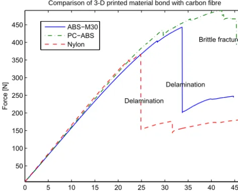
Three different materials (ABS M30, PC-ABS and nylon) that can be used for 3-D printing were evaluated regarding their ability to bond with carbon fibre. For each material, a
rectangular sample 200 mm×30 mm in size and 3 mm thick
0 5 10 15 20 25 30 35 40 45 50
100 150 200 250 300 350 400 450
Deformation [%]
Force [N]
Comparison of 3-D printed material bond with carbon fibre
Delamination
Delamination
Brittle fracture ABS−M30
PC−ABS Nylon
Figure 3. Structural behaviour of the bond between 3-D printed
substrate and carbon fibre spar.
Figure 4.The grey rectangle on the top and the two black
rectan-gles below it are the 3-D printed samples post fracture, placed on a sandstone-coloured desktop that forms the background. Top: ABS M30; middle: PC-ABS; bottom: nylon.
apart. The results of the test can be seen in Figs. 3 and 4. In Fig. 3, the behaviour to failure in bending can be observed. For small loads, the response is linear. At higher loads, small kinks can be observed in each of the curves; these physically represent the snapping of individual carbon fibres in com-pression. Finally, there is a large drop in strength when de-lamination occurs in the materials ABS M30 and nylon. For the material PC-ABS, brittle fracture occurs before delami-nation; thus the bond between this material and the carbon fibre spar is the best for this material. Further, it also holds its strength over a larger range of deformation than the other materials. Since PC-ABS also shows good mechanical work-ability, the choice was made to 3-D print the scaled blade using this material.
The blade was printed as a 3 mm thick shell, with an in-ternal spar structure, using stereolithography techniques. In
0 5 10 15 20 25 30
0 5 10 15 20 25 30 35 40 45 50
Tip deflection [mm]
Tip load [N]
Blade stiffness: simulation vs. measurement
Measured, w/o carbon fibre Measured, with carbon fibre Calculated, w/o carbon fibre Calculate, with carbon fibre
Figure 5.Calculated stiffness characteristics compared with
mea-sured stiffness characteristics.
order to add structural stiffness to the blades, a spanwise slot was engraved at the spar cap location on both the top and bottom of the blade. This slot was filled with a 0.14 mm thick layer of unidirectional carbon fibre tow impregnated with epoxy resin. The slot was then aerodynamically faired using crushed glass fibre epoxy filler, which was then sanded down for a smooth finish. A computer-aided design (CAD) model of the blade and a photograph of the finished blade are shown in Figs. 1 and 2. The CAD software Solidworks was used for designing the blade, with the blade material consid-ered to be homogeneous and isotropic. The metal connection to the hub and the carbon fibre are modelled to be bonded to the blade ideally such that delamination is not possible. An ultimate loading case is simulated for a wind speed of 10 m s−1, rotor speed of 400 rpm and a thrust coefficient of 1. For this extreme case, the stresses in the plastic material are calculated to be less than the flexural strength of the ma-terial by a factor of safety of 1.3.
The designed static force-deflection curve, compared with the measured structural behaviour, is seen in Fig. 5. It is in-teresting to note that the predicted stiffening effect of the car-bon fibre layer is nearly identical. The tip deflection was cal-culated to be 17.2 % lower with carbon fibre spars, while it was measured to be 16.6 % lower after stiffening. A flexible mode analysis of the blade yields its first natural frequency as 16.43 Hz.
Figure 6. Flap cross section: trim tabs replaced by chordwise piezobenders.
2.2 Free-floating flap (FFF) design
The CAD design of the free-floating flaps is depicted in Fig. 6. The leading edge is a continuation of the inboard por-tion of the blade, including the slot meant for carbon fibre stiffening. The hinge axis of the flap is mounted using bear-ings on an aluminium bracket just behind the spar; apart from the negligible bearing friction, it is entirely free to rotate. A T section is connected to this axle, such that its interference with the mounting bracket provides limit stops for the rota-tion of the flap. The flap can hereby rotate freely through a
maximum upward and downward deflection angle of 30◦.
A metal plate (spring steel) 0.2 mm thick is sandwiched between the axle and the T section. Two piezobenders (Macrofibre composite, type M8557-P1) are affixed rigidly to the top and the bottom of this metal plate. The benders are electrically connected together in an antiparallel manner such that their piezoelectric effects reinforce each other and they produce the same magnitude but an opposite direction
of strain in the substrate. A maximum voltage of±500 V can
be applied to the benders in order to emulate the behaviour of the trim tab from Heinze and Karpel (2006) and Bernhammer et al. (2013). Finally, an appropriate aerodynamic shape of the flap was achieved by embedding the instrumented metal plate into a highly compliant foam which was shaped accord-ing to the aerofoil geometry. The entire flap, from the angle-limiting T section to the foam spacers, is covered with a fair-ing shroud. A contactless angle encoder is embedded into the tip section, which provides feedback on the flap angular po-sition.
This configuration causes a step change in the chordwise profile just aft of the spar, which produces undesirable aero-dynamic behaviour, which is a well-known trade-off for the increase in the deformability of the trailing edge. In this ex-periment, to achieve a proof of concept for free-floating flaps, aerodynamic accuracy is sacrificed for control authority in the design of the flap.
Figure 7.Photograph of flap.
3 Aeroelastic blade analysis
While in the previous section it was ensured that the be-haviour of the blade under the ultimate static structural load was acceptable, an aeroelastic analysis is required to deter-mine the change in its structural response with increasing wind speed. The rigid-body mode of the free-floating flap is expected to couple with the first flexible mode of the system, giving rise to a low wind speed form of flutter.
In order to analyse the aeroelastic behaviour of the blade instrumented with a free-floating flap, the blade is modelled in MSC Nastran as a cantilever beam of non-uniform cross section (CBAR elements). The various cross sections of the modelled beam were taken at 10 equidistant spanwise sta-tions along the blade. Each element is rigidly connected to a flat-plate aerodynamic panel of the corresponding chord-wise length. The flap is modelled in a similar manner. First, a structural modal analysis of the blade is carried out, at zero wind speed. The calculated modes of the blade are given in Table 1. The corresponding modal frequencies predicted by Solidworks are as follows:
– first flapwise frequency: 18.97 Hz (Solidworks),
19.44 Hz (Nastran)
– first edgewise frequency: 78.37 Hz (Solidworks),
76.67 Hz (Nastran)
– second flapwise frequency: 84.8 Hz (Solidworks),
87.88 Hz (Nastran).
Table 1.Structural modes of the blade at zero total air speed.
Mode description Modal frequency Mode description Modal frequency
Rigid-body flap mode 0 Hz first flapwise mode 19.44 Hz First lead–lag mode 76.67 Hz second flapwise mode 87.88 Hz Third flapwise mode 223.9 Hz second lead–lag mode 291.3 Hz First Torsional mode 361.6 Hz fourth flapwise mode 449.6 Hz
data-driven controller that tunes itself in accordance with the true system parameters.
It is most interesting to note that the lowest flexible mode is the flapwise mode, with a modal frequency of 19.44 Hz. This is the mode most likely to couple unstably with the rigid body flap mode. The blade is significantly stiffer in both the lead–lag and torsional directions; these modes are hence un-affected by aerodynamic coupling. An actual turbine blade (Bak, 2013) is relatively softer in these directions; however, even for such a blade, the flapwise mode is the most rele-vant one for load analysis and also possesses the lowest fre-quency. The current scaled blade design, with high lead–lag and torsional stiffness, allows us to study the low-speed flut-ter phenomenon with limited complexity.
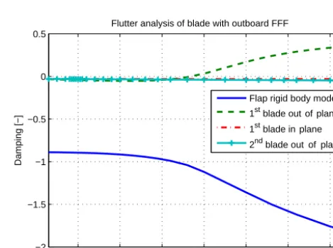
The low-speed flutter phenomenon, as predicted by Nas-tran, can be seen in Figs. 8 and 9. Here, the abscissae cor-respond to total air speed, which is defined as the resul-tant of the inflow wind speed and turbine rotational speed at the blade tip. It should be noted that the speed regula-tion trajectory of the wind turbine is linear, such that ro-tor speed increases linearly with wind speed at the rate of 51.1 rpm (m s−1)−1.
For the purpose of aeroelastic analysis, the blade has been considered to be held stationary, with inflow wind speed equal to the total air speed defined above. This assumption is not strictly valid, since the incident wind speed is lower at the inboard sections of the blade. However, since these sec-tions undergo lower structural deformasec-tions, it is expected that the impact on the aeroelastic behaviour of the blade is also lower. Further, the blade is twisted such that the an-gle of attack along the span remains more or less constant. Since the blade is non-rotating and subject to constant wind flow, the aerodynamic panels attached to each section main-tain a constant angle along the blade span. With these simpli-fying assumptions, a first-order approximation of the flutter behaviour of the turbine blade is synthesised.
It can be directly observed that the frequency of the rigid body flap mode rises linearly with total air speed. Due to coupling of this mode with the first blade flexible mode, the blade mode becomes unstable at the onset of flutter. For the given physical configuration of the blade, flutter occurs at a total air speed of 36 m s−1, which corresponds to a turbine
10 20 30 40 50 60 70
0 10 20 30 40 50 60 70 80 90
Wind speed [m s ]
Frequency [Hz]
Flutter analysis of blade with outboard FFF
Flap rigid body mode
1 blade out of planest
1 blade in planest
2 blade out of planend
-1
Figure 8. Variation in modal frequency with total incident air
speed.
10 20 30 40 50 60 70
−2 −1.5 −1 −0.5 0 0.5
Wind speed [m s ]
Damping [−]
Flutter analysis of blade with outboard FFF
Flap rigid body mode
1 blade out of planest
1 blade in planest
2 blade out of planend
-1
Figure 9.Variation in modal damping with total incident air speed.
rotor speed of 340 rpm, and thus at a speed beyond the
de-signed operational speed of the wind turbine (230 rpm).1
1In principle, a higher (pre-flutter) rotor operational speed of up
5 10 15 20 25 30 35 40 45 −0.1
−0.05 0 0.05 0.1 0.15 0.2
Variation of flutter speed with flap inertia
Total incident air speed
Modal damping [−]
67.5 g cm2
112.5 g cm2
270 g cm2
450 g cm2
607.5 g cm2
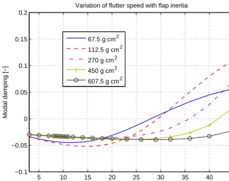
Figure 10.Variation of flutter speed with flap inertia.
The aeroelastic analysis served as a guideline for design-ing the kinematic parameters of the free-floatdesign-ing flap. A sensitivity analysis showed that the flutter speed depends strongly on the inertia of the flaps about the hinge axis. As seen in Fig. 10, an increase in flap inertia increases the flut-ter speed. Since an increase in flutflut-ter speed is also associated with a decrease in control authority, the flap inertia is chosen such that flutter occurs at a speed just beyond the operational regime of the wind turbine. The flap inertia is chosen to be 270 g cm−2, so that the flutter speed is 36 m s−1, as described before.
This aeroelastic analysis also served as a guideline for the design of the blades and for identifying the range of opera-tion permissible in the experiments described in the sequel. Experimentally, it was observed that the onset of flutter oc-curred at 315 rpm. However, since this mode involves ex-ponentially diverging vibrations in the blades, which cannot be physically limited, open-loop experiments in this unstable regime were not conducted out of safety considerations.
4 Testing environment
The blades designed and analysed as above were mounted on the test turbine setup used previously in Navalkar et al. (2015). As described in this reference, the blades are con-nected to the hub through pitch servomotors.
The hub is mounted on a shaft supported by two main bearings located in the nacelle. The electrical connections of the hub are transferred to the stationary part of the wind turbine via slip rings, rated at 500 V, which is also the maxi-mum voltage that can be fed to the piezobenders located out-board on the blades. Further, the shaft is instrumented with
current tower design yields a very lightly damped tower torsional mode at 280 rpm, which it is deemed necessary to avoid out of prac-tical considerations.
Figure 11.Photograph of the assembled turbine with pitch and flap
control.
a torque transducer and speed encoder and connected me-chanically to the generator. The turbine is direct-drive; the rotor speed is the same as the generator speed. The generator is in turn connected electrically in series with an adjustable dump load amenable to resistance control. Thus, in principle this setup can also provide torque control. However, in this series of tests, the resistance of the dump load is kept con-stant. This implies that the wind turbine is in constant torque operation, and its rotor speed rises linearly with the incom-ing wind speed. This form of control deviates from classical variable-speed, variable-pitch turbine control, which utilises collective pitch to ensure constant speed regulation above rated wind speed. However, the variable-speed constant-load operation of the scaled turbine serves three purposes: over-speed behaviour can be investigated, which may induce flut-ter, below-rated turbine behaviour can be emulated, and the use of adaptive control can be evaluated in terms of its ability to retune itself to adapt to changed operating conditions.
The nacelle is connected rigidly to the top of a tower, mounted on bearings on its base. The tower (and hence the entire wind turbine) can yaw freely around its base. For this set of experiments, the tower is kept fixed such that the plane of the rotor is always perpendicular to the incoming wind speed.
The entire assembly is mounted inside the Open Jet Facil-ity of the Delft UniversFacil-ity of Technology, which is an open jet wind tunnel of 6 m test cross section and 2.85 m equivalent open jet diameter. A photograph of the turbine can be seen in Fig. 11. While wind speeds up to 35 m s−1can be achieved in this wind tunnel, the operation of the wind turbine under the current settings requires no more than 6 m s−1, with a rated wind speed of 4.5 m s−1(and thus a tip speed ratio of 5.35).
There are two primary sensing elements: the load sensors at the blade roots and the free-floating flap angle sensors. Fur-ther, there are two primary actuators: the piezobenders on the flaps and the pitch motors. The objective of the experiments is to use these sensing and actuating elements to achieve load control of the scaled wind turbine.
5 Iterative feedforward tuning for combined pitch and flap control
For a wind turbine in the field, the blade loads arise mainly out of wind shear, tower shadow, turbulence and its rotational sampling. As such, the blade load spectrum for a typical tur-bine shows dominant peaks at the rotor speed (1P) and its harmonics: for a two-bladed turbine at 2P, 4P, and so on, while for a three-bladed machine at 3P, 6P, etc. The pres-ence of turbulpres-ence broadens these peaks and adds energy in the high-frequency region of the spectrum.
In the wind tunnel environment, the levels of turbulence are low. The main cause of the blade loads is the tower pas-sage, which leads to sharp peaks at 1P and its harmonics. The objective of the experiments is to demonstrate that these peaks can be attenuated by pitch and flap control, which by extension implies that a significant portion of the load spec-trum of an in-field turbine can be addressed by these actua-tion and control methods.
For achieving load control, IFT of the pitch and flap con-trollers will be implemented. This technique specifically tar-gets deterministic disturbances, as seen in the blade load spectrum of the turbine, with minimal control action. As long as there exists a nominally stabilising controller in the loop to avoid the unstable flutter region, the controllers tuned us-ing IFT will not render the plant unstable. Further, IFT en-sures that data-driven tuning of the controllers makes them converge to an optimal control action over a number of iter-ations.
It should be noted that this optimality refers to the local optimum of the user-defined cost criterion and is unrelated to global controller optimality. There are, at present, no global optimality proofs for IFT. Indeed, if a feedback controller is tuned using IFT for a poorly designed performance criterion, it may yield an unstable closed loop. However, since this pa-per considers IFT for feedforward control, this issue is not relevant. Further, if the step size in the gradient descent algo-rithms is too large, the parameter tuning process may become unstable. These issues have been dealt with by Hjalmarsson (2002).
The optimal controller parameters depend strongly on the incoming wind speed and hence demand an LPV controller. LPV controller tuning using IFT has been explored and shown to work in the simulation environment (Navalkar and Van Wingerden, 2015). However, the computational burden and number of experiments required for tuning imply that this methodology is required to be modified to meet the
demands of real-time control in the wind tunnel. Hence, a quasi-LPV approach will be followed in this section. Ac-cordingly, while the plant remains LPV at all times, when the wind speed varies slowly in the wind tunnel and the plant is approximated as LTI for the duration of each set of IFT experiments.
As a consequence of this assumption of constant dynam-ics, IFT tunes controller parameters that are optimal only for one specific operating point, while being suboptimal for the rest of the operating range. It is for this reason that the or-dinary IFT process has to be repeated for different constant wind speeds, or an IFT gain schedule has to be generated for a varying wind speed.
Firstly, the notation for this section will be introduced, then the three IFT experiments will be described and, finally, the method for creating a gain schedule for controller wind speed adaptivity is described.
5.1 Preliminaries and notation
An LPV formulation is set up for describing the wind tur-bine system, either in an open loop or in a closed loop with a nominally stabilising controller that allows the system to be operated in a post-flutter regime:
xk+1=Akxk+Bkuk, (1)
yk=Ckxk+Dkuk+vk. (2)
In these equations,xk∈Rnx is the state vector of unknown size,uk∈R4is the control inputs, including the two pitch
signals and the two flap signals, and yk∈R2 is the blade
load signals as measured by the sensors located at the roots of the two blades. The signalvk∈R2is the external forcing signal, produced in this case by tower passage; it is a super-position of a periodic signal with zero mean white noise. The state-space matricesAk,Bk,Ck andDk are considered un-known and have the appropriate dimensions. Although the system matrices are unknown, they are assumed to admit a specific LPV structure, as per Van Wingerden (2008). These matrices, as well as the disturbancevk, are considered to be affine functions of the ambient wind speed,Vk∈R:
Ak=A[0]+VkA[1], (3)
and similarly for the other matrices. Here,A[0]andA[1]
sig-nify the unknown components ofAk, one of which remains
constant over time and one of which varies linearly with the wind speed, respectively. As per Van Wingerden (2008), there should be one more term that varies withVk2, but the influence of this term is limited and it is ignored in this pa-per.
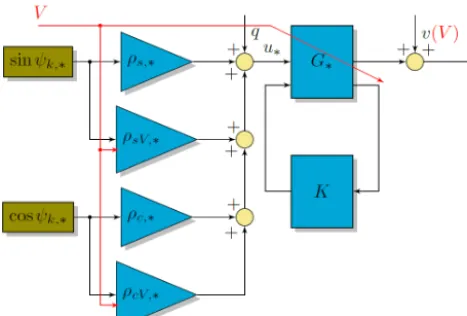
Figure 12.IFT implementation: wind turbine load control. Asterisk stands for IPC or individual flap control (IFC).
angle in the above-rated region and the generator speed in the below-rated region to approximate the value of ambient wind speed; in the current experiments the latter approach is used. In the theoretical framework, it is hence assumed that the controller possesses perfect knowledge of the wind speed.
The feedforward disturbance attenuating controller to be designed is considered to be a full LPV controller parame-terised as follows:
ξk+1=Ac,k(ρ)ξk+Bc,k(ρ)rk, (4)
uk=Cc,k(ρ)ξk+Dc,k(ρ)rk−qk. (5)
Here, the controller is considered to be a fixed structure troller, such as a proportional integral derivative (PID) con-troller, with stateξ∈Rnc of fixed dimension. The reference signal for this controller is taken to be a set of azimuth-locked basis functions, as in Navalkar and Van Wingerden (2015), thereby rendering this method a form of adaptive cyclic pitch and flap control. This form of open-loop control is depicted in the block diagram in Fig. 12. For the pitch controller, these are sinusoidal functions of frequency 1P, while for the flap controller, these are sinusoidal functions of frequency 2P. Thus, the pitch and the flap control are both decoupled in the frequency domain and are expected to strictly attenuate loads at their respective frequencies, in order to mitigate the maximum amount of disturbance with a minimum of control effort. Thus, with two sinusoidal basis functions for each fre-quency 1P and 2P, the reference signal isrk∈R4. The term
qk refers to an auxiliary input that will be used in the IFT
experiments described in the next subsection.
The objective of IFT is to minimise the loads as measured by the load sensors; so the cost criterion is
J = 1
2N(y
Ty), (6)
whereN is a sufficiently long prediction horizon. For
atten-uating periodic loads,N is taken to be a multiple of the fun-damental period of these loads. The termy∈R2Nis the load
signal stacked over this horizon:y= [y1T, y2T, . . ., yTN]T. The other signals are stacked in a similar manner. The key ele-ment of the IFT methodology is the optimisation of the sys-tem performance with the help of an experimentally derived performance gradient with respect to the controller parame-ters. This performance gradient is given by
∂J ∂ρ =
1
N ∂yT
∂ρ y. (7)
Since the gradient contains stacked signals, it is more con-venient to cast the system equations into a lifted format. Thus, for instance, the lifted system matrix for the wind tur-bine plant is given by the Toeplitz-like matrixT∈R2N×4N
as
T=T(Ak,Bk,Ck,Dk)= (8)
D1 0 · · · 0
C2B1 D2 · · · 0
C3A2B1 C3B2 · · · 0
C4A3A2B1 C4A3B2 · · · 0 ..
. ... . .. ...
CNAN−1. . .B1 CNAN−1. . .B2 · · · DN
.
Like this lifted plant matrixT, a similar lifted matrixTccan be constructed for the controller. It can be observed that the
system matrices are functions of the wind speedVk, which
is approximated to be constant for each set of IFT experi-ments but changes over the course of different sets of IFT experiments (or IFT iterations). As such, for the case where the wind speed is held constant atV∗for a set of IFT
exper-iments, the system matrices of the plant and the controller areT(V∗) andTc(V∗), respectively. The LTI IFT set of
ex-periments that yield the controller gradient for the fixed wind speedV∗are described next.
5.2 IFT experiments
In traditional IFT (Hjalmarsson, 2002), designed for LTI sys-tems, the controller parameters can be iteratively optimised by repeatedly conducting a set of three experiments for each controller parameter. If the wind speed is considered to be constant over this set of experiments, the wind turbine plant reduces to an LTI system, and the same approach can be fol-lowed for optimising controller parameters for that specific wind speed. This section recapitulates the IFT methodology from this perspective.
In the first IFT experiment, the auxiliary signal is set to zero (qI=0). It is assumed that, over the set of these
ex-periments, the wind speed is constant at a value ofV∗.
Ac-cordingly, the output data collected are related to the system matrices as
Considering Eq. (7), in order to find the performance gra-dient, it is necessary to determine the gradient of the out-put with respect to the parameters, ∂y∂ρ. As such, the equation above is differentiated with respect to each controller param-eterρjρ,jρ=1, . . ., nρ, wherenρis the number of controller parameters. This results in the following equality:
∂yI ∂ρjρ
=T(V∗)
∂Tc(V∗)
∂ρjρ
r. (10)
It should be noted that in the above equation, the only un-known on the right-hand side is the system matrix of the plant,T(V∗). In order to estimate its filtering effect, the
sec-ond experiment uses the following auxiliary input:
qII=
∂Tc(V∗)
∂ρjρ
r. (11)
Thus, the output in the second experiment becomes
yII=(T(V∗)−T(V∗)
∂Tc(V∗)
∂ρjρ
)r+vII(V∗). (12)
The required output gradient ∂ρ∂yI
jρ is now given by
∂yI
∂ρjρ
=yI−yII+vII(V∗)−vI(V∗). (13)
Since the disturbance signalvis a superposition of a periodic
signal and random noise and the stacking lengthNis a
mul-tiple of period of the noise, the termvII(V∗)−vI(V∗) does not
contain a periodic component and is purely zero mean white noise. The output gradient below is ergodically unbiased:
∂yˆI ∂ρjρ
=yI−yII. (14)
However, the performance gradient cannot in this case be constructed simply as
∂J ∂ρjρ
V=V
∗ = 1
N(yI−yII) Ty
I. (15)
This is because the noise in the estimate of the output gra-dient ∂ρ∂yI
jρ is correlated with the disturbance components in
yI, and the performance gradient estimate would hence be
biased. So, a third experiment, replicating the determinis-tic conditions of the first experiment, is required to be con-ducted, in order to obtain the statistically uncorrelated output
yIII. Finally, the performance gradient is given by
∂J ∂ρjρ
V=V∗ = 1
N(yI−yII) Ty
III. (16)
With this performance gradient estimated from data, an optimisation method, such as a steepest-descent method, can
now be employed to obtain the optimal value of the controller parameter. It is to be noted, however, that the controller pa-rameter derived in such a manner is optimal only for the op-erating wind speed. The iterations for achieving such a con-ditionally optimal controller parameter can be denoted by
ρji+1
ρ (V∗)=ρ
i
jρ(V∗)−γ
iR−1 ∂J ∂ρjρ
V=V∗
. (17)
Here, the termγis an (iteration-dependent) scalar step size that can be tuned for achieving the desired convergence rate. It should be noted that a step size that is too large may lead
to non-convergence. The termRrepresents a positive
defi-nite matrix, which is identity for the steepest-descent method but can be the Hessian matrix or an estimate of the Hessian matrix with respect to the controller parameter for increasing the rate of convergence.
With this method, the optimal controller parameters for a specific wind speed can be iterated to. The next section de-tails the synthesis of a gain schedule for adapting the param-eters for the case with slowly varying wind speed.
5.3 Data-driven gain schedule synthesis
The previous section details the manner in which, for a con-stant wind speed, an updated estimate of the ideal controller parameters for that wind speed can be obtained. In this sec-tion, it is assumed that, in each iterationi, the ideal
param-eters vary as an affine function of the wind speedVi in the
following manner:
ρj∗
ρ(V
i)=ρ[0],∗
jρ +V iρ[1],∗
jρ . (18)
While the above equation indicates a linear relationship
be-tween the optimal parameter and the scheduling variableV,
this may not in practice always be the case. However, the same equation can also be extended to an arbitrarily high degree of complexity, using either polynomial or any other suitable basis functions. The choice of the number of func-tions depends upon the non-linearity of the scheduling, and on the signal-to-noise ratio achieved by the sensors, and may in practice be difficult to estimate a priori.
The objective of IFT is then to iterate to the optimal values ofρj[0]
ρ andρ
[1]
jρ based on the data inferred from the
experi-ments described in the previous section. In the simple case of affine scheduling dependence described above, this can be achieved by recursive least squares estimation of the gain schedule. Thus, at every iteration that a pairρji+1
ρ andV
i+1
is obtained from Eq. (17), recursive linear regression is used to update the gain schedule.
Magnitude (dB)
-60 -40 -20 0 20
340 rpm: unstable 300 rpm 230 rpm 200 rpm
10-1 100 101 102 103
Phase (deg)
-180 -90 0 90 180
Transfer from tab deflection to blade root load
Frequency (rad s )-1
Figure 13.Transfer from piezobender actuators to blade root loads
at different wind speeds.
6 Results
To recapitulate, the objective of the wind tunnel experiments was to achieve blade load control for the scaled wind turbine, using full-span pitch actuation and free-floating flap control, with iterative forward tuning for optimal performance of the load controller. It should be noted that since experiments are conducted under constant load operation, the rotor speed varies linearly with wind speed. Thus, a rated wind speed of 4.5 m s−1corresponds to a rotor speed of 230 rpm. The flutter speed of 6 m s−1(total air speed 34 m s−1) corresponds to a rotor speed of 315 rpm. In this section, operating conditions will be designated by the operating rotor speed.
6.1 System identification and stabilising controller
Initially, the response of the wind turbine blade to flap actua-tion is studied and compared with the simulaactua-tions. Open-loop identification experiments are conducted in the pre-flutter regime (200–300 rpm), with a zero-mean white noise
(max-imally ±500 V) imposed on the piezobenders.
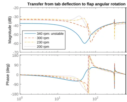
Predictor-based subspace identification (PBSID) (Van der Veen et al., 2013) is performed using the acquired data to obtain the transfer function between the tab actuation and the flap angle and blade root load measurements. The transfer functions are depicted in Figs. 13 and 14.
It can be observed that significant phase loss occurs in the transfer from the actuator to the blade root loads. This im-plies that stabilising the system using the measurements from the root loads poses a control challenge, and it may prove difficult in the case of uncertain systems to guarantee robust stability in the unstable post-flutter region. Further, it also motivates the use of local load sensors to enhance load atten-uation capabilities. On the other hand, the phase loss in the
Magnitude (dB)
-70 -60 -50 -40 -30 -20
340 rpm: unstable 300 rpm 230 rpm 200 rpm
100 101 102 103
Phase (deg)
-180 -90 0 90 180
Transfer from tab deflection to flap angular rotation
Frequency (rad s )-1
Figure 14.Transfer from piezobender actuators to free floating flap
angle at different wind speeds.
transfer between the actuator and the flap angle measurement is minimal. This collocated sensor is hence ideal for system stabilisation in the post-flutter region. A simple classically tuned controller is used for stabilisation; it is not designed for load reduction and is hence not optimal. It is described in continuous time as follows:
K= 0.0001 | {z } Static gain
s/0.001+1
s/10+1
| {z }
High pass
(19)
s2+0.001s×50/2π+(50/2π)2
s2+0.1s×50/2π+(50/2π)2
| {z }
Notch for 50 Hz electrical back-coupling artefact 1 2π s/100+1
| {z }
Low pass .
Number of iterations [1 iteration = 8 s] 5 10 15 20 25 30
Controller gains [-]
-4 -3 -2 -1 0 1 2 3
4 IFT tuning of pitch and flap controller gains
Blade 1, ρs,IPC
Blade 2, ρs,IPC
Blade 1, ρc,IPC
Blade 2, ρc,IPC
Blade 1, ρs,IFC
Blade 2, ρs,IFC
Blade 1, ρc,IFC
Blade 2, ρc,IFC
Figure 15.Convergence of controller gains over iterations.
6.2 Optimal IFT for constant wind speeds: pre-flutter
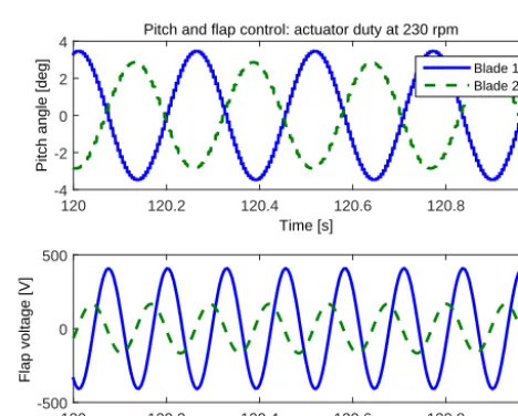
The next step was to study the effect of the IFT load con-trollers for combined pitch and flap control. The block dia-gram for the load controllers is shown in Fig. 12. Accord-ingly, the pitch and flap actuation signals were combinations of 1P and 2P sinusoidal basis functions, respectively. The basis functions are scheduled on the azimuth and are hence phase-locked. IFT was used to train the amplitudes of these basis functions; thus, with two basis functions for each fre-quency and each blade, for both pitch and flap control, a total of eight gains were required to be tuned.
The IFT process was first studied for a constant oper-ational speed. Selected results, at an operoper-ational speed of 230 rpm, are presented here, although similar results were also observed throughout the operational range. The con-vergence of the controller gains and the IFT cost criterion can be seen in Figs. 15 and 16. It can be seen that, within 10 min, the controller gains converge to their optimal values. The performance of the controller after convergence can be visualised in Figs. 17 and 18. The figures show that the ac-tuation demanded, both pitch and flap, is purely sinusoidal, as constrained by the respective basis functions. Further, the load components in the blade load spectrum at the frequen-cies 1P and 2P are almost entirely eliminated by the pitch and flap action, respectively. Thus, IFT is successful in tuning the controllers as required.
One final point of note is that the converged gains for the two blades are not exactly antisymmetric; this is especially pronounced for the flap actuation. The primary reason for this is a difference in the manufacture of the two blades. Specifi-cally for the flap dynamics, for the scaled blade, a difference in the order of a few grammes in its weight distribution can strongly alter system dynamics and even prepone the onset of flutter.
Commercially manufactured blades are ideally expected to be identical; they would require antisymmetric pitch action
0 50 100 150 200 250
0 0.01 0.02 0.03 0.04 0.05 0.06
Time [s]
Performance criterion y
Ty/N
Minimisation of IFT performance criterion
Figure 16.Minimisation of IFT cost criterion over iterations.
Time [s]
120 120.2 120.4 120.6 120.8 121
Pitch angle [deg]
-4 -2 0 2
4 Pitch and flap control: actuator duty at 230 rpm
Blade 1 Blade 2
Time [s]
120 120.2 120.4 120.6 120.8 121
Flap voltage [V]
-500 0 500
Figure 17. Actuator duty cycles of optimised controller
(pre-flutter).
and identical flap action for load attenuation, as produced by a conventional IPC controller (Bossanyi, 2003). Such a con-troller does not achieve optimal load reduction in the case of there being discrepancies in blade manufacture or aging. The IFT controller designed above is thus shown capable of accounting for blade asymmetry and adjusting control action for maximising load reduction.
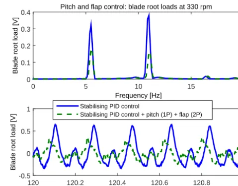
6.3 Optimal IFT for constant wind speeds: post-flutter
Frequency [Hz]
0 5 10 15 20
Blade root load [V]
0 0.1 0.2
0.3 Pitch and flap control: blade root loads at 230 rpm
Time [s]
120 120.2 120.4 120.6 120.8 121
Blade root load [V]
-0.4 -0.2 0 0.2 0.4
No control Pitch (1P) + Flap (2P)
Figure 18.Load reductions achieved by optimised controller
(pre-flutter).
Time [s]
120 120.2 120.4 120.6 120.8 121
Pitch angle [deg]
-2 -1 0 1
2 Pitch and flap control: actuator duty at 330 rpm
Time [s]
120 120.2 120.4 120.6 120.8 121
Flap voltage [V]
-500 0 500
Blade 1 Blade 2
Figure 19. Actuator duty cycles of optimised controller
(post-flutter).
tune the feedforward load-reducing pitch and flap controller gains in a manner similar to the previous experiments; how-ever, in this case the underlying plant is the stabilised post-flutter wind turbine in a closed loop with the PID controller. From Figs. 19 and 20, it can be seen that the optimised IFT controller gains are still able to achieve load reduction even in this highly challenging unstable operational regime. Fig-ure 19 shows that the pitch controller no longer issues an-tisymmetric commands; a traditional IPC controller is no longer adequate in this region. Further, the flap command has
already reached its maximum limits of±500 V.
Frequency [Hz]
0 5 10 15 20
Blade root load [V]
0 0.1 0.2 0.3
0.4 Pitch and flap control: blade root loads at 330 rpm
Time [s]
120 120.2 120.4 120.6 120.8 121
Blade root load [V]
-0.5 0 0.5
1 Stabilising PID control
Stabilising PID control + pitch (1P) + flap (2P)
Figure 20.Load reductions achieved by optimised controller
(post-flutter).
0 50 100 150 200 250 300 350
185 190 195 200 205 210 215 220 225 230 235
Time [s]
Rotor speed [rpm]
Varying wind speed/rotor speed profile
Figure 21. Varying operational speed for optimisation of gain
schedule.
6.4 Optimal IFT gain schedule for varying wind speeds
Time [s]
50 100 150 200 250 300 350
Gain schedule coefficients [-]
-5 0 5
10 Gain schedule intercepts, ρ
[0]
Blade 1, ρs,IPC
Blade 2, ρs,IPC
Blade 1, ρc,IPC
Blade 2, ρc,IPC
Blade 1, ρs,IFC
Blade 2, ρs,IFC
Blade 1, ρc,IFC
Blade 2, ρc,IFC
Figure 22. Optimisation of gain schedule intercepts for varying
wind speed conditions.
Time [s]
50 100 150 200 250 300 350
Gain schedule coefficients [-]
-3 -2.5 -2 -1.5 -1 -0.5 0 0.5
1 Gain schedule slopes, ρ
[1]
Blade 1, ρs,IPC
Blade 2, ρs,IPC
Blade 1, ρc,IPC
Blade 2, ρc,IPC
Blade 1, ρs,IFC
Blade 2, ρs,IFC
Blade 1, ρc,IFC
Blade 2, ρc,IFC
Figure 23.Optimisation of gain schedule slopes for varying wind
speed conditions.
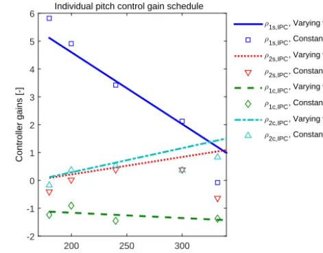
scheduling parameter. However, as the wind speed changes beyond this point in time, the gain schedule rapidly con-verges to an optimum. The gain schedule finally achieved is compared with the optimal controller gains obtained from the previous set of experiments in Figs. 24 and 25. It can be seen that for the pitch controller, the linear gain schedule obtained is a good fit to the optimal values obtained at constant wind speed. On the other hand, the flap controller optimal gains show a non-linear variation with wind speed, and the linear gain schedule obtained achieves a reduced goodness of fit.
Thus, the combined pitch and flap controller has been shown to be able to reduce blade loads both in pre- and post-flutter conditions. Further, an optimal gain schedule for these controllers is automatically tuned online using IFT in varying wind conditions.
Rotor speed [rpm]
200 250 300
Controller gains [-]
-2 -1 0 1 2 3 4 5
6 Individual pitch control gain schedule
ρ1s,IPC, Varying wind
ρ1s,IPC, Constant wind ρ2s,IPC, Varying wind ρ2s,IPC, Constant wind
ρ1c,IPC, Varying wind
ρ1c,IPC, Constant wind ρ2c,IPC, Varying wind ρ2c,IPC, Constant wind
Figure 24.Gain schedule at varying wind speeds versus optimal
gains at constant wind speed: pitch control.
Rotor speed [rpm]
200 250 300
Controller gains [-]
-3.5 -3 -2.5 -2 -1.5 -1 -0.5 0 0.5
1 Individual flap control gain schedule
ρ1s,IFC, Varying wind ρ1s,IFC, Constant wind ρ2s,IFC, Varying wind ρ2s,IFC, Constant wind ρ1c,IFC, Varying wind ρ1c,IFC, Constant wind ρ2c,IFC, Varying wind ρ2c,IPF, Constant wind
Figure 25.Gain schedule at varying wind speeds versus optimal
gains at constant wind speed: flap control.
7 Conclusions
A successful experimental proof of concept has here been achieved for the first time of free-floating flaps for wind tur-bines and of combined pitch and flap control for blade load mitigation.
sta-bilised in the post-flutter region. Both of these results were validated experimentally in the wind tunnel.
Blades were manufactured using the novel combination of 3-D printing with carbon fibre layup and instrumented with free-floating flaps close to the blade tip. The concept of iter-ative forward tuning of the gains of phase-locked basis func-tions was used to achieve blade load reducfunc-tions. The pitch control action was composed of a superposition of 1P sinu-soidal basis functions, while for the flap control action, 2P sinusoidal basis functions were used. It was shown that, for a constant pre-flutter wind speed, ideal rejection of 1P and 2P loads in the blade load spectrum could be achieved with com-bined pitch and flap control. Further, at a post-flutter wind speed, the system was connected in a closed loop to a sta-bilising PID controller using collocated feedback. Iterative forward tuning was able to optimise, in this unstable regime, the load control gains of the pitch and flap control action for this closed-loop plant. Load rejection was also achieved in the challenging post-flutter regime, although the flap actu-ation duty reached close to its physical limits under these conditions. Finally, for the case of varying wind speed con-ditions, the IFT methodology was able to autonomously syn-thesise an optimal linear gain schedule, in real time, for the combined pitch and flap controller. Such a gain schedule was found to be near-optimal for a large portion of the range of operation.
The shortcomings of the IFT control approach are as fol-lows:
– For the case where LTI controllers are devised for
con-stant operating points, the control action for an inter-mediate speed is obtained by interpolating between the gains of the closest wind speeds. This is the approach followed by most industrial gain-scheduled controllers. For a highly non-linear plant, this approach is no longer optimal for the intermediate wind speeds, in common with such conventional gain-scheduled controllers.
– For the case where a gain schedule is automatically
tuned by IFT for varying wind speeds, the control is not optimal at any operating point, but it is globally optimal for a range of operating points. However, for the case (as with individual flap control (IFC)) in which the de-sired gain schedule is not linear, the controller may pos-sibly behave poorly across the entire wind speed region. This case has more parallels with an LTI robust control design, which optimises globally but may be severely suboptimal for local operating points. An LPV robust control design may be superior in general, but the accu-racy of modelling is critical for such an approach.
With the inclusion of flap control, the individual pitch con-troller can focus purely on 1P load attenuation; this reduces pitch activity, especially in the high-frequency region of the spectrum and can enhance the longevity of the pitch actua-tion mechanism.
With free-floating flap control with variable pitch wind tur-bines hereby validated, future work will primarily concern the LPV (linear parameter-varying) modelling and validation of the augmented turbine blade and the synthesis of an opti-mal LPV controller. Also, turbulent and gust load mitigation with local flap control would form the next step in the study of wind turbines with free-floating flaps.
8 Data availability
Since the data used in this paper are not publicly available, they can be made available by the author on request.
Acknowledgements. This work was supported by the
IN-NWIND.EU Project, an EU Consortium with Academic and Indus-trial Partnership for Innovations in Wind Energy.
We would like to thank Kees Slinkman and Will van Geest (Delft Centre for Systems and Control) for their help in the design and assembly of the experimental setup.
Edited by: S. Aubrun
Reviewed by: two anonymous referees
References
Andersen, P. B., Gaunaa, M., Bak, C., and Buhl, T.: Load alleviation on wind turbine blades using variable aerofoil geometry, Proc. of the EWEC, Brussels, Belgium, 2006.
Bak, C.: Description of the DTU 10 MW reference turbine, DTU Wind Energy, Tech. Rep., I-0092, 2013.
Barlas, T. K. and Van Kuik, G. A. M.: Review of the state of the art in smart rotor control research for wind turbines, Prog. Aerosp. Sci., 46, 1–27, 2010.
Bauer, S., Czakalla, M., Göppele, F., Grandy, M., Hammer, A., Hof-mann, L., Jenter, T., Kaus, S., Pullman, T., Rahn, A., Samol, D., Schlesiger, J., Schwenk, J., Beyer, F., and Cheng, P. W.: Ab-schlussbericht Windenergieprojekt WS 13/14 – Windenergie aus dem 3D-Drucker, Universität Stuttgart, 2014.
Bernhammer, L. O., Van Kuik, G. A. M., and De Breuker, R.: How far is smart rotor research and what steps need to be taken to build a full-scale prototype?, J. Phys. Conf. Ser., 555, 012008, doi:10.1088/1742-6596/555/1/012008, 2012.
Bernhammer, L. O., De Breuker, R., Karpel, M., and Van der Veen, G. J.: Aeroelastic control using distributed floating flaps activated by piezoelectric tabs, J. Aircraft, 50, 732–740, 2013.
Bernhammer, L. O., Navalkar, S. T., Sodja J., De Breuker, R. and Karpel, M.: Experimental and numerical study of an autonomous flap, International Forum on Aeroelasticity and Structural Dy-namics, Saint Petersburg, Russia, 2015.
Bernhammer, L. O., De Breuker, R., and Van Kuik, G. A. M.: Fa-tigue and extreme load reduction of wind turbine components using smart rotors, J. Wind Eng. Ind. Aerod., J. Wind Eng. Ind. Aerod., 154, 84–95, 2016.
Bossanyi, E. A., Fleming, P. A., and Wright, A. D.: Validation of individual blade pitch control by field tests on two- and three-bladed wind turbines, IEEE T. Contr. Syst. T., 21, 1067–1078, 2013.
Bottasso, C. L., Croce, A., Riboldi, C. E. D., and Nam, Y.: Multi-layer control architecture for the reduction of deterministic and non-deterministic loads on wind turbines, Renew. Energy, 51, 159–169, 2013.
Castaignet, D., Barlas, T. K., Buhl, T., Poulsen, N. K., Wedel-Heinen, J. J., Olesen, N. A., Bak, C., and Kim, T.: Full-scale test of trailing edge flaps on a Vestas V27 wind turbine: active load reduction and system identification, Wind Energy, 17, 549–564, 2013.
Dunne, F., Pao, L. Y., Wright, A. D., Jonkman, B., and Kelley, N.: Adding feedforward blade pitch control to standard feedback controllers for load mitigation in wind turbines, Mechatronics, 682-690, 2011.
Gevers, M.: A decade of progress in iterative process control design: from theory to practice, J. Process Contr., 12, 519–531, 2002. Heinze, S. and Karpel, M.: Analysis and wind tunnel testing of a
piezoelectric tab for aeroelastic control applications, J. Aircraft, 43, 1799–1804, 2006.
Hjalmarsson, H.: Iterative feedback tuning – an overview, J. Adap-tive Control Signal Process., 16, 373–395, 2002.
Hulskamp, A. W., Van Wingerden, J. W., Barlas, T. K., Champliaud, H., Van Kuik, G. A. M., Bersee, H. E. N., and Verhaegen, M.: Design of a scaled wind turbine with a smart rotor for dynamic load control experiments, Wind Energy, 14, 339–354, 2011.
Karutz, R.: Untersuchung Generativer Fertigungsverfahren im Ro-torblattbau von Kleinwindkraftanlagen, Universität Stuttgart, Bachelor Thesis, 2015.
Lackner, M. A. and Van Kuik, G. A. M.: A comparison of smart rotor control approaches using trailing edge flaps and individual pitch control, Wind Energy, 13, 117–134, 2010.
Navalkar, S. T. and Van Wingerden, J. W.: Iterative feedback tuning of an LPV feedforward controller for wind turbine load allevia-tion, 1st IFAC LPV Systems Conference, Grenoble, France, 7–9 October, 2015.
Navalkar, S. T., Van Solingen, E., and Van Wingerden, J. W.: Sub-space predictive repetitive control for variable pitch wind tur-bines, IEEE T. Contr. Syst. T., 23, 2101–2116, 2015.
Selvam, K., Kanev, S., Van Wingerden, J. W., Van Engelen, T., and Verhaegen, M.: Feedback-feedforward individual pitch control for wind turbine load reduction, Int. J. Robust Nonlin., 19, 72– 91, 2009.
Van der Veen, G. J., Van Wingerden, J. W., Bergamasco, M., and Lovera, M.: Closed-loop subspace identification methods: an overview, Control Theory and Applications IET, 7, 1339–1358, 2013.
Van Wingerden, J. W., Hulskamp, A. W., Barlas, T. K., Houtzager, I., Bersee, H. E. N., Van Kuik, G. A. M., and Verhaegen, M.: Two-degree-of-freedom active vibration control of a prototyped “smart” rotor, IEEE T. Contr. Syst. T., 19, 284–296, 2011. Van Wingerden, J. W.: Control of wind turbines with “smart” rotors: