JIEMS
Journal of Industrial Engineering and Management Studies
Vol. 5, No. 1, 2018, pp. 106-121
DOI: 10.22116/JIEMS.2018.66507
www.jiems.icms.ac.ir
A realistic perishability inventory management for
location-inventory-routing problem based on Genetic Algorithm
Mohammad Bagher Fakhrzad1,*, Zahra Alidoosti1
Abstract
In this paper, it was an attempt to be present a practical perishability inventory model. The proposed model adds using spoilage of products and variable prices within a time period to a recently published location-inventory-routing model in order to make it more realistic. Aforementioned model by integration of strategic, tactical and operational level decisions produces better results for supply chains. Due to the NP -hard nature of this model, a genetic algorithm with unique chromosome representation is used to achieve the optimal solution and reasonable time. Finally, the analysis is carried out to verify the effectiveness of the algorithm with and without considering the cost of spoiled products.
Keywords: Perishability inventory model; Facility location; Vehicle routing; Inventory management; Spoiled products; Genetic algorithm.
Received: November 2017-05 Revised: January 2018-29 Accepted: February 2018-24
1. Introduction
Given today's competitive environment, supply chain management is essential in order to reduce costs, improve customer service and achieve a balance between costs and services, and thereby to give a competitive advantage to a company.
Facility location and allocation, vehicle routing and inventory management are three essential strategic, tactical and operational decisions that are related to supply chain and logistics systems design. Regularly, these decisions would be made separately. Because of the difficulty of solving these problems, they are modeled and optimized independently. Review of the related literature about the described models of essential decisions by Rayata et al. (2017), Hiassat et al. (2017) and Schuster Puga and Tancrez (2017) shows combination of two supply chain decisions in one single model. These models are location-inventory, location-routing, and inventory-routing models and there are a few models that integrate all three different decisions and solve them simultaneously. For instances, Liu and Lee (2003), Liu and Lin (2005), Shen and Qi (2007) and Ahmadi -Javid and Azad (2010) have used the integrated
* Corresponding author; [email protected]
Journal of Industrial Engineering and Management Studies (JIEMS), Vol.5, No.1 Page 107 method. In other words, location-inventory-routing models have not been studied extensively. As Schuster Puga and Tancrez (2017) points out, experts suggest that as much as 80% of the costs of the supply chain is locked in to the location of the facilities and the determination of optimal flows of products between them. Moreover several research has been shown that integrating three level of decisions in the single model could be considerably minimized the total cost. This saving cost plays strategic role in the perishable products. Products with finite lifetime that are subject to perishability are important and force companies to manage carefully.
Duong et al., (2015) suggest this problem is significant in food or healthcare industry where the products easily lose their value during manufacturing, storage or distribution, e.g., one third of food products for human is lost. Particularly, good inventory management for perishable products helps to save the wastage and increases the opportunities to deliver the products to more people. Considering the importance of perishable inventory management, researchers have paid attention to find the inventory policy, which optimizes the performance of inventory management.
Shaabani and Kamalabadi (2016) point out product deterioration would be divided into two groups. Items such as fresh foodstuffs, human blood, cut flowers etc. have a maximum shelf life and are called perishable products with a fixed lifetime, while products such as alcohol, gasoline, etc. having a demonstrably more random Shelf-life are called decaying products. In this paper, in addition to focusing on three supply chain levels of location, inventory and routing, perishability of the products is incorporated with the LIRP, where the items stocked at the warehouses are spoiled due to the nature of the products and the environmental issues. For this purpose, it would be proposed a mathematical model of the location-inventory- routing problem for transhipment of perishable products with the goal of minimizing the total cost, in which the supplier should decide on the number of products that should be transferred to each customer over the planning horizon knowing the fact that a moderate size mixed-integer program(MIP) can have tens of thousands of variables, it is challenging and perhaps impossible to find a global optimal solution in reasonable time with readily available computing resources.
Given that the Genetic Algorithm is a stochastic optimization technique that ha s been successfully adapted in many areas to solve a large number of optimization problems, including scheduling and transportation problems thus this algorithm would be used to find an approximately optimal solution in a reasonable time that would be sufficient for the problem at hand.
The starting point being the single-product model proposed by Hiassat et al. (2017) then the inventory model in the previous study modified in order to be effective and realistic.
The rest of the paper is organized as follows. In section 2, a literature review of location -inventory-routing problems (LIRP( and the research related to our subject is presented. Section 3 then details the problem definition, assumptions, notations employed and overview model formulation. The genetic algorithm used to solve this model is presented in section 4, with solution methods being described in this section. The results analyzes are set out in section 5. Section 6 describes the conclusions and the proposed future work.
2. Literature review
M.B. Fakhrzad, Z. Alidoosti
Brodheim, Derman, and Prastacos (1975) were among the first to work on inventory and distribution decisions for perishable products; specifically they considered blood as a perishable product, and they also used Markov chain in order to model these policies.
Bell et al. (1983) were among the first to work on routing and inventory decisions simultaneously which used a Lagrangian relaxation algorithm to solve large scale mixed integer programs. Tarantilis and Kiranoudis (2002) investigated an open multi-depot vehicle routing problem for distributing fresh meat from depots to their customers located in an area of the city of Athens by using a meta-heuristic algorithm to solve the problem.
Zanoni and Zavanella (2007) considered inventory transport system for shipping a set of perishable products in a one-to-one structure. Their objective was to minimize the total costs. Le, Diabat et al. (2013) developed a column generation approach to solving perishable perishable inventory-routing problems (IRP).In their study, perishable products will never be wasted, since they envisage that a retailer never has an inventory level which is greater than the total demand in each successive planning period. One of the first attempts has been made to integrate three problems of location, inventory and routing problems (LIRP) introduced in 2003 by Liu and Lee who investigated the location-routing-inventory modeling. They considered only two levels of customers and depots in their supply chain. The objective of the study was to determine the location of depots from several selected points and to obtain the optimum collection of schedule of transportation vehicle and routes based on the shortest distance to travel.
Liu and Lin (2005) developed an innovative method based on Tabu search and simulated annealing to solve the model which was proposed by Liu and Li. Their method was tested and evaluated by applying simulation and was found efficient. Shen and Qi (2007) investigated a single product supply chain with three levels including supplier, distribution centers and customers. They considered the nonlinear inventory cost and an approximate routing cost in their model. They formulated the problem as a nonlinear integer programming model and applied Lagrangian relaxation algorithm in order to solve the model.
Ahmadi-Javid and Azad (2010) proposed a model which incorporated decisions of location, allocation, capacity, inventory simultaneously. They proposed simulated annealing is to solve the problem in large scales. Customers demand was assumed to be probabilistic and follow normal distribution. Some researchers investigated LIRP models considering multi-echelon networks. Sajjadi and Cheraghi (2011) considered a distribution network with three levels consisting factories, warehouses and customers. It was assumed that requiring additional space due to the shortage of limited capacity would be supported by a third party logistics company. Simulated annealing algorithm was applied to solve the problem.
Ahmadi-Javid and Seddighi (2012) developed the LIRP model in a multisource distribution logistics network. They proposed a mixed-integer programming model with the objective of minimizing the total cost of location, routing and inventory.
A multi-echelon supply chain by considering the risk-pooling under the demand uncertainty was proposed by Tavakkoli-Moghaddam and Forouzanfar (2012). To solve the problem, they applied a heuristic based on the Genetic Algorithm.
Fakhrzad and Moobed (2014) applied two meta-heuristic algorithms based on Tabu search (TS) algorithm and variable neighborhood search (VNS) in the particular type of VRP, called VRP cross-docking with time window (VRPCDTW) that could be effective to solve real-world cases of perishable products. They indicated that the proposed TS algorithm performed better than VNS algorithm in both aspects of the total cost and computation time.
Journal of Industrial Engineering and Management Studies (JIEMS), Vol.5, No.1 Page 109 The objective of the study was to determine a set of depots to open, the delivery quantities to customers per period and the sequence in which they are replenished by a vehicle fleet such that the total system cost is minimized. Liu et al. (2015) considered a three levels supply chain containing one supplier, a set of retailers, and a single type of product following continuous review inventory policy. They formulated a stochastic location-inventory-routing problem (LIRP) model considering no return due to quality defects. They proposed a parallel genetic algorithm integrating simulated annealing to solve the problem.
Shaabani and Kamalabadi (2016) presented a multi-period multi-product (IRP) in two-level supply chains involving perishable products with a fixed lifetime and also without perishing. They proposed a population-based simulated annealing (PBSA) algorithm to solve the model. Song and Ko (2016) developed a vehicle routing problem that encompassed both refrigerated- and general-type of vehicles for multi-commodity perishable products delivery. They formulated the problem as a nonlinear mathematical model and applied a heuristic algorithm to generate efficient vehicle routings with the objective of maximizing the total level of the customer satisfaction which was dependent on the freshness of delivered perishable products. Mirzaeia, and Seifib (2015) presented a mathematical model of the inventory routing problem (IRP) for perishable goods.
In their model was assumed that the demand for perishable goods to be a function of the inventory age. They applied Simulated Annealing (SA) and Tabu Search (TS) to solve the problem.
In this study, the realistic perishability inventory model is proposed. It is attempt to combine three essential supply chain decisions called location, inventory and routing in single model. In order to formulation of constraints in this model, it is defined inventory constraint based on physical capacity instead of perishability constraint in the inventory model of Hiassat and his colleagues as a starting point of this study. We consider variable price per each time period for controlling demand depending on the age of the inventory. For solving model in reasonable time and the near optimal solution, we hybridize Genetic Algorithm to practical perishable inventory model.
3. Problem definition
The foundation of this model is based on the single-product model proposed by Hiassat et al. (2017). Then the inventory model in the previous study modified in order to be effective and realistic. This model investigates the distribution of a single perishable product (i.e. have a specific shelf-life) from a single manufacturer to a set of retailers as customers, I, through a set of warehouses that can be located at various predetermined sites, W. The retailers have deterministic demand but these demands may vary from one time period to the next. A homogeneous fleet of vehicles with identical capacity have been considered to distribute the product. It is assumed that out-of-stock situations never occur. Also the shelf-life is measured by the number of time periods. Moreover, inventory holding costs are supposed to change slightly across time. Since the inventory holding cost for warehouses is assumed to be the same for all warehouses and therefore can be neglected.
M.B. Fakhrzad, Z. Alidoosti
key role to diminish this effect would be declining the sale price per each time period. In such way, the sales could be increased.
A defined feasible route begins at a candidate warehouse, visits a number of retailers, and returns to the same warehouse. Consequently, the number of possible feasible routes will be 2*W · I, where W and I are the number of warehouses and retailers, respectively. Feasible routes and the associated parameters (as shown later) are required as inputs to the model and, therefore, are generated prior to solving the model. The vehicle capacity is larger than the maximum retailer demand at any time period. Moreover, in any time period, each vehicle travels on at most one route, and each customer is visited at most once. Four major cost components are considered in the objective function of the model. They are as follows: Warehouse fixed-location cost: the cost of establishing and operating a warehouse; Retailer unit-inventory holding cost: the cost of storing products at a retailer;
Routing cost: the cost associated with delivering the goods from a warehouse to retailers; and (iv) spoiled product cost: the cost related to deteriorated products that are spoiled due to the nature of the products and the environmental issues
3.1. Nomenclature
The notation used in the current formulation is illustrated in the current section.
3.1.1. Sets
W ≜ Set of Candidate Warehouse,W = 0,… . , |w| I ≜ Set of Retailores , I = 0, … . , |I| V ≜ Set of Nodes , V = W ∪ I T ≜ Set of Time Periodes , T = 0, … . , |T| R ≜ Set of all feasible routes
K ≜ Set of homogenous vehicle , K = 0, … . , |K|
3.1.2. Parameters
𝑓𝑤 ≜ Fixed cost of opening and operating warehouse a candidate location
𝐶 ≜ Vehicle capacity
𝜏𝑚𝑎𝑥≜ Maximum shelf − life
𝑑𝑖𝑡≜ Demand of customer i ∈ I in time period , t = 1, … . . , t = 1, … . , T,… , T + 𝜏𝑚𝑎𝑥− 1
𝐶𝑖≜ Inventory holding capacity of each customer
𝑎𝑖𝑟= {1, if route r ∈ R visits customer i ∈ I 0, Otherwise
𝛽𝑟𝑤= {1,if route r ∈ R visits customer 𝑤 ∈ W 0, Otherwise
pt1 Sale price of product at the beginning of each time period T
pt2 Sale price of product at the terminal of each time period 𝑇
Spi is the rate of deterioration of products of each period
3.1.3. Decision Variables
𝐼𝑖𝑡 ≜ Inventory level at customer i ∈ I at the end of time period t ∈ T
𝑎𝑖𝑟𝑡 ≜ Quantity to deliver to customer i ∈ I using route r ∈ R at time t ∈ T
𝜃𝑟𝑡 = {1, if route r ∈ R is selected at time t 0,Otherwise
𝑚𝑤 = {1,if Warehouse is opened at location w0, Otherwise
3.2. Model formulation
Journal of Industrial Engineering and Management Studies (JIEMS), Vol.5, No.1 Page 111 probability that the product spoils with the following linear distribution in each time period of the planning horizon. Then, the spoilage of each period at the customer’s location can be estimated as follows:
𝑺𝒑𝒊(𝒕) = 𝑆𝑝𝑖. 𝐼𝑖(𝑡)
Where 𝑆𝑝𝑖is the spoilage rate of the product, and 𝑺𝒑𝒊(t) denotes the number of products spoiled at the supplier or customer location during the time period t. The overall cost is formulated as:
S.t
∑ 𝑎𝑖𝑟𝜃𝑟𝑡 ≤ 1 ∀𝑖 ∈ 𝐼, 𝑡 ∈ 𝑇 (2)
𝑟∈𝑅 ∑ 𝑎𝑖𝑟𝑡 ≤ 𝑐𝜃𝑟𝑡 ∀𝑟 ∈ 𝑅, 𝑡 ∈ 𝑇 (3)
𝑖∈𝐼 𝑆𝑝𝑖(𝑡) = 𝑆𝑝𝑖. 𝐼𝑖(𝑡) (4)
𝐼𝑖𝑡−1+ ∑𝑟∈𝑅𝑎𝑖𝑟𝑎𝑖𝑟𝑡 = 𝑑𝑖𝑡 + 𝐼𝑖𝑡− 𝑆𝑝𝑖(𝑡) ∀𝑖 ∈ 𝐼, 𝑡 ∈ 𝑇 (5)
𝐼𝑖𝑡 ≤ 𝐶𝑖 ∀𝑖 ∈ 𝐼, 𝑡 ∈ 𝑇 (6)
𝜃𝑟𝑡 ≤ ∑ 𝛽𝑟𝑤𝑚𝑤 ∀𝑟 ∈ 𝑅, 𝑡 ∈ 𝑇 (7)
𝑤∈𝑊 ∑ 𝜃𝑟𝑡 𝑟∈𝑅 ≤ |𝐾| ∀𝑡 ∈ 𝑇 (8)
𝜃𝑟𝑡 ∈ {0,1} ∀𝑟 ∈ 𝑅, 𝑡 ∈ 𝑇 (9)
𝑚𝑤∈ {0,1} ∀𝑤 ∈ 𝑊 (10)
𝑎𝑖𝑟𝑡, 𝐼𝑖𝑡 ≥ 0 ∀𝑖 ∈ 𝐼, 𝑟 ∈ 𝑅, 𝑡 ∈ 𝑇 (11)
4. Genetic algorithm
Genetic algorithms (GAs) are a sub-set of evolutionary algorithms and based on Darwinian theories of evolution, which was first introduced by Holland (1975). The GAs has gained increasing popularity in solving complex optimization problems in the last decades.
M.B. Fakhrzad, Z. Alidoosti
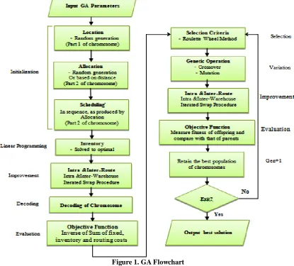
Figure 1. GA Flowchart
4.1. Chromosome representation and encoding
The chromosome representation and encoding of a solution is the first task when utilizing a genetic algorithm. Each chromosome must contain information about warehouse location, retailers’ allocation to warehouses, and routing on each time period.Figure 2 shows a sample of the encoding procedureused in this paper.
Journal of Industrial Engineering and Management Studies (JIEMS), Vol.5, No.1 Page 113 As the figure 2 shown, a chromosome constitutes of 2 warehouses (A and B) and 6 retailers, operating in 2 time periods are considered. Each chromosome is divided into two parts. The first part illustrates the warehouse location and allocation decisions. This part consists of W · T genes. Each W.T genes correspond to a respective time period. The location of the gene is an index corresponding to a candidate warehouse.
The value of that gene is the number of retailers assigned to the warehouse in that particular time period. Warehouse A is open and is serving 4 retailers in time period 1. Also, two retailers are assigned to warehouse B in the same time period. A value of zero means that no retailer is assigned to this warehouse at this time period. In the second time period, warehouse A serves all 6 retailers and no retailers are assigned to warehouse B. However, warehouse B is not closed. Only if all gene values which correspond to the same warehouse across all time periods are zero, is the warehouse assumed closed and no cost of opening and operating of that warehouse is considered.
The second part of the chromosome contains I · T genes. The value of the gene represents the retailer number. The location, however, is related to the assignment to the warehouses as well as to the routing priority. The preference of vehicles for delivering perishable products in the first time periods from warehouse A would be A-3-2-4-6-A. However, vehicle capacity should be considered.
Moreover if the capacity of the vehicle is filled only by the shipment of the requested product of retailers 3 and 2 then totally two or three vehicle would be needed with routing address: A-2-3-A and A-4-6-A or A-A-2-3-A, A-4-A and A-6-A.
In the second time period, all retailers are served by warehouse A. As the previous time period, the number of vehicles is decided by the amount delivering products and by the vehicle capacity.
4.2. Initial population construction
As Fogue et al. (2016) point out the population in genetic algorithms usually contains a fixed number of individuals as well as population includes the candidate individuals corresponding with solutions during a generation. As the initial solutions, a population with the desired number of individuals is randomly generated to start the exploration of near optimum solution. The size of the population affects the speed of the algorithm, since small populations allow higher speeds but make premature convergence of the solutions.
The initial population is generated in two stages. In the first part, chromosome is generated by randomly a number between 0 and I to the first warehouse, and then iteratively generating a random number between 0 and the remaining of the I and assigned to the next warehouse. This pattern continues for the remaining time periods. For the second part, two methods were presented based on random assignments and distance dependent assignments. However the first method is ignored because of the probability of the duplication of the retailer numbers. The second method is based on the distance between warehouses and retailers that proposed by Hiassat and Diabat (2011). In this procedure, each retailer is assigned to the nearest available warehouse. Meanwhile a counter representing the needed assignments for this warehouse is decreased by one. Once the counter reaches zero, the warehouse is removed from the available warehouse list. In generating the initial population, all individuals generated were designed to be feasible. Hence, a mechanism to repair infeasible chromosomes was not needed and, thus, was not implemented.
4.3. Optimal inventory
M.B. Fakhrzad, Z. Alidoosti
with solving an inventory model to optimality. The values of amounts shipped and total inventory cost is taken as inputs to the genetic algorithm. The solution of this inventory model determines the quantities, to be shipped to retailers in each time period.
Inventory Cost = ∑ ∑ hitIit 𝑖∈𝐼
+ ∑ ∑ 𝑝𝑡. 𝑆𝑝𝑖 𝑖∈𝐼
. 𝐼𝑖(𝑡) 𝑡∈𝑇
𝑡∈𝑇
S.t
𝑆𝑝𝑖(𝑡) = 𝑆𝑝𝑖. 𝐼𝑖(𝑡) ∀𝑖 ∈ 𝐼, 𝑡 ∈ 𝑇 (2)
𝐼𝑖𝑡−1+ 𝑎𝑖𝑟𝑡 = 𝑑𝑖𝑡+ 𝐼𝑖𝑡− 𝑆𝑝𝑖(𝑡) ∀𝑖 ∈ 𝐼, 𝑡 ∈ 𝑇 (3)
𝐼𝑖𝑡 ≤ 𝐶𝑖 ∀𝑖 ∈ 𝐼, 𝑡 ∈ 𝑇 (4)
ait, Iit≥ 0 ∀i ∈ I, t ∈ T (5)
4.4. Improvement
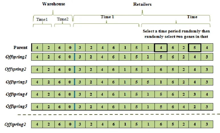
To evaluate theprocedure in the generations of Genetic Algorithm, operators are employed to create a better solution and replace them with those existed. Generally, genetic operators are categorized as selection, crossover and mutation. The initial population and offspring generated by the genetic operations. In addition to these general operators, other methods in each generation could be used that improve chromosomes. Iterated Swap Procedure (ISP) is one of them which was originally developed by Ho. The ISP was employed in developed GA by Hiassat et al. (2011) that is shown in Fig. 3 below.
The ISP procedure operates on the retailers’ part of the chromosome as follows .Step 1: start from the first time period, and select two genes in the retailers’ side. Step 2: exchange the positions of these two genes to form one offspring. Step 3: swap these two genes with their neighbours to form four additional off spring. Step 4: randomly select two genes from the next time period and go back to Step 2.Step 5: evaluate all generated offspring and compare to parent. After the above mentioned procedure the best chromosome is taken, and the rest are rejected. The ISP may exchange genes between retailers assigned to the same warehouse or between different warehouses (intra- or inter-warehouse improvement). Also, the ISP may exchange between retailers within the same route or in two different routes (intra - or inter-route improvement). This interchange, and deciding which of these changes should occur, is governed by the choice of the two genes at the start of the operation.
Journal of Industrial Engineering and Management Studies (JIEMS), Vol.5, No.1 Page 115 4.5. Chromosome decoding
In this section, the variable 𝑋ℎis defined representing a chromosome related to a given individual of the population of period t contained 𝑖 + 𝑤 genes in the decoding process. The value of decision variable 𝑋ℎ is obtained from permutation numbers of the chromosome encoded in the last row as follows.
All cost components involved in the model. This contains the cost of opening and operating a warehouse, known as the fixed cost (FC), the cost of shipping products in terms of cost of routes followed, or routing cost (RC), and the cost of holding products and spoilage products in inventory (HC), known as inventory cost. The cost of warehouse routing is the sum of the cost of all routes for a given warehouse. The sum of such costs over all warehouses constitutes the total routing cost of the chromosome. Let RCh(w)be the total delivery cost needed for warehouse w in chromosome h. If mc is the number of customers in route r and mr is the number of routes in warehouse w, then
𝑅𝐶ℎ(𝑤) = ∑ {𝑐[𝑣(𝑚𝑐), 𝑣(0)] + ∑ 𝑐[𝑣(𝑖 − 1), 𝑣(𝑖)]
𝑚𝑐
𝑖=1
}
𝑚𝑟
𝑟=1
Where v(i)is the location of retailer i, v(0)is the location of the warehouse w,(w = 1, 2, . . ., W), and
𝑐(𝑎, 𝑏) = 𝑝(√(𝑋𝑎− 𝑋𝑏)2+ (𝑌𝑎− 𝑌𝑏)2
is the cost of traveling from point a to point b, where p is a cost factor per unit distance. Therefore, the total routing cost for chromosome h is
𝑅𝐶ℎ = ∑ 𝑅𝐶ℎ(𝑤)
𝑤∈𝑊
And the total cost of all components is
𝑋ℎ = 𝐹𝐶ℎ+ 𝐻𝐶ℎ+ 𝑅𝐶ℎ 4.6. Fitness function
In GAs, the fitness function estimates how close a candidate is to be a solution. Generally, the fitness function should be consistent with better performance.
In our study the fitness function regarding the goal of our problem is inversely related to the summation of all cost components involved in the model for each chromosome. These include the cost of opening and operating a warehouse, k nown as the fixed cost (FC), the cost of shipping products in terms of cost of routes followed, or routing cost (RC), and the cost of holding products and spoiled products in inventory (HC), known as inventory cost. As following proposed formulation the lower costs mean higher fitness function:
𝐹𝑖𝑡𝑡𝑛𝑒𝑠𝑠 𝐹𝑢𝑛𝑐𝑡𝑖𝑜𝑛 = 1/𝑋ℎ 4.7. Selection
M.B. Fakhrzad, Z. Alidoosti
Hence, lower costs mean higher probability to be selected. The procedure of selection commences with the calculation of the total fitness F of a population of size pop size as follows:
𝑭 = ∑ 𝑋ℎ 𝑝𝑜𝑝𝑠𝑖𝑧𝑒
ℎ=1
The selection probability 𝒑𝒉 for each chromosome h is:
𝒑𝒉 =
𝐹 − 𝑋ℎ
𝐹 × (𝑝𝑜𝑝𝑠𝑖𝑧𝑒 − 1)
Then, a random number r is generated in the range (0,1]. If 𝑟 ≤ 𝒒𝒉, then chromosome h is selected.
4.8. Maintaining feasibility
To impose the necessity of satisfaction of the constraints on a problem by evolutionary algorithms, several approaches can be employed. A first approach consists in calculating the fitness function only in the feasible region of function (F). Also the individuals in the infeasible region are neglected. While plenty of studies shown that many feasible global optima are on the boundary of F. Having solution instances on both sides of this boundary can help much to discover these optima. This is more useful when problems have disconnected feasible regions or the optimal solution is at the boundary of the feasible region. However, the final solution must be feasible. As such, various techniques for controlling infeasible chromosomes must be employed. However, in the first approach algorithms maintain only feasible populations all the time. This is accomplished by careful initial population construction, as well as choosing the right main operators.
In this study as previous one, only feasible chromosomes are generated and kept throughout the generations. Due to adopting this approach genetic operations were carefully designed to maintain feasibility of chromosomes.
4.9. Genetic operations
According to some of the studies about genetic operations such as McCal (2005) and Fakhrzad and Moobed (2010), Genetic operators are employed to create a better solution and replace them with those existed in the initial population in order to obtain a near optimum solution. Generally, genetic operators are categorized as selection, crossover and mutation. The search progress is accomplished by crossover and mutation. Both operations constitute the exploitation and exploration part of the search. Because of the type of chromosome structure (warehouse-retailer assignment) in this study repetition of a given time period of a value is not allowed in the second part. As such, genetic operations were carefully designed to create feasible solutions.
4.9.1. Crossover
Journal of Industrial Engineering and Management Studies (JIEMS), Vol.5, No.1 Page 117 This method keeps the offspring feasible. Figure 4 below illustrates an instance of an illegal and legal crossover.
Figure 4. Crossover Operation: (a) Illegal cross over (b) Legal cross over
4.9.2. Mutation
The other genetic operator is a mutation. The mutation operator is traditionally defined as the change probability for a single gene and introduces diversity in the population. The key role of this operator in GA is to avoid local optimization by randomly changing individual genes and expanding the search space.
Also it is employed to explore new solutions in the solution space. Many kinds of mutation operations exist. One of them that used here was Swap mutation, as presented below: 4.9.2.1. Swap mutation
In this process two genes are randomly selected in a time period and they are swapped (by value) in all time periods. For example, if retailers 3 and 5 are selected, then their positions are swapped in all time periods.
5. Results analysis
In this section, a number of randomly generated instances were tested in order to show the performance of the proposed algorithm with considering spoiled product and without spoiled product. To improve the effect of product spoilage as well as approaching the inventory model to the real model, the variable of sale price per each period time was defined. In order to improve the efficiency of product spoilage and approaching inventory model to the real model variable sale price per each period time, was be defined. Particularly, the data was generated as follows: Number of retailers: 4 with 2 warehouses, 6 with 2 warehouses, 8 with 3 warehouses. Location of retailers and warehouses expressed as (𝑿𝒗, 𝒀𝒗) coordinates for node v: random integer in the interval [0,500] Demand of each retailer per time period: random integer in the interval [10,100] Inventory holding cost per time period: random integer in the interval [4.5, 5] Capacity of fleet of vehicles: 110% of total demand of retailers Number of vehicles:
𝑁𝑢𝑚𝑏𝑒𝑟 𝑜𝑓 𝑉𝑒ℎ𝑖𝑐𝑙𝑒 =1.1
𝑐 {∑ ∑ 𝑑𝑖𝑡
𝑡∈𝑇 𝑖∈𝐼
Initial inventory Ii0: random integer in the interval [0, di1+ di2] Number of time periods: 5
Vehicle capacity: 1.5 dmax
Rate of Spoilage of products: %10
Price of products at the beginning of time periods (𝑝𝑡1): 10
Price of products at the end of time periods ( 𝑝𝑡2): 8
As above mentioned, developed model here is NP-hard, therefore GAs as one of the meta-heuristic algorithms could be proposed to solve it. To test its effectiveness, the GA developed here is evaluated with instances of different sizes. Table 1 summarizes the GA parameter set for the genetic algorithm used for testing. The benefit of using the GA is depicted in Figure 5.
Table 1. GA parameters for testing of different sizes
As Figure 5 shown, the graph consists of two lines. The first line is related to the time of running the genetic algorithm on different sized instances. Also the other line associated to the time of running the CPLEX solver in GAMS. In term of difference between two graphs, the running time of instances depicts considerable different between GAMS and GA in the medium- and large-sized instances. Consequently a major advantage of GAs would be the ability to solve medium- and large-sized instances in reasonable time.
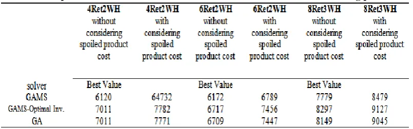
Journal of Industrial Engineering and Management Studies (JIEMS), Vol.5, No.1 Page 119 However, the genetic algorithm is not very efficient in finding the solution for small instances. A summary result of testing models with considering spoiled product and without considering it is shown in Table 2.
The first row represents the result of applying Model 3.3 in GAMS. The second results when restricting the inventory values to be optimal, i.e. setting the variables I it to certain values which correspond to the values found when solving the inventory sub-model 4.3.2. The last value is the average of 30 runs of the GA described earlier.
It is possible to observe that the gap is high for small instances. With medium-sized instances, the gap decreases. This is due to optimizing the inventory in the GA procedure. With larger instances, the effect is suppressed due to other high costs.
Table 2. Comparison of GA solution to other solvers with and without considering products
However, the gap is expected to increase again with large-sized instances as a result of the inevitable existence of many local optima in such large solution spaces. On the other hand, the total cost of the model with considering the cost of the spoiled product and without the cost of the spoiled product is compared. Generally the total cost of the model in the GA is lower than GAMS. As the realistic cost of system was our target, thereby, the total cost of inventory model with deteriorated products is bigger than the others.
6. Conclusion
Generally, the model of location-inventory-routing (LIR) proved substantial cost savings compare to the inventory routing model (IR) which is without the important parameter of the location. Besides, the proposed model in our study showed increase in cost of inventory compare to the previous model that has been recently published. The reason is because of the cost of spoiled products in the model and improving inventory model which would be more realistic than the previous one with only holding inventory costs.Characteristics of this study in comparison with previous studies in this field are presented in Table 2. Proposed future work include using multiple products and accounting for the cost of carbon emissions. The other potential work would be formulating models in all aspects of perishability inventory models that could be categorized in the normal state and critical state such as disaster reliefs with comparing each other. Additionally using the other meta -heuristic search and hybridization with a genetic algorithm such as Taguchi design method or using it lonely such as modified Particle Swarm could be the other future solution methods.
References
Ahmadi-Javid, A., and A.H. Seddighi, (2012). “A location-routing-inventory model for designing multisource distribution networks”, Engineering Optimization, Vol. 44, No. 6, pp. 637-656.
M.B. Fakhrzad, Z. Alidoosti
Brodheim, E., (1975). “On the evaluation of a class of inventory policies for perishable products such as blood”, Management Science, Vol. 21, No. 11, pp. 1320–1325.
Duong, L., (2015). “Multi-criteria inventory management system for perishable & substitutable products”, Procedia Manufacturing, Vol. 2, pp. 66-76.
Forouzanfar, F., and R. Tavakkoli-Moghaddam, (2012). “Using a genetic algorithm to optimize the total cost for a location-routing-inventory problem in a supply chain with risk pooling”, Journal of Applied Operational Research, Vol. 4, No. 1, pp. 2-13.
Fakhrzad, M.B., and A. Sadri Esfahani, (2014). “Modeling the Time Windows Vehicle Routing Problem in Cross-docking Strategy Using Two Meta-heuristic Algorithms”, International Journal of Engineering, Vol. 27, No. 7, pp. 1113-1126.
Fakhrzad, M.B., M.E. Ramazankhani, A. Mostafaeipour, and H. Hosseininasab, (2016). “Feasibility of geothermal power assisted hydrogen production in Iran’, International Journal of Hydrogen Energy, Vol. 41, No. 41, pp. 18351-18369.
Hiassat, (2017). “A genetic algorithm approach for a location-inventory-routing problem with perishable products”, Journal of Manufacturing Systems, Vol. 42, pp. 93–103.
Fakhrzada, M.B., and M. Moobed, (2010). “A GA Model Development for Decision Making Under Reverse Logistics”, International Journal of Industrial Engineering, Vol. 21, No. 4, pp. 211-220. Liu, B., (2015). “A Pseudo-Parallel Genetic Algorithm Integrating Simulated Annealing for Stochastic Location-Inventory-Routing Problem with Consideration of Returns in E-Commerce”, Discrete Dynamics in Nature and Society, pp. 1-15.
Fogue, M., (2016). “Non-emergency patient transport services planning through genetic algorithms”, Expert Systems with Applications, Vol. 61, No. 1, pp. 262-271.
Liu, S., and S. Lee, (2003). “A two-phase heuristic method for the multi-depot location routing problem taking inventory control decisions into consideration”, Int. J. Adv. Manuf. Technol., Vol. 22, pp. 941–950.
Hiassat A, and Diabat A., (2011). “A location-inventory-routing problem with perishable products”, Proceedings of the 41st International Conference on Computers and Industrial Engineering.
Javid, A.A., and N. Azad, (2010). “Incorporating location, routing and inventory decisions in supply chain network design”,Transportation Research Part E: Logistics and Transportation Review, Vol. 46, No. 5, pp. 582–597.
Liu, S., and C. Lin, (2005). “A heuristic method for the combined location routing and inventory problem”, Int. J. Adv. Manuf. Technol, Vol. 26, pp. 372–381.
Le, T., Diabat, (2013). “A column generation-based heuristic algorithm for an inventory routing problem with perishable goods”, Optimization Letters, Vol. 7, No. 7, pp. 1481–1502.
McCal J., (2005). “Genetic algorithms for modelling and optimization”, Journal of Computational and Applied Mathematics, Vol. 184, pp. 205–222.
Mirzaei, S., and A. Seifi (2015). “Considering Lost Sale in Inventory Routing Problems for Perishable Goods”, Computers & Industrial Engineering, Vol. 87, pp. 213-227.
Rayata, F., (2017). “Bi-objective reliable location-inventory-routing problem with partial backordering under disruption risks: a modified AMOSA approach”, Applied Soft Computing; Vol. 59, pp. 622-643.
Journal of Industrial Engineering and Management Studies (JIEMS), Vol.5, No.1 Page 121
Schuster Puga, and M., J. Tancrez, (2017). “A heuristic algorithm for solving large location-inventory problems with demand uncertainty”,European Journal of Operational Research, Vol. 259, pp. 413-423.
Shaabani, H., and I. N. Kamalabadi, (2016). “An efficient population based simulated annealing algorithm for the multi-product multi-retailer perishable inventory routing problem”, Computers & Industrial Engineering, Vol. 99, pp. 189-201.
Shen, Z.J.M., and L. Qi, (2007). “Incorporating inventory and routing costs in strategic location models”, European Journal of Operational Research, Vol. 179, pp. 372–389.
Song, B. D., and Y. D. Ko, (2016). “A vehicle routing problem of both refrigerated- and general-type vehicles for perishable food products delivery”, Journal of Food Engineering, Vol. 169, pp. 61-71.
Tarantilis, C.D., and C.T., Kiranoudis, (2002). “Distribution of fresh meat”, Journal of Food Engineering, Vol. 51, No. 1, pp. 85-91.
Zanoni, S., and L., Zavanella, (2007). “Single-vendor single-buyer with integrated transport inventory system: Models and heuristics in the case of perishable goods”, Computers & Industrial Engineering, Vol. 52, No. 1, pp. 107–123.