https://doi.org/10.5194/wes-3-75-2018
© Author(s) 2018. This work is distributed under the Creative Commons Attribution 4.0 License.
A control-oriented dynamic wind farm model: WFSim
Sjoerd Boersma1, Bart Doekemeijer1, Mehdi Vali2, Johan Meyers3, and Jan-Willem van Wingerden1 1Delft University of Technology, Delft Center for Systems and Control,
Mekelweg 2, 2628 CC, Delft, the Netherlands
2Wind Energy System Research Group, ForWind, Küpkersweg 70, 26129 Oldenburg, Germany 3KU Leuven, Department of Mechanical Engineering, Celestijnenlaan 300A, B3001 Leuven, Belgium
Correspondence:Sjoerd Boersma ([email protected])
Received: 3 October 2017 – Discussion started: 17 October 2017 Revised: 20 January 2018 – Accepted: 6 February 2018 – Published: 6 March 2018
Abstract. Wind turbines are often sited together in wind farms as it is economically advantageous. Control-ling the flow within wind farms to reduce the fatigue loads, maximize energy production and provide ancillary services is a challenging control problem due to the underlying time-varying non-linear wake dynamics. In this paper, we present a control-oriented dynamical wind farm model called the WindFarmSimulator (WFSim) that can be used in closed-loop wind farm control algorithms. The three-dimensional Navier–Stokes equations were the starting point for deriving the control-oriented dynamic wind farm model. Then, in order to reduce computa-tional complexity, terms involving the vertical dimension were either neglected or estimated in order to partially compensate for neglecting the vertical dimension. Sparsity of and structure in the system matrices make this model relatively computationally inexpensive. We showed that by taking the vertical dimension partially into account, the estimation of flow data generated with a high-fidelity wind farm model is improved relative to when the vertical dimension is completely neglected in WFSim. Moreover, we showed that, for the study cases con-sidered in this work, WFSim is potentially fast enough to be used in an online closed-loop control framework including model parameter updates. Finally we showed that the proposed wind farm model is able to estimate flow and power signals generated by two different 3-D high-fidelity wind farm models.
1 Introduction
Optimizing the control of wind turbines in a farm is chal-lenging due to the aerodynamic interactions among tur-bines. These interactions come from the fact that down-wind turbines are often operating in the wakes of updown-wind ones (Barthelmie et al., 2009). Two important wake charac-teristics are (1) a flow velocity deficit and (2) an increase in turbulence intensity. The former reduces power production of the farm while the latter leads to a higher dynamic load-ing on downstream turbines but also induces wake recovery. Individual turbine control variables can influence the wake’s flow velocity, turbulence intensity and also location. Hence, by changing the control variables of individual turbines, power production of and loading on these controlled tur-bines and the downwind turtur-bines can be manipulated. Wind farm control aims to find control variables under changing
the model quality. Modelling is therefore a crucial step to-wards successful implementation of model-based wind farm control.
Overviews on wind farm models can be found in Cre-spo et al. (1999), Vermeer et al. (2003), Sanderse (2009), Sanderse et al. (2011), Annoni et al. (2014), Göçmen at al. (2016) and Boersma et al. (2017). The spectrum of these models ranges from low fidelity to high fidelity. The latter tries to capture relatively precise wind farm flow and tur-bine dynamics, while the former tries to capture only the dominant characteristics (dynamic or static) in a wind farm. Examples of high-fidelity wind farm models are Simulator fOr Wind Farm Applications (SOWFA) (Churchfield et al., 2012), UTD Wind Farm (UTDWF) (Martinez-Tossas et al., 2014), SP-Wind (Meyers and Meneveau, 2010) and PAral-lelized LES Model (PALM) (Maronga et al., 2015). These three dimensional (3-D) high-fidelity wind farm models can easily have 106 or more states. The resulting computation time can be of the order of days or weeks using distributed computation for simulation times less than the computation time. In other words, the computation time needed for large-eddy simulations (LESs) is in general more than the total time that is simulated. Clearly, these types of models are not applicable for online model-based control. Rather, these models serve as analysis or validation tools.
One way to reduce the high complexity of wake mod-elling is by using two-dimensional (2-D) heuristic models that only capture specific wake and turbine characteristics in a wind farm in the horizontal plane at hub height. These types of models are found on the low-fidelity side of the spectrum. Most of these wake models exclusively estimate a steady state situation for given atmospheric conditions. Ex-amples of static models are the Frandsen model (Frandsen et al., 2006) and the Jensen–Park model (Jensen, 1983; Katic et al., 1986). One extension of the Jensen model resulted in the parametric model called FLOw Redirection and In-duction in Steady-state (FLORIS) (Gebraad et al., 2014b). Two examples of low-fidelity dynamic models are SimWind-Farm (Grunnet et al., 2010) and the model used in Shapiro et al. (2017a), in which relatively simple approximations of the flow deficit are computed using heuristic expressions.
Medium-fidelity models can be found in the middle of the spectrum as they trade off the accuracy of high-fidelity models with the computational complexity of low-fidelity models. These are in general based on simplified versions of the Navier–Stokes equations. For example, in the 2-D dy-namic wake meandering (DWM) model (Larsen et al., 2007), assumptions are made regarding the thin shear layer such that the Navier–Stokes equations can be approximated us-ing less computational effort. The authors in Trabucchi et al. (2016) present a model, which is also based on the thin shear layer approximation, but according to the authors it is ap-plicable for non-axisymmetric wind turbine wakes. Wake-Farm (also referred to as Wake-FarmFlow) simulates the wind turbine wakes by solving the steady parabolized Navier–
Stokes equations in three dimensions (Crespo et al., 1988; Özdemir et al., 2013). Other wind farm models based on the 3-D Reynolds-averaged Navier–Stokes (RANS) equa-tions are Avila et al. (2013) and van der Laan et al. (2015). In Annoni and Seiler (2015), time averaging is applied to the Navier–Stokes equations, resulting in the 2-D RANS equa-tions. The number of states is then reduced by employing a state reduction technique.
Also considered as medium-fidelity models are the ones presented in Boersma et al. (2016b) and Soleimanzadeh et al. (2014). These wind farm models are based on the dis-cretized 2-D Navier–Stokes equations. However, these mod-els do not contain a turbulence model that allows for wake recovery. In addition, these 2-D models do not take any ne-glected 3-D effects into account and no yaw actuation of the individual turbines is included.
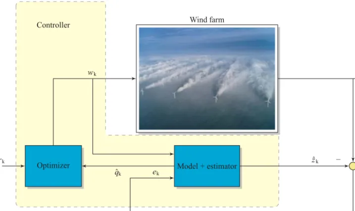
In this paper, a model will be presented that can be consid-ered as a building block for the closed-loop control frame-work as illustrated in Fig. 1.
In current practice, signals such as power can be measured from a wind farm, but current research is also focussing on estimating wake characteristics using a lidar device (Raach et al., 2017). These and other wind farm measurements are called SCADA data and can be used by an estimator that is able to adapt the model parameters to current atmospheric conditions and/or estimate the full state space, e.g. all the flow velocities at hub height in the farm. The work presented in Doekemeijer et al. (2016) illustrates the latter and employs the dynamic wind farm model presented in this paper. Sub-sequently, the estimation can then be used to compute op-timal control variables using a model predictive controller. The work presented in Vali et al. (2016) illustrates the appli-cation of such a model predictive wind farm controller using the dynamic model presented in this work.
The online closed-loop control paradigm as depicted in Fig. 1 demands a control-oriented dynamic wind farm model that will be presented in this paper. Characteristics of such control-oriented models are
1. low computational cost such that online model update, state estimation and control signal evaluation is possi-ble;
2. their dynamical nature such that they can deal with varying atmospheric conditions within relatively small timescales.
fea-Wind farm
wk zk
Model + estimator zˆk −
+
ek
Optimizer
ˆ qk rk
Controller
Figure 1.General dynamical closed-loop control framework with measurementszkand its estimationzˆkand state estimationqˆk. The signals rkandwkare reference and control signals, respectively. In this paper we present a dynamic model that is compatible with this framework.
ture is the exploitation of the sparse system matrices, lead-ing to computational efficiency. WFSim will be compared to high-fidelity flow data and used in a practical control appli-cation.
The remainder of this paper is organized as follows. In Sect. 2, the mathematical background of the medium-fidelity wind farm model will be explained including a discussion on the rotor and turbulence model. This section ends with an analysis regarding the wind farm model’s computation time. In Sect. 3, WFSim will be validated in two cases us-ing flow velocities in the longitudinal and lateral directions at hub height and turbine power signals computed with two different LES-based wind farm models. The first case consid-ered is a two-turbine wind farm with turbines modelled using the ADM. The second case is a nine-turbine wind farm with turbines modelled employing Fatigue, Aerodynamics, Struc-tures and Turbulence (FAST) (Jonkman and Buhl, 2005). This paper is concluded in Sect. 4.
2 Formulation of a dynamic control-oriented wind farm model
In the current section, a simplified wind farm model is for-mulated that is sufficiently fast for online control but retains some of the elemental features of three-dimensional turbu-lent flows. In order for the model to be fast, we envisage a 2-D-like model, but adapted to account for three-dimensional flow relaxation. We will dub the resulting model WFSim (WindFarmSimulator).
As a starting point we use the standard incompressible three-dimensional filtered Navier–Stokes equations, as used in LES, i.e.
∂ev
∂t +(ev· ∇)ev+ ∇ ·τM+ 1
ρ∇pe−f=0, momentum equation,
∇ ·
ev=0,
continuity equation.
(1)
The velocity fieldev=(ev1,ev2,ev3)
T and pressure field e p rep-resent filtered variables; ∇ =(∂/∂x, ∂/∂y, ∂/∂z)T; the air density ρ, which is assumed to be constant; and τM
rep-resents the subgrid-scale model, which will be defined in Sect. 2.1. As is common in LESs of high-Reynolds-number atmospheric simulations with grid resolutions in the metre range, direct effects of viscous stresses on the filtered fields are negligible, so that these terms are left out. Finally, the termf represents the effect of turbines on the flow, as fur-ther detailed in Sect. 2.2.
Although LES filters are usually implicitly tied to the LES grid and filter length scale in the subgrid-scale model, we presume here thatevcorresponds to a top-hat filtered velocity field, with filter widthD, whereD is the turbine diameter. Thus,
ev(x, y, z)= 1 D3
z+D/2
Z
z−D/2 y+D/2
Z
y−D/2 x+D/2
Z
x−D/2
v(x0, y0, z0) dx0dy0dz0. (2)
(xn, yn)T (withn=1· · ·ℵ andℵ the number of turbines in the farm) sinceev(xn, yn, zh) is a reasonable representation of
the turbine disk-averaged velocity.
Therefore, we focus on formulating a 2-D-like set of equa-tions forev(x, y, zh). To this end, we define
u=
ev1(x, y, zh) ev2(x, y, zh) T
, (3)
= u vT, (4)
and w=
ev3(x, y, zh) and p=p(x, y, ze h)/ρ. Moreover, we assume thatw≈0, so that the LES equations given in Eq. (1) can be reformulated in terms ofuas
∂u
∂t +(u· ∇H)u+ ∇H·τH+ ∇Hp−f
= −∂(uw+τM,13)
∂z e1−
∂(vw+τM,23)
∂z e2, (5)
∇H·u= −∂w
∂z, (6)
with ∇H=(∂/∂x, ∂/∂y)T,τH a 2-D tensor containing the
horizontal components of the subgrid stressesτM, ande1and
e2the unit vectors in thexandydirections, respectively.
Finally, we further simplify the equations above using two additional assumptions. First of all, we presume ∂w/∂z≈
∂v/∂y. When centred at the turbine axis, this is one of the conditions required for axial symmetry, though axial sym-metry also requires further conditions on∂v/∂zand∂w/∂y, which are not imposed. In general,∂w/∂z≈∂v/∂yimplies equal divergence–convergence of streamlines iny andz di-rections. Although this is a very simple condition, we pre-sume it to be good enough to resolve the lack of relaxation of purely 2-D models. If necessary, a more general form (w≈0 and∂w/∂z≈c·∂v/∂y), withca tuning parameter (e.g. ob-tained through state estimation) could be considered, but re-sults in the current work indicate that this may not be nec-essary. Secondly, we simply neglect the right-hand side of Eq. (5). Though this is a rather crude assumption, the ratio-nale is that the modelling term τH will suffice in the
con-text of a control model, where model coefficients can be up-dated online based on feedback (see also the discussion in Sect. 2.1). Hence our final 2-D-like model corresponds to
∂u
∂t +(u· ∇H)u+ ∇H·τH+ ∇Hp−f =0, (7)
∇H·u= −∂v
∂y. (8)
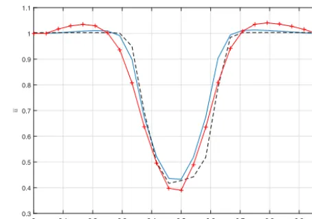
We emphasize here that the model above is not a classical 2-D model due to the difference in formulation of the con-tinuity equation. In contrast to a standard 2-D model, this allows for flow relaxation in the third direction when, for example, encountering slow down by a wind turbine. This can be seen in Fig. 2, in which simulation results obtained with the model above, a standard 2-D dynamic wind farm model and LES are shown. The simulation case itself will
0 0.1 0.2 0.3 0.4 0.5 0.6 0.7 0.8 0.9 1
y 0.3
0.4 0.5 0.6 0.7 0.8 0.9 1 1.1
u
Figure 2.Results of two-turbine simulations. Normalized time-averaged wake deficit at hub height 5Ddownwind from the down-wind turbine using standard 2-D Navier–Stokes equations (red crossed), our model with the adapted continuity equation (blue), and LES data (black dashed).
be discussed in more detail in Sect. 3.2.1. Here we depict the normalized flow deficit in the wake at 5Ddownstream of the turbine along the cross-stream axis. The figure illus-trates that the standard 2-D Navier–Stokes equations lead to a significant speed up at the wake edges. This is a result from conservation of mass in two dimensions and the flow decel-eration in front of the turbine, pushing part of the air around the turbine. In the WFSim model, this speed up is smaller, as mass can also flow around the turbine in the third dimen-sion. In Fig. 2 it can be seen that LES data are better esti-mated when imposing flow relaxation in the third dimension. Finally, note that partially modelling the missing vertical di-mension as proposed above is novel with respect to the work presented in Boersma et al. (2016a).
This section is further organized as follows. First, in Sect. 2.1, the subgrid-scale model will be introduced. Then, in Sect. 2.2, the turbine model will be explained. The dis-cretization of the equations is presented in Sect. 2.4, and boundary and initial conditions are discussed in Sect. 2.5.
2.1 Turbulence model
1 1
2 2
3 3
Figure 3.Schematic illustration of the mixing length.
We formulate the stress tensorτHusing an eddy-viscosity
assumption, i.e.
τH= −νtS, (9)
with S=1
2(∇Hu+(∇Hu)T) the 2-D rate-of-strain tensor,
andνt the eddy viscosity. The latter is further modelled as in Prandtl (1925):
νt=lu(x, y)2
∂u ∂y
, (10)
wherelu(x, y) is the mixing length. It could be interesting to define the mixing length for each position in the wind farm separately, but this will lead to too many tuning variables. Moreover, in Iungo et al. (2015), the authors illustrate that in a turbine’s near wake the mixing length is roughly invariant for different downstream locations, but in the far wake, the mixing length increases linearly with downstream distance. We use this to formulate a simple heuristic parametrization for the mixing length model so that the number of decision variables will be reduced drastically. From now on we as-sume that the wind is coming from the east, but can have a direction defined byϕ. Then, the wind farm will be divided in segments as illustrated in Fig. 3.
Each segments has its own (x0n, y0n) coordinate system lo-cated in the global (x, y) coordinate system. Now we propose the following mixing length parametrization:
lu(x, y)=
G(x0
n, yn0)∗lnu(xn0, yn0), ifx∈X andy∈Y.
0, otherwise, (11)
with G(x, y) a (smoothing) pillbox filter with radius 3, ∗
the 2-D spatial convolution operator, X = {x : xn0 ≤x≤
xn0+cos(ϕ)d},Y= {y : yn0−D
2+sin(ϕ)x 0
n≤y≤y 0 n+D2+
sin(ϕ)xn0} and ϕ defined as the mean wind direction (see Fig. 3), which we bound by|ϕ| ≤45◦in this work. In addi-tion we constraintdby cos(ϕ)d≤ |xq−xn|, withxna turbine x coordinate andxqits downwind turbinesxcoordinate. We can seelun(xn0, yn0) as the local mixing length that belongs to
turbinenand denote it as
lun(xn0, yn0)=
(
(xn0−d0)ls, ifxn0 ∈Xn0andyn0 ∈Yn0.
0, otherwise. (12)
with X0 n= {x
0 n : d
0≤x0
n≤d} and Y 0 n= {y
0 n : |y
0 n| ≤D} and tuning parameterls that defines the slope of the (lin-early increasing) local mixing length parameter. In fact, this parameter could be related to turbulence intensity, i.e., the amount of wake recovery. In this work we will not investigate this relation further. With the formulation above, the num-ber of tuning variables that belong to the turbulence model (ls, d, d0) is reduced to 3ℵ. Additionally, we assume thatls, d andd0 are equal for each turbine in the farm, which re-duces the number of tuning variables that belong to the tur-bulence model to three, a quantity that could be dealt with by an online estimator. However, in order to have only three tuning variables, the included turbulence model is defined as a simplified mixing length model found heuristically using and adapting information from Iungo et al. (2015).
2.2 Turbine model
Turbines are modelled using a classical non-rotating actua-tor disk model (ADM). In this method, each wind turbine is represented by a uniformly distributed force acting on the grid points where the rotor disk is located. Figure 4 depicts a schematic top-view representation of a turbine with yaw angleγ.
Using such an approach, the force exerted by the turbines can be expressed as
f=
ℵ X
n=1
fn, with
fn=cf
2 C
0
Tn[Uncos(γn)]
2
cos(γn+ϕ) sin(γn+ϕ)
×H
D
2 − ||s−tn||2
δ
Figure 4.Schematic representation of a turbine with yaw angleγn and flow velocityU=([u(xn, yn)]2+ [v(xn, yn)]2)1/2at the rotor. Figure adapted from Jiménez et al. (2010).
with s=(x, y)T, H[·] the Heaviside function and δ[·] the Dirac delta function, e⊥,n the unit vector perpendicular to the nth rotor disk with position tn. Furthermore, we have CT0
n the disk-based thrust coefficient following Meyers and
Meneveau (2010), which can be expressed in terms of the classical thrust coefficientCTn using the following relation:
CT0
n=CTn/(1−an)
2, witha
nthe axial induction factor of the nth turbine. Interestingly, the coefficientC0T
ncan be directly
related to the turbine set point in terms of blade pitch angle and rotational speed (see, e.g. Appendix A in Goit and Mey-ers, 2015). In the WFSim model,CT0
n and yaw angleγn are
considered as the control variables and can thus be used to regulate the wakes and hence wind farm performance. Fur-thermore, the scalarcf in Eq. (13) can be regarded as a tun-ing variable and will in this work be set equal for all turbines in the farm.
2.3 Power
From the resolved flow velocity components, the power gen-erated by the farm is computed as
P =
ℵ X
n=1
1
2ρA CPn[Uncos(γn)]
3. (14)
It is stated in Goit and Meyers (2015) (Appendix A) that when there is no drag and swirl is added to the wake,CT0
n=
CPn. Since this is an idealized situation, a loss factor will be
introduced such thatCPn=cpC
0
Tn. The scalarcpcan be seen
as a tuning variable and will be set equal for all turbines in the farm. In the power expression above, we have the fac-tor cos(γn)3 with exponent 3. In literature such as Gebraad et al. (2014a) and Medici (2005, p. 37), for example, numeri-cal values for the exponent were given according to LES and wind tunnel data, respectively. However, to date, the exact value for it is still under research and since this is outside the scope of this study, the value of the exponent will be 3.
This concludes the formulation of the WFSim model. In order to resolve for flow velocity components and wind farm
Figure 5.One cell for thexmomentum equation (grey,ui,J), one for theymomentum equation (yellow,vI,j) and one for the conti-nuity equation (pink,pI,J). All three cells have equal dimensions and overlap.
power, the governing equations given in Eqs. (7) and (8) need to be discretized, a topic that will be discussed in the follow-ing section.
2.4 Discretization
The set of equations are spatially discretized over a stag-gered grid following Versteeg and Malalasekera (2007). This is carried out by employing the finite volume method and the hybrid differencing scheme. Temporal discretization is per-formed using the implicit method that is unconditionally sta-ble (Versteeg and Malalasekera, 2007). This comes down to deriving the integrals:
Z
1t Z
1V ∂u
∂t +(u· ∇H)u+ ∇H·τH+ ∇Hp−f
dVdt=0,
Z
1t Z
1V
∇H·u+∂v
∂y
dVdt=0, (15)
with1V the volume of one cell (see Fig. 5) and1tthe sam-ple period. One obtains, for each cell, the following fully dis-cretized Navier–Stokes equations (for detailed derivation we refer to Appendix A):
– x momentum equation for the (i, J)th cell (black in Fig. 5):
ai,Jpxui,J = ai,Jnx a sx i,J a
wx i,J a
ex i,J
× ui,J+1 ui,J−1 ui−1,J ui+1,JT
−δyj,j+1 pI,J−pI−1,J
. . .+ ai,Jnwx ai,Jswx ai,Jnex asexi,J
× vI−1,j+1 vI−1,j vI,j+1 vI,J T
(16)
– y momentum equation for the (I, j)th cell (yellow in Fig. 5):
aI,jpyvI,j =
aI,jny aI,jsy aI,jwy aI,jey
× vI,j+1 vI,j−1 vI−1,j vI+1,j T
−δxi,i+1 pI,J−pI,J−1+fI,jy +. . .
. . .+ ai,Jnwy ai,Jswy aneyi,J ai,Jsey
× ui,J ui,J−1 ui+1,J ui+1,J−1T (17)
– continuity equation for the (I, J)th cell (pink in Fig. 5): 0=δyj,j+1 ui+1,J−ui,J+2δxi,i+1 vI,j+1−vI,j. (18)
The statesu•,•, v•,•, p•,•are defined for the timek+1 while
the coefficientsa••,•and the forcing termsf••,•depend on the state at timek. Detailed definitions of these coefficients are given in Appendix A, Table A1. Note the appearance of the previously explained factor 2 (see Eq. 8) in Eq. (18).
Next, the state vectorsuk, vk, andpk and control variable vectorsνkandγkat time stepkwill be defined:
uk=
u3,2 .. . u3,Ny−1
u4,2 .. . u4,Ny−1
.. . uNx−1,2
.. . uNx−1,Ny−1
, vk=
v2,3 .. . v2,Ny−1
v3,3 .. . v3,Ny−1
.. . vNx−1,3
.. . vNx−1,Ny−1
,
pk=
p2,2 .. . p2,Ny−1
p3,2 .. . p3,Ny−1
.. . pNx−1,3
.. . pNx−1,Ny−2
, νk=
CT0
1
CT0
2
.. . CT0
ℵ
, γk=
γ1 γ2 .. . γℵ , (19)
withNxandNythe number of cells in thexandydirections, respectively, andℵthe number of turbines in the wind farm.
Each component inuk,vk andpk represents a flow velocity and pressure at a point in the field defined by the subscript. For clarity reasons, an example of a staggered grid is depicted in Fig. 6.
2.5 Boundary and initial conditions
All the components that are not contained in the vector,uk, vk andpk, but do appear in the staggered grid need to be de-fined. For the flow velocity components, first-order condi-tions on the west side of the grid are prescribed assuming the wind is coming from the east. These Dirichlet inflow bound-ary conditions are related to the ambient inflow defined asub
andvband can vary over time. Zero stress (also referred to as
Neumann) boundary conditions are prescribed on the other boundaries. Therefore, for the flow velocity components on the boundaries we define
u2,J=ub forJ=1,2, . . ., Ny, ui,Ny =ui,Ny−1 fori=3,4, . . ., Nx,
ui,1=ui,2 fori=3,4, . . ., Nx, uNx,J =uNx−1,J forJ=2,3, . . ., Nx−1,
v1,j=vb forj=2,3, . . ., Ny, vI,Ny =vI,Ny−1 forI=2,3, . . ., Nx,
vI,2=vI,3 forI=2,3, . . ., Nx, vNx,j=vNx−1,j forj=3,4, . . ., Ny−1.
For the initial conditions, we define all longitudinal and latitudinal flow velocity components in the field asub and
vb, respectively, which are the boundary velocity values. The
initial pressure field is set to zero. Note that by defining the boundary conditions as given above, the assumption is that the wind is coming from the east in Fig. 6, which coincides with the definition of the mixing length (see Sect. 2.1). Fi-nally, the equations given in Eqs. (7) and (8) can be trans-formed to the difference algebraic equation1:
Ax(uk, vk) Axy(uk) B1
Ayx(uk) Ay(uk, vk) B2
B1T 2B2T 0
| {z }
E(qk)
uk+1
vk+1
pk+1
| {z } qk+1
=
A11 0 0
0 A22 0
0 0 0
| {z }
A uk vk pk
| {z } qk
+
b1(uk, vk, νk, γk) b2(uk, vk, νk, γk)
b3
| {z }
b(qk,wk)
, (20)
with nq=nu+nv+np and uk∈Rnu, vk∈Rnv, pk∈Rnp containing all flow velocities in the longitudinal and lateral
I= 1 i= 2 I= 2 i= 3 I= 3 i= 4 I= 4 i= 5 I= 5
J= 1
J= 2
J= 3
J= 4
J= 5
j= 2
j= 3
j= 4
j= 5
p2,2
p2,3
p2,4
p3,2
p3,3
p3,4
p4,2
p4,3
p4,4
v1,2 v1,3 v1,4 v1,5
v2,2 v2,3 v2,4 v2,5
v3,2 v3,3 v3,4 v3,5
v4,2 v4,3 v4,4 v4,5
v5,2 v5,3 v5,4 v5,5
u2,1 u2,2 u2,3 u2,4 u2,5
u3,1 u3,2 u3,3 u3,4 u3,5
u4,1 u4,2 u4,3 u4,4 u4,5
u5,1 u5,2 u5,3 u5,4 u5,5
p3,2
u3,2 uu
u u p2,3
v2,3 p
v
p3,3
v3,3
u3,3 p
v
u u
u u
Δx2,3 δx4,5
Δy2,3 δy4,5
Figure 6.Example of a staggered grid with cells each having volume1V. In WFSim, the grid is quadrilateral.
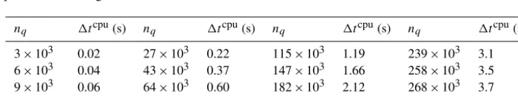
Table 1.Mean computation time per simulation time step1tcpuvs. number of statesnqfor the WFSim representation as given in Eq. (21). Computations are performed on a regular notebook with one core.
nq 1tcpu(s) nq 1tcpu(s) nq 1tcpu(s) nq 1tcpu(s) 3×10³ 0.02 27×103 0.22 115×103 1.19 239×103 3.1 6×10³ 0.04 43×103 0.37 147×103 1.66 258×103 3.5 9×10³ 0.06 64×103 0.60 182×103 2.12 268×103 3.7 14×103 0.10 88×103 0.88 221×103 2.50 276×103 3.8
direction and the pressure vector at timekand control vari-able wk= νkT γkT
T
∈R2ℵ. The non-singular square de-scriptor matrix E(qk) contains the coefficientsa••,•,
appear-ing in Eqs. (16) and (17), that depend on the state at timek. The square constant matrixAsolely depends on grid spac-ing and sample period1t. Note that the state vector contains three states for every cell; hence an increase in grid resolu-tion results in an increase in matrix dimensions. However, the system matrices that occur in Eq. (20) are sparse and efficient numerical solvers are available for these types of problems. This will be demonstrated in Sect. 2.6. The vector b(qk, wk) contains the forcing terms (turbines) and boundary conditions.
By defining Nx, Ny, 1xI,I+1, 1yJ,J+1, and the turbine
positions, a wind farm topology is determined. Next, ambient flow conditionsubandvb, tuning parameterscf, cp, d, d0, ls
and the control variablewkneed to be specified. The system given in Eq. (20) is then fully defined and can be solved.
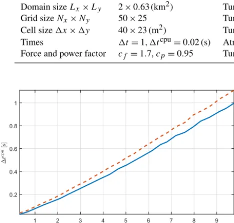
2.6 Computation time
When discretizing partial differential equations, a trade-off has to be made between the computation time and grid reso-lution. Typically, a higher resolution results in more precise computation of the variables but also increasing computa-tion time. In WFSim, computacomputa-tional cost is reduced by ex-ploiting sparsity and by applying the reverse Cuthill–McKee algorithm (George and Liu, 1981).2The latter is applicable due to the fact that the matrix structure is fixed. The
Table 2.Summary of the WFSim simulation set-up.
Domain sizeLx×Ly 2×0.63 (km2) Turbine rotor diameterD 126.4 (m) Grid sizeNx×Ny 50×25 Turbine arrangement 2×1 Cell size1x×1y 40×23 (m2) Turbine spacing 5D
Times 1t=1, 1tcpu=0.02 (s) Atmospheric conditions ub=8,vb=0 (m s−1),ρ=1.2 (kg m−3) Force and power factor cf =1.7,cp=0.95 Turbulence model d=530,d0=122 (m)ls=0.06
1 2 3 4 5 6 7 8 9
× 104
0.2 0.4 0.6 0.8 1
Figure 7.Mean computation time per simulation time step1tcpu vs. number of statesnq. The red dashed line is WFSim as presented in Eq. (20) and blue is WFSim as presented in Eq. (21). Note that the number of cells is approximatelynq/3 withnq the number of states.
ested reader is referred to Doekemeijer et al. (2016) for more information on the Cuthill–McKee algorithm in WFSim.
In this section, the mean computation time needed for one time step1tcpu will be analysed. The presented results are obtained on a regular notebook with an Intel Core i7-4600U 2.7 GHz processor employing one core and MATLAB. Since the objective is to do online control, i.e., it is desired to reduce computational complexity, this section introduces a second WFSim representation. The first representation was given in Eq. (20) while the second is defined as
Ax(uk, vk) 0 B1
0 Ay(uk, vk) B2
B1T 2B2T 0
| {z }
E(qk)
uk+1
vk+1
pk+1
| {z } qk+1
=
A11 0 0
0 A22 0
0 0 0
| {z }
A
uk vk pk
| {z } qk
+
b1(uk, vk, νk, γk) b2(uk, vk, νk, γk)
b3
| {z }
b(qk,wk)
. (21)
The difference can be found in the descriptor matrix. In the representation above, the elementsAxy(uk), Ayx(uk) that oc-cur in Eq. (20) are set to zero. This can be justified by the fact that their contribution is negligible since these matrices contain elements that, for our case studies, are of the order ofO(1) while the elements inAx(uk, vk) andAy(uk, vk) are
of the order ofO(3). Consequently, no significant change in the computed flow field has been observed, but a decrease in1tcpu has (see Fig. 7). Therefore, the remainder of this paper will continue with the WFSim representation given in Eq. (21). Table 1 depicts more numerical values of1tcpufor this WFSim representation.
From Table 1 we can conclude that1tcpu increases be-tween quadratic and linear with respect to the number of states nq for nq<221×103. It depends on the computer properties how much you can increase the number of states until the CPU is out of memory.
3 Simulation results
In this section, WFSim flow and power data will be compared with LES data and it is organized as follows. In Sect. 3.1, quality measures are introduced. In Sect. 3.2.1, WFSim data are compared with PALM data, and in Sect. 3.2.2 WFSim is validated against SOWFA data. In both simulation cases, the thrust coefficientsC0T are varied while the yaw angles are set to zero.
3.1 Quality measures
Suppose we have at timeka measurement of one quantity zk∈RN and its estimation zˆk∈RN. Define the prediction errorek= ˆzk−zk. The quality measure RMSE is, for time stepk, defined as
RMSE(zk,zˆk)= r
1
Ne T
kek. (22)
This measure is used to compare the flow centreline veloc-ityUkc(x) and power signals from LES and WFSim data for different model parameters. The flow centreline is, for one time step, defined as the laterally averaged longitudinal flow velocity throughout the simulation domain across the rotor diameter. Mathematically this can, for LES data at time step kat longitudinal positionxi, be defined as
Ukc(xi)= 1 Ny
Ny
X
s=1
uk(xi, ys), (23)
0 200 400 600 800 1000 1200 1400 1600
t[s] 0
0.5 1 1.5
CT
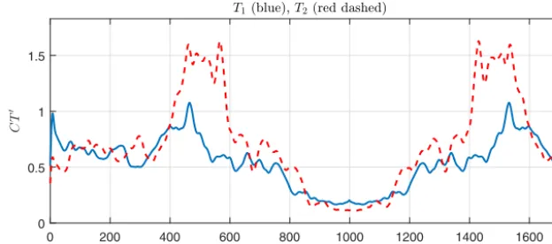
T1(blue),T2(red dashed)
Figure 8.Excitation signals for the two-turbine simulation case. The yaw angles are set to zero.
500 1000 1500 2000 2
4 6 8
U
c[m
s
-1]
t= 300 [s]
500 1000 1500 2000 2
4 6 8
t= 400 [s]
500 1000 1500 2000
x[m]
2
4 6 8
U
c[m
s
-1]
t= 700 [s]
500 1000 1500 2000
x[m]
2 4 6 8
t= 800 [s] WFSim (black) and PALM (blue dashed)
Figure 9.Mean flow centreline at four time instances through the farm. The vertical red dashed lines indicate the positions of the tur-bines.
In this work we compare lateral and longitudinal flow ve-locity components at hub height and power signals calculated with LES with lateral and longitudinal flow velocity compo-nents and power signals calculated with WFSim.3
3.2 Axial induction actuation
Studies such as Shapiro et al. (2017a), Munters and Meyers (2017), Vali et al. (2017) and van Wingerden et al. (2017) illustrate that axial induction actuation can be used in active power control where the objective is to provide grid facil-ities. In order to utilize the WFSim model in active power control, it is important to first validate it when exciting the thrust coefficient.
3The LES flow data are mapped onto the grid of WFSim using bilinear interpolation techniques.
In the following, WFSim is compared with simulation data from PALM (Maronga et al., 2015) and SOWFA (Church-field et al., 2012), both high-fidelity wind farm models that were briefly discussed in Sect. 1. The latter includes the actu-ator line model (ALM) while the former employs the ADM.4
3.2.1 PArallelized LES Model (PALM) and WFSim
PALM predicts the 3-D flow velocity vectors and turbine power signals in a wind farm using LES and is based on the 3-D incompressible Navier–Stokes equations.5 Table 2 gives a summary of the two-turbine wind farm simulated in WFSim. A summary of the PALM simulation set-up can be found in Appendix B. The applied control signals are de-picted in Fig. 8 and are chosen such that different system dynamics are excited. The final values for the tuning param-eters are obtained using a grid search. Figures 9 and 10 show a comparison of the mean flow centreline and the wind farm power, respectively. A flow field evaluated with both the WF-Sim model and PALM can be found in Appendix B.
In Fig. 9, the mean flow centrelines through the farms of WFSim and PALM are relatively similar. The PALM data exhibit more turbulent fluctuations due to the presence of a more sophisticated turbulence model, which allows for bet-ter capturing small-scale dynamics such as turbine-induced turbulence. However, the WFSim model is capable of esti-mating wake recovery similar to the PALM model. The re-covery in the WFSim model is due to the turbulence model as presented in Sect. 2.1. It is in fact the slope of the local mixing length parameters that can determine the amount of wake recovery, or more precisely, the larger this slope, the higher the wake recovery. It is therefore interesting to link this tuning variable to the turbulence intensity in the farm. Furthermore, it can be seen in Fig. 10 that the WFSim model
4PALM also includes the rotating ADM, but in our case study the ADM is employed.
0 200 400 600 800 1000 1200 1400 1600 t[s]
0.5 1 1.5 2 2.5 3
P
[W
]
× 106 Wind farm power: WFSim (black) PALM (blue dashed)
Figure 10.Wind farm power from PALM (blue dashed) and WFSim (black).
0 200 400 600 800 1000
t[s] 0.2
0.4 0.6 0.8 1
CT
T1(blue dashed),T2(black crossed),T3(red)
0 200 400 600 800 1000
t[s] 0.1
0.2 0.3 0.4 0.5 0.6 0.7
0.8 T4(blue dashed),T5(black crossed),T6(red)
0 200 400 600 800 1000
t[s] 0.2
0.4 0.6 0.8 1 1.2 1.4
1.6 T7(blue dashed),T8(black crossed),T9(red)
Figure 11.Excitation signals for the nine-turbine simulation case. The yaw angels are set to zero.
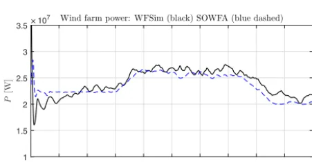
is capable of estimating the wind farm power. Since both the WFSim model and PALM employ the ADM, fast fluctuations in the power signal can be observed. This is due to the lack of rotor inertia in both simulation cases. The simulation case presented in this section illustrates that the WFSim model, in which the third dimension is partially neglected, is able to estimate wind farm flow and power signals computed with a 3-D LES wind farm model. In Sect. 3.2.2, a SOWFA case study will be presented, a LES model that includes turbine dynamics.
3.2.2 Simulator fOr Wind Farm Applications (SOWFA) and WFSim
SOWFA predicts the 3-D flow velocity vectors in a wind farm using LES and is based on the 3-D incompressible Navier–Stokes equations. For turbine modelling it employs the ALM, which is a more sophisticated model than the ADM (Sanderse et al., 2011). In addition, the FAST model from the National Renewable Energy Laboratory (NREL) is implemented (Jonkman and Buhl, 2005). This model cal-culates turbine power production, blade forces on the flow and structural loading on the turbine. In the SOWFA
sim-ulation presented, the NREL 5 MW wind turbine is simu-lated (Jonkman et al., 2009).
The SOWFA data set used in this work for validation is equivalent to the set used in van Wingerden et al. (2017). The thrust coefficientCT0 is not a control variable in SOWFA due to the employment of the ALM and therefore has to be estimated. This will be discussed in the following paragraph.
Turbine operating settings
For estimating the control signalsC0T
n, the turbine’s fore-aft
bending momentMsowfak calculated with FAST is exploited. Using the relationMsowfak =Fsowfak zhwithzhthe hub height,
the (indirect) measured thrust force Fsowfak can be derived. An estimation from SOWFA data of the rotor flow veloc-ityUksowfa is obtained by averaging the flow velocity com-ponents across the rotor. Using the standard ADM yields for each turbine
Fsowfak =1
2AρC
0 T h
Uksowfai2
cos(γk+ϕk) sin(γk+ϕk)
. (24)
Table 3.Summary of the WFSim simulation set-up.
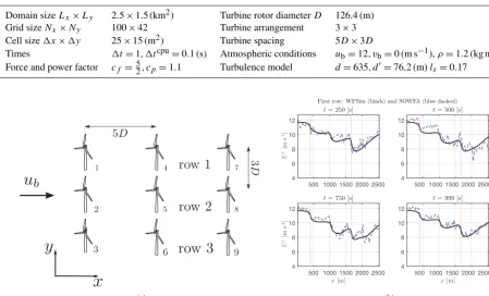
Domain sizeLx×Ly 2.5×1.5 (km2) Turbine rotor diameterD 126.4 (m) Grid sizeNx×Ny 100×42 Turbine arrangement 3×3 Cell size1x×1y 25×15 (m2) Turbine spacing 5D×3D
Times 1t=1, 1tcpu=0.1 (s) Atmospheric conditions ub=12, vb=0 (m s−1),ρ=1.2 (kg m−3) Force and power factor cf =52, cp=1.1 Turbulence model d=635, d
0=
76.2 (m)ls=0.17
(a)
500 1000 1500 2000 2500 4
6 8 10 12
U
c[m
s
-1]
t= 250 [s]
500 1000 1500 2000 2500 4
6 8 10 12
t= 500 [s]
500 1000 1500 2000 2500
x[m]
4 6 8 10 12
U
c[m
s
-1]
t= 750 [s]
500 1000 1500 2000 2500
x[m]
4 6 8 10 12
t= 999 [s] First row: WFSim (black) and SOWFA (blue dashed)
(b)
Figure 12.Topology simulated wind farm(a)and mean flow centreline at four time instances through the first row(b).
are known; hence the control variable CT0 can be estimated from SOWFA data for each turbine.6It will be used, together with the yaw angle, as an input to the WFSim model.
In the following, flow data at hub height from a nine-turbine SOWFA simulation case will be compared with WF-Sim data. See Fig. 12a for the simulated wind farm topol-ogy. The turbines are excited with thrust coefficients as de-picted in Fig. 11. These excitation signals are estimated from SOWFA data using the relation defined in Eq. (24). Table 3 presents the WFSim parameters used during simulations. The tuning variables of the WFSim model are found using a grid search and the inflow conditionsub, vbare estimated
from SOWFA data.
Figures 12b and 13 depict a mean flow centreline (see Eq. 23) comparison for each row at four time instances. It can be concluded that the mean flow centreline derived from WFSim data approximates the mean flow centreline de-rived from SOWFA data. In Fig. 14, time series of the power signals from SOWFA and WFSim are depicted. The signals from the latter are more oscillating than the power signals from SOWFA. This is due to the fact that the power expres-sion in WFSim is a non-linear static map depending on the CT0. Thus, no turbine dynamics are taken into account, which is contrary to SOWFA in which the FAST turbine model is simulated. However, important characteristics can be
cap-6The estimatedC0
T from SOWFA data is relatively noisy and hence filtered.
tured with WFSim. A flow field evaluated with both the WF-Sim model and SOWFA can be found in Appendix C.
WFSim is capable of estimating dominant wake dynamics, the objective of the control-oriented model WFSim. Smaller-scale and stochastic effects can be measured by sensors and incorporated using an estimator based on WFSim, as has been shown in Doekemeijer et al. (2016, 2017).
4 Conclusions
Current literature on wind farm control can be categorized into model-free and model-based methods. This paper fo-cused on the latter category. Here, a distinction can be made between type of model employed, a steady-state or dynamic wind farm model. In order to use the closed-loop control paradigm, and account for model uncertainties, we think it is important to utilize a dynamic wind farm model for con-troller design and possible online wind farm control. In this paper, such a control-oriented dynamic wind farm model, referred to as WFSim, has been presented.7 It is a wind farm model that can predict flow fields and power production and includes turbines that are modelled using actuator disk theory and is based on modified two-dimensional Navier– Stokes equations. Completely neglecting the third (vertical) dimension is a too crude assumption to describe the flow in
500 1000 1500 2000 2500 4
6 8 10 12
U
c[m
s
-1]
t= 250 [s]
500 1000 1500 2000 2500 4
6 8 10 12
t= 500 [s]
500 1000 1500 2000 2500 x[m]
4 6 8 10 12
U
c[m
s
-1]
t= 750 [s]
500 1000 1500 2000 2500 x[m]
4 6 8 10 12
t= 999 [s]
Second row: WFSim (black) and SOWFA (blue dashed)
(a)
500 1000 1500 2000 2500 4
6 8 10 12
U
c[m
s
-1]
t= 250 [s]
500 1000 1500 2000 2500 4
6 8 10 12
t= 500 [s]
500 1000 1500 2000 2500 x[m]
4 6 8 10 12
U
c[m
s
-1]
t= 750 [s]
500 1000 1500 2000 2500 x[m]
4 6 8 10 12
t= 999 [s]
Third row: WFSim (black) and SOWFA (blue dashed)
(b)
Figure 13.Mean flow centreline at four time instances through the second row(a)and third row(b)of turbines. The vertical red dashed lines indicate the positions of the turbines.
0 100 200 300 400 500 600 700 800 900 1000
t[s] 1
1.5 2 2.5 3 3.5
P
[W
]
× 107 Wind farm power: WFSim (black) SOWFA (blue dashed)
Figure 14.Wind farm power from SOWFA (blue dashed) and WF-Sim (black).
a wind farm accurately enough for control purposes. In this paper, we included a correction term in the continuity equa-tion. It has been illustrated that the inclusion of this factor reduces the effect of neglecting the third (vertical) dimen-sion. More precisely, it has been shown that the speed-up effect of the flow on the right and left downwind of a tur-bine will be reduced when solving for the corrected Navier– Stokes equations compared to the standard two-dimensional Navier–Stokes equations. It has been shown that this resulted in a better approximation of LES data.
In addition, a turbulence model was included, taking into account the desired wake recovery. The heuristically found turbulence model is based on Prandtl’s mixing length hy-potheses, where the mixing length parameter is made
de-pendent on the downstream distance from the turbine rotors and also dependent on the mean wind direction. After theo-retically formulating the WFSim model, this paper followed by illustrating that the computed flow velocities and power signals from the 2-D-like WFSim model can estimate flow velocity data and power signals from the 3-D high-fidelity wind farm models PALM and SOWFA. The necessary com-putation time of the WFSim model is a fraction of what is needed to perform LES, making it suitable for online control. This work focussed on axial induction actuation, but future work will also include the validation of yaw actuation and wind direction changes. For the simulation cases presented, no grid convergence studies have been performed, but future work should entail this. In addition, future work will entail the online update of the tuning variablescf, cp, d, d0, ls by an observer and the employment of the presented dynamic wind farm model in an online closed-loop control scheme.
Appendix A: Discretizing the Navier–Stokes equations
This section will present the necessary derivations to go from Eqs. (15) to (20), i.e. it will elaborate on the discretization of the NS equations. In the following subsections, all terms in the NS equations will subsequently be dealt with.
A1 Discretizing the convection (non-linear) terms
The non-linear term that occurs in the momentum equations can be spatially discretized by deriving
Z
1V
ρ(u· ∇)udV =
Z
1V ρ
∂u2 ∂x +
∂uv ∂y ∂vu
∂x + ∂v2
∂y !
dV .
xmomentum equation
Deriving the term in thexmomentum equation (first element in the vector above) yields
Z
1V ρ
∂u2
∂x + ∂uv
∂y
dV
=ρhu2δy e
−u2δy w
+(uv1x)n−(uv1x)s i
,
where (u2δy)e,(u2δy)w are the quantitiesu2at the east and west sides of the cell with surface δye, δyw, respectively. Similarly, (uv1x)n,(uv1x)s are the quantities uv at the north and south sides of the cell with surface 1xn, 1xs, respectively. Assuming δy=δye=δyw and 1x=1xn= 1xs, the above can be written as
Z
1V ρ
∂u2
∂x + ∂uv
∂y
dV
=ρhu2 eδy
−u2 wδy
+(uv)n1x−(uv)s1xi.
Fex=ρueδy, Fwx=ρuwδy, Fnx=ρvn1x, and Fsx=ρvs1x. In Versteeg and Malalasekera (2007) this is referred to as a convective mass flux approximation. The above can then be written as
Z
1V ρ
∂u2
∂x + ∂uv
∂y
dV
=Fexue−Fwxuw+Fnxun−Fsxus.
In Fig. 5 we observe that ue, uw, un, us, vn, vs are not de-fined for the black cell. Applying central differencing ap-proximates the terms as follows:
ue=
ui+1,J+ui,J
2 , uw=
ui−1,J+ui,J
2 ,
un=
ui,J+1+ui,J
2 , us =
ui,J−1+ui,J
2 ,
vn=
vI−1,j+1+vI,j+1
2 , vs=
vI−1,j+vI,j
2 . (A1)
We can now write
Z
1V ρ
∂u2
∂x + ∂uv
∂y
dV
=Fi,Jexui+1,J−Fi,Jwxui−1,J+Fi,Jnxui,J+1−Fi,Jsxui,J−1
+ Fi,Jex−Fi,Jwx+Fi,Jnx−Fi,Jsxui,J.
In Eq. (A1), central differencing is applied. A disadvantage of this method is that it does not use prior knowledge on the flow direction. The upwind differencing scheme, however, employs this prior knowledge as explained in Versteeg and Malalasekera (2007). A combination of the central and up-wind differencing scheme is the hybrid differencing scheme. When applying this, the above can be written as
Z
1V ρ
∂u2
∂x + ∂uv
∂y
dV
=cexi,Jui+1,J−ci,Jwxui−1,J+cnxi,Jui,J+1
−csxi,Jui,J−1+cpxi,Jui,J, (A2)
with ci,Jex =max[−Fi,Jex,0], ci,Jwx=max[Fi,Jwx,0], cnxi,J=
max[−Fi,Jnx,0], ci,Jsx =max[Fi,Jsx,0] and cpxi,J=cexi,J+cwxi,J+
ci,Jnx+csxi,J+Fi,Jex−Fi,Jwx+Fi,Jnx−Fi,Jsx. In WFSim, the coefficientsci,J• andFi,J• are evaluated for timekwhile the other flow velocity components are computed for timek+1.
ymomentum equation
Deriving the non-linear term in they momentum equation yields
Z
1V ρ
∂v2
∂y + ∂vu
∂x
dV
=FI,jeyvI+1,j−FI,jwyvI−1,j+FI,jnyvI,j+1−FI,jsyvI,j−1
+FI,jey −FI,jwy+FI,jny −FI,jsyvI,j,
with FI,jey =ρue1y, FI,jwy=ρuw1y, FI,jny =ρvnδx, FI,jsy = ρvsδxand
ve=
vI+1,j+vI,j
2 , vw=
vI−1,j+vI,j
2 ,
vn=
vI,j+1+vI,j
2 , vs=
vI,j−1+vI,j
2 ,
ue=
ui+1,J+ui+1,J−1
2 , uw=
ui,J+ui,J−1
2 .
in the x momentum equation. Note, however, that the dis-cretization is evaluated using the yellow cell (see Fig. 5). When applying the hybrid differencing scheme, the above can be written as
Z 1V ρ ∂v2 ∂y + ∂vu ∂x dV
=cI,jey vI+1,j−cI,jwyvI−1,j+cI,jnyvI,j+1
−csyI,jvI,j−1+cpyI,jvI,j, (A3)
with ceyI,j=max[−FI,jey,0], cwyI,j=max[FI,jwy,0], cnyI,j=
max[−FI,jny,0], csyI,j=max[FI,jsy,0] andcpyI,j =ceyI,j+cwyI,j+
cnyI,j+cI,jsy +FI,jey −FI,jwy+FI,jny−FI,jsy. Similar as before, the coefficientsc•I,j andFI,j• are evaluated for timekwhile the other flow velocity components are computed for timek+1.
A2 Discretizing the pressure gradient
For the pressure gradient we evaluate
Z 1V ∂p ∂x ∂p ∂y ! dV =
pI,J−pI−1,Jδy pI,J−pI,J−1δx
.
The pressure components are evaluated for timek+1.
A3 Discretizing the stress term
Evaluate
Z
1V τ∇dV
= Z 1V ∂ ∂x h lu(x, y)2
∂u ∂y ∂u ∂x i +∂ ∂y 1 2 h
lu(x, y)2 ∂u ∂y ∂u ∂y + ∂v ∂x i ∂ ∂y h
lu(x, y)2 ∂u ∂y ∂v ∂y i +∂ ∂x 1 2 h
lu(x, y)2 ∂u ∂y ∂u ∂y+ ∂v ∂x i
dV . (A4)
xmomentum equation
Considering thex momentum equation we have to evaluate multiple terms. The first term evaluates as
Z
1V ∂ ∂x
lu(x, y)2 ∂u ∂y ∂u ∂x dV = lu(x, y)2
∂u ∂y ∂u ∂x e δy−
lu(x, y)2 ∂u ∂y ∂u ∂x w δy.
Here we have
∂u ∂y e
=ui,J+1−ui,J
1yJ,J+1
, ∂u ∂x e
=ui+1,J−ui,J
δxi,i+1
, ∂u ∂y w
=ui,J−ui,J−1
1yJ−1,J
, ∂u ∂x w
=ui,J−ui−1,J
δxi−1,i ,
andδy=δyj,j+1. Substituting these expressions yields
Z
1V
∂ ∂x
lu(x, y)2 ∂u ∂y ∂u ∂x dV
=lu(xI−1, yJ)2
(ui,J+1−ui,J)δyj,j+1
1yJ,J+1δxi,i+1
| {z }
Tex i,J
(ui+1,J−ui,J). . .
−lu(xI, yJ)2
(ui,J−ui,J−1)δyj,j+1
1yJ−1,Jδxi−1,i
| {z }
Twx i,J
(ui,J−ui−1,J). (A5)
The second term evaluates as
Z 1V ∂ ∂y 1 2
lu(x, y)2 ∂u ∂y ∂u ∂y+ ∂v ∂x dV =1 2
lu(x, y)2 ∂u ∂y ∂u ∂y+ ∂v ∂x n 1x −1 2
lu(x, y)2 ∂u ∂y ∂u ∂y + ∂v ∂x s 1x.
Here we have
∂u ∂y n
=ui,J+1−ui,J
1yJ,J+1
, ∂v ∂x n
=vI,j+1−vI−1,j+1
1xI−1,I , ∂u ∂y s
=ui,J−ui,J−1
1yJ−1,J
, ∂v ∂x s
=vI,j−vI−1,j
1xI−1,I ,
and1x=1xI−1,I. Substituting yields
Z 1V ∂ ∂y 1 2
lu(x, y)2 ∂u ∂y ∂u ∂y+ ∂v ∂x dV =1 2
lu(xi, yj+1)2
ui,J+1−ui,J
1yJ,J+1 ×
ui,J+1−ui,J 1yJ,J+1
+vI,j+1−vI−1,j+1
1xI−1,I
1xI−1,I. . .
−1
2
lu(xi, yj)2
ui,J−ui,J−1
1yJ−1,J × u
i,J−ui,J−1
1yJ−1,J
+vI,j−vI−1,j
1xI−1,I
1xI−1,I,
which can be rearranged to
Z 1V ∂ ∂y 1 2
lu(x, y)2
∂u ∂y ∂u ∂y+ ∂v ∂x dV =1
2lu(xi, yj+1) 2
(ui,J+1−ui,J)1xI−1,I
1yJ,J2 +1
| {z }
Ti,Jnx
+1
2lu(xi, yj+1) 2
(ui,J+1−ui,J)
1yJ,J+1
| {z }
Ti,Jnewx
(vI,j+1−vI−1,j+1). . .
−1
2lu(xi, yj) 2
(ui,J−ui,J−1)1xI−1,I
1y2J−1,J
| {z }
Ti,Jsx
(ui,J−ui,J−1). . .
−1
2lu(xi, yj) 2
(ui,J−ui,J−1) 1yJ−1,J
| {z }
Tsewx i,J
(vI,j−vI−1,j). (A6)
Summarizing the above,
∂ ∂x
lu(x, y)2 ∂u ∂y ∂u ∂x + ∂ ∂y 1 2
lu(x, y)2 ∂u ∂y ∂u ∂y + ∂v ∂x
=Ti,Jexui+1,J+Ti,Jwxui−1,J+Ti,Jnxui,J+1+Ti,Jsxui,J−1
+Ti,Jpxui,J+Ti,Jnewx(vI,j+1−vI−1,j+1)
+Ti,Jsewx(vI−1,j−vI,j),
withTi,Jpx=Ti,Jex+Ti,Jwx+Ti,Jnx+Ti,Jsx. The coefficientsTi,J• will be computed for timek while the flow components will be evaluated for timek+1.
ymomentum equation
Considering they momentum equation, the first term evalu-ates as Z 1V ∂ ∂y lu(x, y)2
∂u ∂y ∂v ∂y dV = lu(x, y)2
∂u ∂y ∂v ∂y n 1x−
lu(x, y)2 ∂u ∂y ∂v ∂y s 1x.
Here we have
∂u ∂y n
=ui+1,J−ui+1,J−1
1yJ−1,J
, ∂v ∂y n
=vI,j+1−vI,j
δyj,j+1
, ∂u ∂y s
=ui,J−ui,J−1
1yJ−1,J
, ∂v ∂y s
=vI,j−vI,j−1
δyj−1,j ,
and1x=δxi,i+1. Substituting these expressions yields
Z
1V ∂ ∂y
lu(x, y)2
∂u ∂y ∂v ∂y dV
=lu(xI, yJ)2
(ui+1,J−ui+1,J−1)δxi,i+1
1yJ−1,Jδyj,j+1
| {z }
TI,jny
×(vI,j+1−vI,j). . .
−lu(xI, yJ−1)2
(ui,J−ui,J−1)δxi,i+1
1yJ−1,Jδyj−1,j
| {z }
TI,jsy
(vI,j−vI,j−1). (A7)
The second term evaluates as
Z 1V ∂ ∂x 1 2
lu(x, y)2 ∂u ∂y ∂u ∂y+ ∂v ∂x dV =1 2
lu(x, y)2 ∂u ∂y ∂u ∂y+ ∂v ∂x e 1y −1 2
lu(x, y)2 ∂u ∂y ∂u ∂y + ∂v ∂x w 1y.
Here we have
∂u ∂y e
=ui+1,J−ui+1,J−1
1yJ−1,J
, ∂v ∂x e
=vI+1,j−vI,j
1xI,I+1
, ∂u ∂y w
=ui,J−ui,J−1
1yJ−1,J
, ∂v ∂x w
=vI,j−vI−1,j
1xI−1,I ,
and1y=1yJ−1,J. Substituting these expressions yields
Z 1V ∂ ∂x 1 2
lu(x, y)2
∂u ∂y ∂u ∂y+ ∂v ∂x dV =1
2lu(xi, yj) 2
ui+1,J−ui+1,J−1 1yJ−1,J
| {z }
TI,Jensy
(ui+1,J−ui+1,J−1). . .
+1
2lu(xi, yj) 2
ui+1,J−ui+1,J−1 1xI,I+1
| {z }
TI,Jey
(vI+1,j−vI,j). . .
−1
2lu(xi+1, yj) 2
ui,J−ui,J−1 1yJ−1,J
| {z }
TI,Jwnsy
(ui,J−ui,J−1). . .
−1
2lu(xi+1, yj) 2
ui,J−ui,J−1 1xI−1,I
| {z }
TI,Jwy
(vI,j−vI−1,j). (A8)
Summarizing the above,
Z
1V ∂ ∂y
lu(x, y)2
∂u ∂y ∂v ∂y dV =
lu(x, y)2 ∂u ∂y ∂v ∂y n 1x−
lu(x, y)2 ∂u ∂y ∂v ∂y s 1x
=TI,jeyvI+1,j+TI,jwyvI−1,j+TI,jnyvI,j+1+TI,jsyvI,j−1
+TI,jpyvI,j+TI,jensy(ui+1,J−ui+1,J−1)
+Ti,Jwnsy(ui,J−ui,J−1),
A4 Discretizing the forcing term Z
1V 1 2ρC
0 T
Ucos(γ)2
cos(γ+ϕ) sin(γ+ϕ)
dV
=1
2ρC
0 T
Ucos(γ)2
cos(γ+ϕ) sin(γ+ϕ)
1V
A5 Discretizing the unsteady term
Evaluate
Z
1V ∂u
∂t ∂v ∂t
dV =
∂u ∂t ∂v ∂t
1V .
Table A1.Fully discretized Navier–Stokes equations and all their coefficients.
xmomentum equation:
apxi,Jui,J =
anxi,J asxi,J awxi,J ai,Jex ui,J+1 ui,J−1 ui−1,J ui+1,J T
−δyj,j+1 pI,J−pI−1,J+fi,Jx +. . .
+anwxi,J ai,Jswx anexi,J ai,Jsex vI−1,j+1 vI−1,j vI,j+1 vI,JT
ymomentum equation:
apyI,jvI,j=
aI,jny asyI,j aI,jwy aeyI,j vI,j+1 vI,j−1 vI−1,j vI+1,j T
−δxi,i+1 pI,J−pI,J−1+f y I,j+. . .
+anwyi,J aswyi,J aneyi,J aseyi,J ui,J ui,J−1 ui+1,J ui+1,J−1T
Continuity equation:
0=δyj,j+1 ui+1,J−ui,J+2δxi,i+1 vI,j+1−vI,j,
ai,Jex =maxh−Fi,Jex,0i+Ti,Jex, ai,Jwx=maxhFi,Jwx,0i+Ti,Jwx, anxi,J=maxh−Fi,Jnx,0i+Ti,Jnx, ai,Jsx =maxhFi,Jsx,0i+Ti,Jsx,
aeyI,j=maxh−FI,jey,0i+TI,jey, aI,jwy=maxhFI,jwy,0i+TI,jwy, anyI,j=maxh−FI,jny,0i+TI,jny, aI,jsy =maxhFI,jsy,0i+TI,jsy,
anexi,J =Ti,Jnewx, anwxi,J =Ti,Jnewx, asexi,J =Ti,Jsewx, aswxi,J =Ti,Jsewx, aneyI,j =TI,jensy, anwyI,j =TI,jwnsy, aseyI,j =TI,jensy, aswyI,j =TI,jwnsy,
apxi,J=ai,Jnx+ai,Jex +ai,Jsx +ai,Jwx+Fi,Jnx+Fi,Jex−Fi,Jsx−Fi,Jwx+Ti,Jpx+apx0 , apyI,j=anyI,j+aI,jey +aI,jsy +awyI,j+FI,jny+FI,jey−FI,jsy −FI,jwy+TI,jpy+a0py,
in which Fi,Jex =1
2ρ ui+1,J+ui,Jδyj,j+1, Fi,Jwx=12ρ ui,J+ui−1,Jδyj,j+1, Fi,Jnx=1
2ρ vI,j+1+vI−1,j+1
1xI−1,I, Fi,Jsx=12ρ vI,j+vI−1,j1xI−1,I, FI,jey =1
2ρ ui+1,J+ui+1,J−11yJ−1,J, FI,jwy=12ρ ui,J+ui,J−11yJ−1,J, Fi,Jny=1
2ρ vI,j+1+vI−1,j+1
1xI−1,I, Fi,Jsy=12ρ vI,j+vI−1,j1xI−1,I,
apx0 =1xI−1,I1tδyj,j+1, apy0 =1yJ−1,Jδxi,i+1
1t ,
1xI−1,I=xI−xI−1, 1yJ−1,J=yJ−yJ−1,
Ti,Jpx=Ti,Jex+Ti,Jwx+Ti,Jsx+Ti,Jnx, withTi,J• given in (A5) and (A6), Ti,Jpy=TI,jey+TI,jwy+TI,jsy+TI,jny, withTI,j• given (A7) and (A8), and
fi,Jx =1
2δyj,j+1ρC0T
Ukcos(γk)2cos(γk+ϕk), f y
I,j=12δyJ−1,JρC0T
Ukcos(γk)2sin(γk+ϕk), Uk= q
u2i,J+v2I,jcos(γk)
Temporal discretization yields uk+1−uk
1t and vk+1−vk
1t and we
define
a0px=1V
1t and a py 0 =
1V 1t
A6 Discretizing the Continuity equation
0=
Z
1V ∂u ∂x+2
∂v ∂y dV
= ui+1,J−ui,J
δyj,j+1+2 vI,j+1−vI,j
δxi,i+1.
Appendix B: PALM case study
In this appendix, a resolved flow field for an arbitrarily cho-sen time step is depicted for the PALM case study precho-sented in Sect. 3.2.1. Table B1 gives a summary of the PALM sim-ulation set-up.
Table B1.Summary of the simulation set-up.
Domain sizeLx×Ly×Lz 19.2×2.56×1.28 (km2) Turbine dimensions D=126 (m),zh=90 (m)
Grid sizeNx×Ny×Nz 1920×256×1280 Turbine arrangement 2×1
Cell size1x×1y 10×10×15 (m2) Turbine spacing 6D
Sample period1t 1 (s) Atmospheric conditions ub=8, vb=0, wb=0 (m s−1),ρ=1.2 (kg m−3)
Simulation timet 1750 (s) Inflow Uniform
WFSim u [m s-1]
0 200 400
y
[m
]
4 5 6 7 8
PALM u [m s-1]
200 400 600 800 1000 1200 1400 1600 1800 2000 x[m]
0 200 400
y
[m
]
4 5 6 7 8
Figure B1.Flow field obtained with PALM (below) and WFSim att=750 (s). The black lines indicate the turbines.
Appendix C: SOWFA case study
In this appendix, a resolved flow field for an arbitrarily cho-sen time step is depicted for the SOWFA case study precho-sented in Sect. 3.2.2. The SOWFA data set presented in van Winger-den et al. (2017) is utilized.
-1
0 500 1000 1500
6 8 10 12 14
-1
500 1000 1500 2000 2500
0 500 1000 1500
6 8 10 12 14
Appendix D: Nomenclature
Lx×Ly, domain size wind farm
Nx×Ny, number of cells
Tn, turbinen
Un, hub-height flow velocity at the rotor
Uc, flow centreline velocity
CT, CP, thrust force and power coefficient
lu, turbulence model parameter
1t, sample period
qk= uTk vkT pTk T
, state vector with longitudinal and lateral flow velocities and pressure
wk= νkT γkT T
, control variables
D, turbine rotor diameter
1x×1y, cell size
ℵ, number of turbines
ub, vb, inflow conditions
U∞, upstream flow velocity
f, wind turbine force
τH, 2-D stress tensor
k, time index
nq, number of states
Competing interests. The authors declare that they have no con-flict of interest.
Acknowledgements. The authors would like to thank Paul Fleming and Will van Geest for their inputs in this work regarding the SOWFA and PALM simulations, respectively. The authors would like to acknowledge the CL-Windcon project. This project has received funding from the European Union’s Horizon 2020 research and innovation programme under grant agreement no. 727477.
Edited by: Joachim Peinke
Reviewed by: two anonymous referees
References
Annoni, J. and Seiler, P.: A low-order model for wind farm control, P. Amer. Contr. Conf., https://doi.org/10.1109/ACC.2015.7170981, 2015.
Annoni, J., Seiler, P., Johnson, K., Fleming, P. A., and Ge-braad, P. M. O.: Evaluating wake models for wind farm control, P. Amer. Contr. Conf., https://doi.org/10.1109/ACC.2014.6858970, 2014.
Avila, M., Folch, A., Houzeaux, G., Eguzkitza, B., Prieto, L., and Cabezøn, D.: A Parallel CFD Model for Wind Farms, Procedia Comput. Sci., 18, 2157–2166, 2013.
Barthelmie, R., Frandsen, S., Hansen, K., Schepers, J., Rados, K., Schlez, W., Neubert, A., Jensen, L., and Neckelmann, S.: Mod-elling the impact of wakes on power output at Nysted and Horns rev, European Wind Energy Conference, 2009.
Boersma, S., Gebraad, P. M. O., Vali, M., Doekemeijer, B. M., and van Wingerden, J. W.: A control-oriented dynamic wind farm flow model: “WFSim”, J. Phys. Conf. Ser., https://doi.org/10.1088/1742-6596/753/3/032005, 2016a. Boersma, S., van Wingerden, J. W., Vali, M., and Kühn, M.: Quasi
linear parameter varying modeling for wind farm control us-ing the 2D Navier–Stokes equations, P. Amer. Contr. Conf., https://doi.org/10.1109/ACC.2016.7525616, 2016b.
Boersma, S., Doekemeijer, B. M., Gebraad, P. M. O., Flem-ing, P. A., Annoni, J., Scholbrock, A. K., Frederik, J. A., and van Wingerden, J. W.: A tutorial on control-oriented mod-elling and control of wind farms, P. Amer. Contr. Conf., https://doi.org/10.23919/ACC.2017.7962923, 2017.
Churchfield, M., Lee, S., Michalakes, J., and Moriarty, P.: A numer-ical study of the effects of atmospheric and wake turbulence on wind turbine dynamics, J. Turbul., 13, N14, 2012.
Crespo, A., Hernandez, J., Fraga, E., and Andreu, C.: Experimen-tal validation of the UPM computer code to calculate wind tur-bine wakes and comparison with other models, J. Wind Eng. Ind. Aerod., 27, 77–88, 1988.
Crespo, A., Hernandez, J., and Frandsen, S.: Survey of modelling methods for wind turbine wakes and wind farms, Wind Energy, 2, 1–24, 1999.
Doekemeijer, B. M., van Wingerden, J. W., Boersma, S., and Pao, L. Y.: Enhanced Kalman filtering for a 2D CFD NS wind farm flow model, J. Phys. Conf. Ser., https://doi.org/10.1088/1742-6596/753/5/052015, 2016.
Doekemeijer, B. M., Boersma, S., van Wingerden, J. W., and Pao, L. Y.: Ensemble Kalman filtering for wind field estimation in wind farms, P. Amer. Contr. Conf., https://doi.org/10.23919/ACC.2017.7962924, 2017.
Frandsen, S., Barthelmie, R., Pryor, S., Rathmann, O., Larsen, S., Højstrup, J., and Thøgersen, M.: Analytical modelling of wind speed deficit in large offshore wind farms, Wind Energy, 9, 39– 53, 2006.
Gebraad, P. M. O., Teeuwisse, F. W., van Wingerden, J. W., Fleming, P. A., Ruben, S. D., Marden, J. R., and Pao, L. Y.: A data-driven model for wind plant power optimization by yaw control, P. Amer. Contr. Conf., https://doi.org/10.1109/ACC.2014.6859118, 2014a.
Gebraad, P. M. O., Teeuwisse, F. W., van Wingerden, J. W., Flem-ing, P. A., Ruben, S. D., Marden, J. R., and Pao, L. Y.: Wind plant power optimization through yaw control using a parametric model for wake effects – a CFD simulation study, Wind Energy, 19, 95–114, 2014b.
George, A. and Liu, J.: Computer Solution of Large Sparse Positive Definite, Prentice Hall, 1981.
Göçmen, T., van der Laan, P., Réthoré, P.-E., Diaz, A. P., and Larsen, G. C.: Wind turbine wake models developed at the tech-nical university of Denmark: a review, Renew. Sust. Energ. Rev., 60, 752–769, 2016.
Goit, J. and Meyers, J.: Optimal control of energy extraction in wind-farm boundary layers, J. Fluid Mech., 768, 5–50, 2015. Grunnet, J. D., Soltani, M., Knudsen, T., Kragelund, M. N., and
Bak, T.: Aeolus toolbox for dynamics wind farm model, simu-lation and control, The European Wind Energy Conference and Exhibition, 2010.
Iungo, G. V., Viola, F., Ciri, U., Rotea, M. A., and Leonardi, S.: Data-driven RANS for simulations of large wind farms, J. Phys. Conf. Ser., https://doi.org/10.1088/1742-6596/625/1/012025, 2015.
Jensen, N. O.: A note on wind generator interaction, Tech. rep., Risø National Laboratory, 1983.
Jiménez, Á., Crespo, A., and Migoya, E.: Application of a LES tech-nique to characterize the wake deflection of a wind turbine in yaw, Wind Energy, 13, 559–572, 2010.
Jonkman, J. M. and Buhl, M. L.: FAST v6.0 user guide, technical re-port, Tech. rep, National Renewable Energy Laboratory (NREL), 2005.
Jonkman, J. M., Butterfield, S., Musial, W., and Scott, G.: Defini-tion of a 5-MW reference wind turbine for offshore system de-velopment, Tech. rep., National Renewable Energy Laboratory (NREL), 2009.
Katic, I., Hojstrup, J., and Jensen, N. O.: A Simple Model for Clus-ter efficiency, EWEC, 1986.
Knudsen, T., Bak, T., and Svenstrup, M.: Survey of wind farm con-trol: power and fatigue optimization, Wind Energy, 18, 1333– 1351, 2015.
Larsen, G. C., Madsen, H. A., Bingöl, F. Mann, J., Ott, S., Sørensen, J. N., Okulov, V., Troldborg, N., Nielsen, M., Thom-sen, K., LarThom-sen, T. J., and MikkelThom-sen, R.: Dynamic wake mean-dering modelling, Tech. rep., Risø National Laboratory, 2007. Maronga, B., Gryschka, M., Heinze, R., Hoffmann, F.,

![Figure 4. Schematic representation of a turbine with yaw angle γnand flow velocity U = ([u(xn,yn)]2 + [v(xn,yn)]2)1/2 at the rotor.Figure adapted from Jiménez et al](https://thumb-us.123doks.com/thumbv2/123dok_us/8978456.1887824/6.612.60.277.67.199/figure-schematic-representation-turbine-velocity-figure-adapted-jimenez.webp)