ISSN Online: 1945-3108 ISSN Print: 1945-3094
DOI: 10.4236/jwarp.2019.111003 Jan. 14, 2019 37 Journal of Water Resource and Protection
Variable Chlorine Decay Rate Modeling of the
Matsapha Town Water Network Using EPANET
Program
Ababu T. Tiruneh
1, Tesfamariam Y. Debessai
2, Gabriel C. Bwembya
2, Stanley J. Nkambule
1,
L. Zwane
11Department of Environmental Health Science, University of Eswatini, Kwaluseni, Eswatini 2Department of Chemistry, University of Eswatini, Kwaluseni, Eswatini
Abstract
A variable chlorine decay rate modeling of the Matsapha town water network was developed based on initial chlorine dosages. The model was adequately described by a second order rate function of the chlorine decay rate with re-spect to the initial chlorine dose applied. Simulations of chlorine residuals within the Matsapha water distribution network were run using the EPANET 2.0 program at different initial chlorine dosages and using the variable decay rate as described by the second order model. The measurement results indi-cated that the use of constant decay rate tended to underestimate chlorine re-siduals leading to potentially excess dosages with the associated chemical cost and side effects. The error between the two rate models varied between 0% and 15%. It is suggested that the use of water quality simulation programs such as EPANET be enhanced through the extension programs that accommodate variable rate modeling of chlorine residuals within distribution systems.
Keywords
Pipe Network, EPANET, Chlorine Residual, Bulk Decay Rate, Water Quality, Chlorine Dose
1. Introduction
Disinfection of water is an important step in water treatment and is commonly employed as the last barrier in conventional water treatment processes for ren-dering water a potable quality [1]. Chlorination started to be used for water sup-ply disinfection at the beginning of the 20th century, gradually spreading world-wide as evidence on statistics of reduction of waterborne epidemics from
chlo-How to cite this paper: Tiruneh, A.T., Debessai, T.Y., Bwembya, G.C., Nkambule, S.J. and Zwane, L. (2019) Variable Chlorine Decay Rate Modeling of the Matsapha Town Water Network Using EPANET Program. Journal of Water Resource and Protection, 11, 37-52.
https://doi.org/10.4236/jwarp.2019.111003
Received: December 11, 2018 Accepted: January 11, 2019 Published: January 14, 2019 Copyright © 2019 by author(s) and Scientific Research Publishing Inc. This work is licensed under the Creative Commons Attribution International License (CC BY 4.0).
http://creativecommons.org/licenses/by/4.0/
DOI: 10.4236/jwarp.2019.111003 38 Journal of Water Resource and Protection rinated water supplies became more and more evident. The use of gas chlorine emerged in the 1920s making the transportation and operation simpler [2]. In the 1930s and 1940s increase of knowledge of the different chlorine species, pH dependence of chlorination, chloramination and laboratory methods of chlorine determination became available. By the 1970s concern about the risk of forma-tion of trihalomethanes (THMs) was raised prompting the use of chloramina-tion and ozone as alternative disinfecchloramina-tion methods [3].
At present chlorine is the most widely used disinfectant in both water and wastewater treatment for the destruction of pathogens, the control of nuisance microorganisms, removal of iron and manganese and for taste and odour con-trol [4]. The problem of water quality management and the use of chlorine as such are complicated by increasing pollution of water sources because of nutri-ent input from agricultural runoffs and unregulated municipal and industrial wastewater discharges [5].
Monitoring and control of chlorine dosages are important to ensure that chlorination is effective without producing undesirable characteristics within the distribution system. If the chlorine dosage is too low, there will be inadequate residual in the water distribution system to maintain disinfection until the water reaches the consumers. If the dosage is too high, consumer complaints of taste and odour are produced. In addition, excess chlorine is known to encourage the formation of disinfection by-products (DBPs) such as trihalomethanes (THMs) and halogenated acetic acids (HAAS) that can pose serious health danger to hu-mans [6].
Monitoring of the residence time of water in the distribution system is useful as research has shown that THM levels generally increase with increasing resi-dence time of water along the distribution system [7][8][9]. THMs are also re-ported to increase with increasing levels of chlorine residual in the distribution system particularly free residual chlorine [10]. However, and by contrast, the concentrations of Di-Chloro Acetic Acid (DCAA) and HAAs reportedly reduced at points within the distribution system with the longest detention time possibly because of the action of bacteria thriving in those points as a result of the reduc-tion of chlorine residual due to decay [11].
DOI: 10.4236/jwarp.2019.111003 39 Journal of Water Resource and Protection The rate of chlorine decay within distribution systems in process based mod-els use the bulk decay rate and wall decay rate constants which act in unison within water distribution system to reduce the chlorine concentration with time and distance away from the source. However, the bulk decay rate can be sepa-rated from the wall decay rate through a controlled laboratory study of the bulk decay rate [13]. These decay rate coefficients are shown to be dependent on wa-ter quality in the bulk wawa-ter and the pipe wall characwa-teristics (type of pipe wall material, pipe age, bio film growth, etc.). Bulk decay rates in general increase with the presence of suspended and dissolved natural organic matter in water [14]. In addition, temperature, iron, manganese and initial chlorine level influ-ence the bulk decay rate [15]. The bulk decay rate has been shown to vary sig-nificantly with temperature, total organic carbon and the initial chlorine dose used [16].
1.1. Modeling of Chlorine Decay in Pipe Distribution Systems
The chlorine decay model is derived from the general mass balance of chlorine residual expressed at a given point i in the system using the following equation [17][18]:i
i i
C J r
t
∂ = −∇ ⋅ + ∂
(1)
where Ci is the mass of free residual chlorine at point i. Ji
is the mass flux of chlorine residual out of point i per unit area normal to the direction of flow or in other words, Ji=C vi
where v is the velocity; ri is the rate of decay of
chlo-rine including both bulk decay and wall decay; ∇ is the gradient operator which is defined as:
i j k
x y z
∂ ∂ ∂
∇ = + +
∂ ∂ ∂
Assuming plug flow conditions along the pipe in which the chlorine residual is uniform over the pipe cross section A and only varies along the pipe length x, the above mass balance equation reduces to:
(
) (
x)
x(
x)
( )
C Adx CV A CV CV dx A r C Adx
t x
∂ = − + ∂ +
∂ ∂
For steady state conditions, ∂ ∂ =V x 0 giving the expression:
( )
0x
C V C r C
t x
∂ + ∂ − =
∂ ∂
Using the wall and bulk chlorine decay formula, Equation (2) is expressed further in the following form [19]:
(
)
0f
x b w
h
k
C V C k C C C
t x r
∂ + ∂ + + − =
∂ ∂ (3)
where Cw is the chlorine concentration at the pipe wall, kbis the bulk decay
DOI: 10.4236/jwarp.2019.111003 40 Journal of Water Resource and Protection pipes. Other variables are as defined before.
Using the relation Vx =d dx t and the total differential,
d d
d d
C C x C
t x t t
∂ ∂
= +
∂ ∂
The mass balance equation [Equation (3)] finally reduces to:
( )
ddC r Ct = = −KC (4) where K is a single overall decay rate coefficient given by [20]:
(
w f)
b
h w f
k k K k
r k k
= + +
where kw is the wall reaction coefficient and other variables are as defined earlier.
Equation (4) is valid for first order decay rate. When integrated the equation gives:
( )
( 0)0e K t t
C t =C − −
Between two points X and X0 the above expression can also be written as:
( )
( )
0 e x0 X X KV
C X C X
− −
= (5)
At pipe junction j, the free residual concentration is computed (assuming in-stantaneous mixing at junction) from:
1 1 1 1 n i i i j n i i Q C C Q = = =
∑
∑
(6) where Qi and Ci are, respectively, the flows and chlorine residual of pipes flowingto junction j and Cj is the instantaneous free residual chlorine concentration at
junction j. n1 is the number of pipes with flows entering node j.
From the junction flow continuity equation,
1 2
1 1
n n
i i= Q k= Qk
−
∑
∑
(7)where n2 is the number of pipes with flows exiting junction j. Combining
Equa-tion (6) and EquaEqua-tion (7) yields:
1 2
1 i i 1 0
n n
i= Q C Cjk=Qk
− =
∑
∑
(8)The free residual concentration at each junction is determined starting from the source downstream along the flow using Equation (8).
The chlorine decay within storage tank in the distribution system is modeled as a well-mixed reactor using mass balance model as follows [21]:
1 2
1 1
n n
i k k
V Q Q
t = =
∂
∂ =
∑
−∑
(9)( )
1 21 i i 1 k
n n
i k
VC
Q C CQ
t = =
∂ =
DOI: 10.4236/jwarp.2019.111003 41 Journal of Water Resource and Protection where V is the volume of water in the tank, n1 is the number of pipes flowing
into the tank, n2 is the number of pipes with flows exiting the storage tank. Cithe
residual chlorine in pipe i as flow enters the tank and C is the instantaneous re-sidual chlorine concentration in the tank.
1.2. Variable Decay Rate Chlorine Residual Modeling
Since the bulk decay rate is dependent on the intial chlorine concentration which may vary from time to time, a variable decay rate modelling is used in this research by establishing a relationship between the bulk decay rate and intial chlrine concentration entering the distribution system. The second order rate variation of the bulk decay rate coefficient with the initial chlorine concentration is expressed through the general equation:
2 0 d
d
k K k
C ∂
= −
∂ (11) where C is the initial concentration of chlorine, K0 the rate constant for
concen-tration based reaction rate and kd is the bulk decay rate coefficient.
Integrating Equation (11) between the initial rate at C0 = 0 and at any given
initial concentration C0 gives;
0 0 0 2 0 d d d k C d d
k K C
k
β
= −
∫
∫
where β is the initial reaction rate constant when the initial concentration of chlorine approaches zero.
After integration the expression becomes;
0 0 1 1 d K C k β − − = − Finally: 0 0 1 1 d K C k =β +
The regression based modeling is carried out by linear regression of (1/kd)
against the initial concentration for a number of chlorine decay tests carried out at different initial concentrations of chlorine. The regression parameters β and K0 are determined from this step.
The expression for the initial chlorine concentration based reaction rate con-stant after the regression parameters have been determined then becomes;
0 0 1 d k K C β =
+ (12)
The overall decay rate modeling is then obtained by combining the traditional first order decay rate with the concentration based reaction rate constant.
d
DOI: 10.4236/jwarp.2019.111003 42 Journal of Water Resource and Protection
( )
0ek tdC t =C −
Substituting the expression for the concentration based kd value in the above
equation yields;
( )
1 0 00e
t K C
C t C
β β
− +
= (13)
Equation (13) can be used to develop the bulk decay of chlorine in water dis-tribution systems. Programs such as EPANET have platforms for modeling chlorine residuals. Such programs can be used with the only change that the reaction rate constant for bulk decay of chlorine should be adjusted for the ini-tial chlorine dose used for the modeling in accordance with the equation given in Equation (13).
The EPANET Pipe Network Analysis Program
The EPANET 2.0 program is a software program written in the C language and developed by the United States Environmental Protection Agency (USEPA). It is freely available for download over the worldwide web and has been proven worldwide for its wide use and reliability [14][22]. The hydraulic equation used in the EPANET program employs gradient method combined with the mass balance based chlorine residual model equation described above taking into ac-count advective transport, mixing at junctions and storage tanks as well as reac-tions in the bulk water and at the pipe walls.
The EPANET model can be used to determine chlorine residual at any point in the distribution system. Three parameters are used to model the chlorine re-action in the distribution system with the EPANET program. These are: The ini-tial chlorine dose, the bulk decay rate and the wall decay rate. The bulk decay rate allows modelling using first and second order rates or even for concentra-tion limited rates [23]. The rate of wall decay is modelled taking into account the molecular mass transfer rate of chlorine, the concentration of chlorine present in the bulk solution, the rate of wall decay and the hydraulic radius of the pipe. The EPANET program allows modelling of the wall decay of chlorine at both the zero order and first order decay rates.
It is a common practice that the bulk decay rates are determined through laboratory bottle tests whereas the wall decay rate is estimated by a calibration procedure involving comparing the chlorine residual outputs between the model and field measurements [24].
DOI: 10.4236/jwarp.2019.111003 43 Journal of Water Resource and Protection EPANET MSX [29] is an extension of the standard EPANET program which enables users to define the reactions that are suitable for wall and bulk decay.
2. Materials and Methods
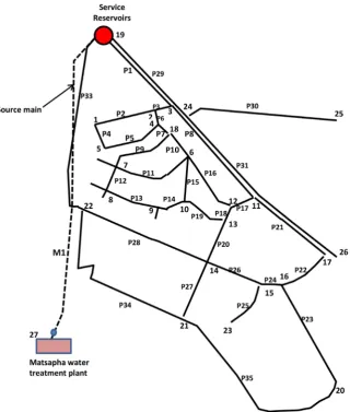
[image:7.595.212.533.324.702.2]This research study was conducted within the Matsapha town water distribution network shown in Figure 1 that is mainly fed from the two storage tanks located on the upper side of the demand area from which water flows to supply points by gravity. The treated water is pumped from the Matsapha water treatment plant into the two storage reservoirs that are connected with each other and each of which having isolating valves for cleaning and maintenance purposes. The Matsapha water treatment plant takes raw water from a river source and em-ploys conventional treatment technology with units consisting of screening, ae-ration, coagulation, flocculation, settlement, rapid sand filtration and finally disinfection using gas chlorination system. The water is pumped directly to the two service reservoirs after treatment. The average daily flow from the source into the network is 5.64 Million liters per day.
DOI: 10.4236/jwarp.2019.111003 44 Journal of Water Resource and Protection The water network map drawn with AutoCAD software was imported into the EPANET platform and the information required for analysis were digitized based on the map. The network consisted of a pump located at the source treat-ment works, the two water storage tanks and a pipe network consisting of 36 pipes and 28 nodes. The total length of the pipes in the network is 27.3 km. The hydraulic time step used for analysis was one hour. The chlorine bulk decay coefficient was determined for several initial chlorine concentrations using la-boratory bottle decay test. Since the bulk chlorine decay rate coefficient varies inversely with the initial chlorine used, a second order chlorine decay model was found to adequately model the relationship between the bulk decay rate coeffi-cient and the initial chlorine concentration. Accordingly, different bulk decay rates were calculated using the formula based on experimentally determined second order decay model which vary with the initial chlorine. Therefore, for each initial chlorine concentration used in the EPANET program, the corres-ponding value of bulk decay rate so calculated was used.
The wall decay coefficient was determined using field testing method by mea-suring the chlorine residual at the source after treatment and at four points within the distribution system using mobile Chlorimeter instrument. A trial and error procedure was used to determine the wall decay coefficient in which dif-ferent wall decay coefficient values were assumed and the extended period EPANET hydraulic simulations were carried out. After the run, the chlorine re-sidual values obtained were compared with the field determined values. The op-timum value of the wall decay coefficient was determined using least square method as the value with the minimum total least square error. For determining chlorine residuals in samples of water used for the bottle test which was used for the purpose of determining the bulk decay rates, Iodometric titration was used. The procedure used was according to the Standard Methods for the Examination of Water and Wastewater [30].
3. Results and Discussion
3.1. Second Order Modeling of Bulk Chlorine Decay Rate with the
Initial Chlorine Dose
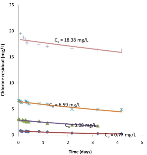
The residual chlorine values measured at different times for given initial chlorine used in the bottle test are plotted in Figure 2. The rate of reduction of chlorine residual with time is first order for a given initial chlorine concentration. Gener-ally the bulk decay rate decreases as expected with increase in the initial chlorine concentration. This trend is shown in Figure 2 for the four initial chlorine val-ues used in the test.
A second order model fit to the data shown in Figure 3 adequately describes the variation of the bulk decay rate with the initial chlorine. A regression analy-sis gives R2 = 0.99. Accordingly the model parameters were determined using
DOI: 10.4236/jwarp.2019.111003 45 Journal of Water Resource and Protection
Figure 2. Chlorine residual measurement at different times and
[image:9.595.259.498.370.512.2]initial chlorine dosages.
Figure 3. Second order regression model of reaction rate
con-stant with respect to initial concentration of chlorine.
Figure 4. Second order chlorine bulk decay modeling curve used
in the EPANET program.
0 5 10 15 20 25
0 1 2 3 4 5
Ch
lo
rin
e r
esi
du
al
(m
g/
L)
Time (days) Co= 18.38 mg/L
Co= 6.59 mg/L
Co= 3.08 mg/L
Co= 0.77 mg/L
0 10 20 30 40 50 60 70
0 5 10 15 20
1/
Kd
Initial chlorine, Comg/L R2= 0.99
Ko= 1.453
β= 0.580
0 0.1 0.2 0.3 0.4 0.5 0.6
0 2 4 6 8 10 12
Chlorine bulk decay coefficient
kd(day-1)
Initial chlorine residual at the source (mg/l) 𝐾_𝑑=0.252/(1+0.843
[image:9.595.258.499.558.694.2]DOI: 10.4236/jwarp.2019.111003 46 Journal of Water Resource and Protection
0
0.580 1 0.843
d
k
C =
+ (14)
3.2. Hydraulic and Chlorine Residual Modeling Using EPANET 2.0
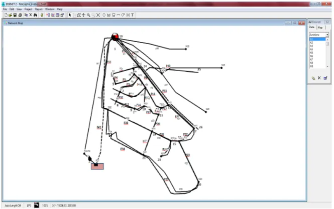
The Matsapha pipe network diagram available with AutoCAD drawing was im-ported and the required information was digitized using the toolbars available on EPANET 2.0 program. Figure 5 shows the drawing as digitized on the EPANET program. Information on average nodal demand, pipe diameter, length, roughness coefficient, ground elevation, etc. as needed by the EPANET program was entered appropriately. Table 1 shows the pipe and node data. For the pur-pose of modeling using the EPANET program, the two storage tanks were con-verted to an equivalent single storage tank having the same volume of water and the same height.For extended period simulation of the network, the time series flow data available for the treated water entering the distribution system was used. The diurnal variation in flow was divided into six time periods each of which had duration of four hours. The peak factor to be used for the extended period anal-ysis was worked out and is shown in Figure 6 as used in the EPANET program.
The chlorine residual model for variable decay rate was carried out by calcu-lating the variable decay rate corresponding to the initial chlorine entered into the EPANET program. Equation (14) stated above was used for such calculation.
3.3. Determination of Wall Decay Rate
[image:10.595.208.541.497.706.2]The pipe wall decay coefficient was determined using a trial and error procedure by assuming different wall decay rate values and running the EPANET water quality model and determining the chlorine residual at different points in the distribution system. The first order reaction rate has been used for modeling the
DOI: 10.4236/jwarp.2019.111003 47 Journal of Water Resource and Protection
Figure 6. Nodal flow pattern used in the extended period analysis.
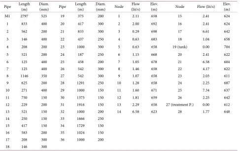
Table 1. The Matsapha network pipe and nodal demand data.
Pipe Length (m) Diam. (mm) Pipe Length (m) Diam. (mm) Node (lit/s) Flow Elev. (m) Node Flow (lit/s) Elev. (m) M1 2797 525 19 375 200 1 2.11 658 15 2.41 624
1 833 400 20 417 300 2 2.00 692 16 2.41 624 2 562 200 21 833 300 3 0.29 698 17 6.61 642 3 146 400 22 437 250 4 0.63 683 18 1.04 658 4 208 200 23 1000 300 5 0.63 658 19 (tank) 0.00 704 5 521 200 24 187 250 6 1.15 668 20 2.41 622 6 125 400 25 458 200 7 1.05 678 21 6.58 604 7 125 400 26 542 300 8 1.46 658 22 4.17 622 8 1146 350 27 542 300 9 1.07 658 23 2.03 611 9 625 200 28 1291 250 10 1.28 658 24 2.25 687 10 271 400 29 1000 150 11 1.60 671 25 7.34 637 11 750 150 30 1375 150 12 1.81 659 26 2.25 642 12 229 200 31 1916 150 13 2.29 658 27 (treatment P.) 0.00 612 13 521 150 32 1000 200 14 6.58 623 28 1.77 648 14 250 150 33 1666 250
15 417 150 34 1729 150 16 583 200 35 1024 150 17 208 300 36 1000 200 18 146 300
[image:11.595.56.544.303.609.2]DOI: 10.4236/jwarp.2019.111003 48 Journal of Water Resource and Protection
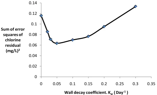
Figure 7. Plot of sum of error squares of chlorine residual plotted
against wall decay coefficient used in the EPANET model using four points selected from the network.
In order to identify sampling points for analysis, extended period simulation was run for a period of 288 hours. Figure 8 shows the plot of water age at the four sampling points selected afterwards. Sampling point at Spintex (Node 20) has the longest water age as it is located furthest from the service reservoir in the network. The other three points included SEC (Node 21) Old Airport (Node 24) and Tubungu (Node 25).
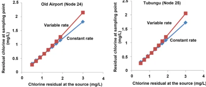
Comparison of chlorine residual modeling between constant and variable de-cay rates was made by running the EPANET simulation for the two alternate models. Figure 9 and Figure 10 show the model outputs of chlorine residual among the four stations. In general the constant rate decay model tends to un-derestimate the chlorine residual potentially leading to overdosing of chlorine at the source. The implication of this difference is that second order decay rate modeling results in lesser initial chlorine dosage compared to the constant rate in order to maintain the desired chlorine residual in the distribution system.
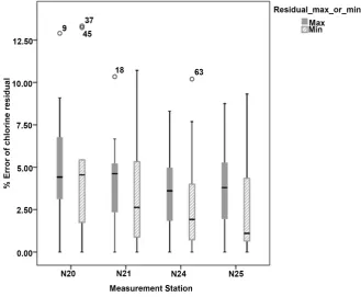
Figure 11 shows the percentage errors between the two alternate models for both the maximum and minimum chlorine residuals reported in the extended period simulation. The error varies with the distance from the network. Node 20 (Spintex) has the highest error as it is located longest distance followed by SEC (Node 21), Tubungu (N25) and Old airport (N24) in that order. In general, the error varies within ± 15%. This error can be eliminated through variable rate modeling resulting in saving of the cost of chlorine. In addition, higher dosing results in problems of taste and odour as well as formation of disinfection by-products that pose danger to human health. The use of variable rate model-ing in programs such as the EPANET, therefore, reduces the effects of excess chlorination at the source.
4. Conclusions
Modeling of chlorine residuals in water distribution systems is an important ex-ercise in the management and monitoring of chlorine dosages at the source and
0 0.02 0.04 0.06 0.08 0.1 0.12 0.14
0 0.05 0.1 0.15 0.2 0.25 0.3 0.35
Sum of error squares of
chlorine residual (mg/L)2
DOI: 10.4236/jwarp.2019.111003 49 Journal of Water Resource and Protection
Figure 8. EPANET extended period simulation of water age among the four sampling
[image:13.595.209.533.307.431.2]points within Matsapha network.
Figure 9. Residual chlorine at Spintex (Node 20) and SEC (N21) showing EPANET
out-put using two alternate models.
Figure 10. Residual chlorine at Old Airport (Node 24) and Tubungu (Node 25) showing
EPANET output using two alternate models.
the resulting residuals within water distribution systems. At present, the chlorine dosage within the Matsapha water network is managed through periodic check-ing of the residuals at different points and adjustcheck-ing the dosages at the source accordingly. Such procedure is cumbersome and requires constant monitoring
0 10 20 30 40 50 60 70
0 50 100 150 200 250 300 350
W
at
er a
ge
(h
r)
EPANET extended simulation period (hr)
Spintex (N20): Max = 61 hr
SEC (N21): Max = 51 hr
[image:13.595.208.537.480.619.2]DOI: 10.4236/jwarp.2019.111003 50 Journal of Water Resource and Protection
Figure 11. Percentage error of chlorine residual between constant and variable decay rate
models.
of the chlorine dosage and residuals within the network. EPANET modeling of chlorine residual using variable rate modeling gives more accurate results com-pared with the constant decay rate modeling. Constant decay rate modeling tends to underestimate chlorine residual, hence prompting chlorine over dosages at the source. By contrast, the variable decay rate model, as shown in this paper, enables saving of chlorine and reduction of the instances of excess chlorine re-siduals in the distribution system with the associated side effects.
It is suggested that such variable chlorine decay rate model be incorporated through EPANET extension programs in order to avoid hand calculation of the decay rate corresponding to the initial chlorine dosage used. In addition, several other water quality factors, such as dissolved organic matter, temperature, etc., can be incorporated into the variable decay rate model and be provided as ex-tension to the EPANET program.
Water distribution network management such as the Matsapha network should be encouraged to adopt process based models in order to properly manage chlo-rine residuals in the distribution systems, thereby avoiding instances of un-der-chlorination as well as over-chlorination with the associated dangers.
Acknowledgements
DOI: 10.4236/jwarp.2019.111003 51 Journal of Water Resource and Protection
Conflicts of Interest
The authors declare no conflicts of interest regarding the publication of this pa-per.
References
[1] Robescu, D., Jivan, N. and Robescu, D. (2008) Modeling Chlorine Decay in Drink-ing Water Mains. Environmental EngineerDrink-ing and Management Journal, 7, 737-741. https://doi.org/10.30638/eemj.2008.099
[2] White, G.C. (1972) Handbook of Chlorination. Van Nostrand Reinhold Company, New York, NY.
[3] EPA-Environmental Protection Agency (1974) New Orleans Area Water Supply Study. Lower Mississippi River Facility, Slidell.
[4] Vhutshilo, A., Madzivhandila, E. and Chirwa, M.N. (2017) Modeling Chlorine De-cay in Drinking Water Distribution Systems Using Aquasim. Chemical Engineering Transactions, 57, 1111-1116.
[5] Barakat, M.A., Tseng, J.M. and Huang, C.P. (2005) Hydrogen Peroxide-Assisted Photo Catalytic Oxidation of Phenolic Compounds. Applied Catalysis B: Environ-mental, 59, 99-104. https://doi.org/10.1016/j.apcatb.2005.01.004
[6] Gibbs, M.S., Morgana, N., Maiera, H.R., Dandya, G.C., Holmesb, M. and Nixon, J.B. (2006) Use of Artificial Neural Networks for Modeling Chlorine Residuals in Water Distribution Systems. Mathematical and Computer Modeling, 44, 485-498. https://doi.org/10.1016/j.mcm.2006.01.007
[7] Jones, S. and Marseden, P. (2017) Formation of DBPS during Booster Chlorination. Defra Project WT1291. Cranfield Water Science Institute, Cranfield University, Cranfield.
[8] Lebel, G.L., Benoit, F.M. and Williams, D.T. (1997) A One-Year Survey of Haloge-nated Disinfection By-Products in the Distribution System of Treatment Plants Us-ing Three Different Disinfection Processes. Chemosphere, 34, 2301-2317. https://doi.org/10.1016/S0045-6535(97)00042-8
[9] Williams, D.T., Lebel, G.L. and Benoit, F.M. (1997) Disinfection By-Products in Canadian Drinking Water. Chemosphere, 34, 299-316.
https://doi.org/10.1016/S0045-6535(96)00378-5
[10] Singer, P.C., Obolensky, A. and Greiner, A. (1995) DBPs in Chlorinated North Car-olina Drinking Waters. Journal of the American Water Works Association, 87, 83-92. https://doi.org/10.1002/j.1551-8833.1995.tb06437.x
[11] Williams, S.L., Rindfleisch, D.F. and Williams, R.L. (1995) Dead End on Haloacetic Acids (HAA). Proceedings of the AWWA Water Quality Technology Conference, San Francisco, 6-10 November 1994.
[12] Rodriguez, M.J., West, J.R., Powell, J. and Sérodes, J.B. (1997) Application of Two Approaches to Model Chlorine Residuals in Severn Trent Water Ltd (STW) Distri-bution Systems. Water Science and Technology, 36, 317-324.
https://doi.org/10.2166/wst.1997.0227
[13] Hua, F., West, J.R., Barker, R.A. and Forster, C.F. (1999) Modeling of Chlorine De-cay in Municipal Water System. Water Research, 33, 2735-2746.
https://doi.org/10.1016/S0043-1354(98)00519-3
Ini-DOI: 10.4236/jwarp.2019.111003 52 Journal of Water Resource and Protection tial Chlorine Concentration, TOC, Iron and Temperature When Modeling Chlorine Decay in Water Supply. Journal of Water Supply: Research and Technology, 53, 453-467. https://doi.org/10.2166/aqua.2004.0036
[16] Powell, J.C., Hallam, N.B., West, J.R., Forster, C.F. and Simms, J. (2000) Factors Which Control Bulk Chlorine Decay Rates. Water Research, 34, 117-126.
https://doi.org/10.1016/S0043-1354(99)00097-4
[17] Weber Jr., W.J. (1972) Physico-Chemical Processes for Water Quality Control. John Wiley and Sons, Inc., New York.
[18] Murphy, S.B. (1985) Modeling Chlorine Concentrations in Municipal Water Sys-tems. M.Sc. Thesis, Montana State University, Bozeman.
[19] Rossman, L.A., Clark, R.M. and Grayman, W.M. (1994) Modeling Chlorine Resi-duals in Drinking Water Distribution Systems. Journal of Environmental Engi-neering, 120, 803-820.https://doi.org/10.1061/(ASCE)0733-9372(1994)120:4(803) [20] Mayer, S.H., Powell, R.S. and Woodward, C.A. (2000) Calibration and Comparison
of Chlorine Decay Models for a Test Water Distribution System. Journal of Water Research, 34, 2301-2309.https://doi.org/10.1016/S0043-1354(99)00413-3
[21] Rossman, L.A., Uber, J.G. and Frayman, W.M. (1995) Modeling Disinfectant Resi-duals in Drinking Water Storage Tanks. Journal of Environmental Engineering, 121, 752-755.https://doi.org/10.1061/(ASCE)0733-9372(1995)121:10(752)
[22] HDR Engineering, Inc. (2001) Water Quality Control in Distribution Systems. In: Handbook of Public Water Systems, Wiley, Hoboken, 2nd Edition, 722-740. [23] Mohamed, A., Bensoltane, M.A., Zeghadnia, A.L., Djemili, L., Gheid, A. and
Djeb-bar, Y. (2018) Enhancement of the Free Residual Chlorine Concentration at the Ends of the Water Supply Network: Case Study of Souk Ahras City—Algeria. Jour-nal of Water and Land Development, 38, 3-9.
https://doi.org/10.2478/jwld-2018-0036
[24] Haider, H., Haydar, S., Sajid, M., Tesfamariam, S. and Sadiq, R. (2015) Framework for Optimizing Chlorine Dose in Small- to Medium-Sized Water Distribution Sys-tems: A Case of a Residential Neighborhood in Lahore, Pakistan. Water SA, 41, 614-623.https://doi.org/10.4314/wsa.v41i5.4
[25] Foong, Y.C., Ghazaly, M.D. and Othman, F. (2004) Modeling of Chlorine Residual in the Water Distribution Network at Bukit Tunku, Kuala Lampur. Malaysian Journal of Science, 23, 193-201.
[26] Clark, R.M. (1998) Chlorine Demand and THM Formation Kinetics: A Second-Order Model. Journal of Environmental Engineering, 124, 16-24.
https://doi.org/10.1061/(ASCE)0733-9372(1998)124:1(16)
[27] Kastl, G.J., Fisher, I.H. and Jegatheesan, V. (1999) Evaluation of Chlorine Decay Kinetics Expressions for Drinking Water Distribution Systems Modeling. Journal of Water Supply: Research and Technology Aqua, 48, 219-226.
https://doi.org/10.2166/aqua.1999.0024
[28] Fisher, I., Kast, G. and Sathasivan, A. (2011) Evaluation of Suitable Chlorine Bulk-Decay Models for Water Distribution Systems. Water Research, 45, 4896-4908. https://doi.org/10.1016/j.watres.2011.06.032
[29] Shang, F., Uber, J.G. and Rossman, L.A. (2008) Modeling Reaction and Transport of Multiple Species in Water Distribution Systems. Environmental Science & Tech-nology, 42, 808-814.https://doi.org/10.1021/es072011z