An Inventory Model for Ramp Type Demand with Two Level Trade Credit Financing Linked to Order Quantity

ISSN Online: 2329-3292 ISSN Print: 2329-3284

DOI: 10.4236/ojbm.2019.72029 Mar. 7, 2019 427 Open Journal of Business and Management

An Inventory Model for Ramp-Type Demand

with Two-Level Trade Credit Financing Linked

to Order Quantity

Hui-Ling Yang

Department of Computer Science and Information Engineering, Hungkuang University, Taiwan

Abstract

In the traditional economic order quantity (EOQ) model, it is assumed that the demand rate is constant. Thereafter, many researchers developed inven-tory model with time-varying demand to reflect sales in different phases of product life cycle in the market. However, in practice, especially for fashiona-ble and high-tech product, the demand rate during the growth stages of its life cycle increases significantly with linear or exponential in the growth stage and then gradually stabilizes, and remains near constant in the maturity stage. It can be taken a ramp-type demand rate into account. Furthermore, in today’s supply chain, a supplier usually offers a permissible delay in payment to retailers to encourage them to buy more products, and a retailer in turn provides a downstream trade-credit period to its customers. Therefore, this paper focus on 1) ramp-type demand rate and 2) the upstream and down-stream trade credit financing linked to order quantity for retailer is consi-dered. The objective is to find the optimal replenishment cycle and order quantity to keep the total relevant cost per unit time as minimum as possible. The study shows that in each case discussed, the optimal solution not only exists but also is unique. Numerical examples are provided to illustrate the proposed model. Finally, some relevant managerial insights based on the re-sults are characterized.

Keywords

Ramp-Type Demand, Two-Level, Trade Credit, Finance, Order Quantity

1. Introduction

1.1. Inventory Models with Ramp-Type Demand Rate

In present, high-tech manufacturing is the backbone to the Taiwan economy.

How to cite this paper: Yang, H.-L. (2019) An Inventory Model for Ramp-Type De-mand with Two-Level Trade Credit Fi-nancing Linked to Order Quantity. Open Journal of Business and Management, 7, 427-446.

https://doi.org/10.4236/ojbm.2019.72029

Received: January 31, 2019 Accepted: March 4, 2019 Published: March 7, 2019

Copyright © 2019 by author(s) and Scientific Research Publishing Inc. This work is licensed under the Creative Commons Attribution International License (CC BY 4.0).

DOI: 10.4236/ojbm.2019.72029 428 Open Journal of Business and Management

model with ramp type demand rate in which time dependent deterioration rate and shortages were considered. Agrawal et al. [3] provided an inventory model with deteriorating items, ramp-type demand and partially backlogged shortages for a two-warehouse system. Other related research articles on this field can be found in Deng [4], Deng et al. [5], Panda et al. [6] [7], Skouri et al. [8] [9] and their references.

1.2. Inventory Models with Permissible Delay in Payment

The traditional inventory economic order quantity (EOQ) model assumes that a buyer must pay for items immediately after receiving them. However, to stimu-late sales quantity a supplier often offers a retailer a permissible delay in pay-ment. Thus, to offer a certain fixed credit period for his/her retailer is an alterna-tive incenalterna-tive policy to quantity discount. In early research work, Goyal [10] de-veloped an EOQ model under conditions of permissible delay in payments, and ignored the difference between the selling price and the purchase cost. Shah [11]

considered a stochastic inventory model when delays in payments are permissi-ble. Aggarwal and Jaggi [12] extended Goyal’s model to consider the deteriorat-ing items. Jamal et al. [13] further generalized Aggarwal and Jaggi’s model to al-low for shortages. Teng [14] amended Goyal’s model by considering the differ-ence between unit price and unit cost, and found that it makes economic sense for a well-established buyer to order less quantity and take the benefits of the permissible delay more frequently. Skouri et al. [15] proposed an inventory model with ramp type demand rate under permissible delay in payment. Teng et al. [16] established an economic order quantity model with trade credit financ-ing for non-decreasfinanc-ing demand. Similarly, there are also many related articles published in such field with different practical consideration.

1.3. Inventory Models with Two-Level Trade Credit

Huang [17] extended Goyal’s model to develop an EOQ model in which the

supplier offers the retailer a permissible delay period (i.e., an upstream trade credit), and the retailer in turn provides a trade credit period (i.e., a downstream trade credit) to its customers. Teng and Goyal [18] complemented the short-coming of Huang’s model and proposed a generalized formulation. Teng et al.

DOI: 10.4236/ojbm.2019.72029 429 Open Journal of Business and Management

credit decision for time-varying deteriorating items with up-stream and down- stream trade credit financing by discounted cash flow analysis. Shah [22] pro-vided a three-layered integrated inventory model for deteriorating items with quadratic demand and two-level trade credit financing. Rameswari and Uthaya-kumar [23] proposed an integrated inventory model for deteriorating items with price-dependent demand under two-level trade credit policy. Several related ar-ticles can be found in Goyal et al. [24], Huang and Hsu [25], Min et al. [26] and their references.

1.4. Inventory Models with Trade Credit Linked to Order Quantity

Sometimes, to encourage more sales, supplier offer retailers a trade credit period with conditional permission, if a retailer orders more than a predetermined quan-tity. Chang et al. [27] developed an EOQ model for deteriorating items under sup-plier credits linked to ordering quantity. Chung and Liao [28] provided lot-sizing decisions under trade credit depending on the ordering quantity. Ouyang et al. [29]

proposed an economic order quantity for deteriorating items with partially per-missible delay in payments linked to order quantity. Kreng and Tan [30] proposed an inventory model under two levels of trade credit depending on the order quan-tity. Teng et al. [31] provided an inventory model for increasing demand under two levels of trade credit linked to order quantity, Recently, Sash and Carde-nas-Barrón [32] provided an inventory model which is a retailer’s decision for dering and credit policies with deteriorating items when a supplier offers or-der-linked credit or cash discount. Ting [33] provided some comments on the EOQ model for deteriorating items with conditional trade credit linked to order quantity. Similarly, other related research articles can be found in their references.

In contrast to the above papers mentioned, this paper is extended in the fol-lowing two ways: 1) a constant demand (or increasing demand) is extended to a

ramp-type demand function, in which the demand increases linearly and then stays constant at the end, and 2) the supplier provides its retailer with a per-missible delay link to order quantity while the retailer also offers a downstream trade credit period to its customers. We establish several fundamental theoretical results and obtain its optimal solution. We then provide several numerical ex-amples to illustrate the proposed model and present some important and rele-vant managerial insights.

The rest of the paper is structured as follows. Section2 introduces the notation and assumption needed to develop the proposed inventory model. Section 3 for-mulates the model. Section 4 discusses some theoretical results and provides an algorithm to find the optimal solutions. Section 5 provides numerical examples to illustrate the proposed model. Section 6 concludes the results and presents some managerial insights. Further, provides some future research directions.

2. Notation and Assumptions

follow-DOI: 10.4236/ojbm.2019.72029 430 Open Journal of Business and Management i.e.,

( )

( )

_{( )}

,

,

f t t D t

f t

µ

µ

µ

< 

=  _≥

 , where f t

( )

= +a bt, a>0, b>0.

d

Q = the minimum order quantity at which the delay is permitted by the

supplier.

d

T = the time interval that Qd units are depleted to zero due to demand.

M = the retailer’s upstream credit period offered by supplier in years.

N = the retailer’s downstream credit period offered to its buyers in years.

T = the length of replenishment cycle in years.

Q = the order quantity.

A = the replenishment cost per order.

h = the holding cost per unit per unit of time excluding interest charge.

p= the unit selling price.

c = the unit purchasing cost.

e

I = the interest earned per dollar per year by the retailer.

p

I = the interest paid per dollar per year by the retailer.

( )

I t = the inventory level at time t.

( )

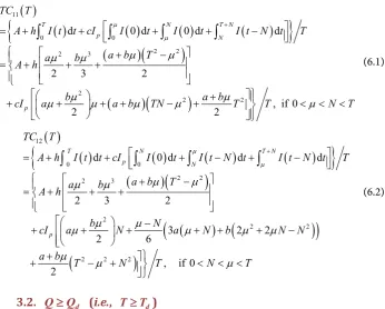
ij

TC T = the total relevant cost per unit time for Case i and subcase j, 1,2,3,4

i= and j=1,2 _{or 3, which is a function of T.}

*

ij

T = the optimal replenishment cycle time of TC Tij

( )

for Case i and

sub-case j, i=1,2,3,4 and j=1,2 _{or 3. (i.e., T}*_).

*

ij

Q = the optimal order quantity for Case i and subcase j, i=1,2,3,4 _and 1,2

j= _{or 3. (i.e., Q}*_).

2.2. Assumptions

Next, the following assumptions are made to establish the mathematical inven-tory model.

1) Replenishment rate is instantaneous. 2) Shortages are not allowed to occur.

3) In today’s global competition, many retailers have no pricing power. As a result, the selling price is hardly changed for many retailers. In addition, to avoid lasting price competition, we may assume without loss of generality that the selling price is constant in today’s global competition and low inflation envi-ronment.

4) The objective here is to minimize the total relevant cost per unit of time until the demand is no longer increasing.

DOI: 10.4236/ojbm.2019.72029 431 Open Journal of Business and Management

account from time N to M. At the end of the permissible delay, the buyer pays off all units sold by time M N− , uses uncollected and unsold items as collateral to apply for a loan, and pays the bank a certain amount of money periodically until the loan is paid off at time T N+ .

3. Mathematical Formulation

Based on the above assumptions, the inventory system here is as follows. At the beginning (i.e., at time t = 0), the retailer orders and receives Q units of a single product from the supplier. The inventory level is depleted gradually in the in-terval [0, T] due to increasing demand from customers. At time t = T, the in-ventory level reaches zero. Hence, the inin-ventory level at time t, I(t), can be de-scribed by the following differential equation:

( )

_{( )}

( )

_{( )}

d

, 0 d

d

, d

I t

f t t t

I t

f t T t

µ

µ µ

= − ≤ ≤

= − ≤ ≤

(1)

with the boundary condition I T

( )

=0. The solution to (1) is

( )

(

)

(

)

(

)(

)

(

)(

)

2 2 _{2 , 0}

,

I t a t b t a b T t

a b T t t T

µ µ µ µ µ

µ µ

= − + − + + − ≤ ≤

= + − ≤ ≤

(2)

Thus, the retailer’s order quantity per cycle is

( )

₀ 2 ₂

(

)(

)

Q I= =a

µ

+b

µ

+ a b+

µ

T−

µ

₍₃₎

From Equation (3), we can obtain the time interval Td by using the following

equations:

(

)(

)

2 ₂

d d

Q =a

µ

+b

µ

+ a b+

µ

T −

µ

(4)

Next, based on whether the order quantity larger than the predetermined quantity or not, we have the following two cases: 1) T T< d 2) T T≥ d.

3.1.

Q Q

<

_d

(

i.e.

,

T T

<

_d

)

In this case, the retailer’s order quantity is less than Qd. Hence, the permissible

delay in payment is not allowed (i.e., M = 0). Meanwhile, the retailer offers a permissible delay of N to its buyers. Consequently, the retailer must fiancé all items ordered at time 0, and start to payoff the loan after time N. For details, please see Figure 1. Thus, the interest paid by the retailer is as follows. There are two cases to be discussed. 1) 0<µ<N T< ₂₎ 0<N<µ<T

( )

(

)

( )

( )

(

)

( )

(

)

(

)

0

0

0

0 d d

0 d 0 d d , if 0

0 d d d , if 0

N T N

p _N

N T N

p _N

N T N

p _N

cI I t I t N t

cI I t I t I t N t N T

cI I t I t N t I t N t N T

µ

µ µ

µ

µ

µ

+

+

+

 _{+ −} 

 

 

  _{+ + −}  _{< < <}

 

  

= 

 

 _ + − + − _ < < <

 



∫

∫

∫

∫

∫

∫

∫

∫

(5)

[image:6.595.192.539.208.486.2]

DOI: 10.4236/ojbm.2019.72029 432 Open Journal of Business and Management Figure 1. Graphical representation for T T< d.

( )

( )

( )

( )

(

)

{

}

(

)

(

)

(

)

(

)

11 0 0 2 2 2 3 2 2 2

d 0 d 0 d d

2 3 2

, if 0

2 2

T N T N

p _N

p TC T

A h I t t cI I t I t I t N t T

a b T

a b

A h

b a b

cI a a b TN T T N T

µ

µ

µ µ

µ µ

µ µ

µ µ µ µ µ

+   = + + _ + + − _     _{+ −}   _{ } =_ + + +    _{ }     + 

+ _ + _ + + − + _ < < <

    

∫

∫

∫

∫

(6.1)

( )

( )

( )

(

)

(

)

{

}

(

)

(

)

(

)

(

)

(

)

(

)

12 0 0 2 2 2 3 2 2 2

2 2 2

d 0 d d d

2 3 2

3 2 2

2 6

, if 0 2

T N T N

p _N

p

TC T

A h I t t cI I t I t N t I t N t T a b T

a b A h

b N

cI a N a N b N N a b T N T N T

µ

µ

µ µ

µ µ

µ µ

µ µ µ µ

µ _{µ µ}

+   = + + _ + − + − _     _{+ −}   _{ } =_ + + +    _{ }    − + _ + _ + + + + −    + 

+ − + _ < < <

∫

∫

∫

∫

(6.2)

3.2.

Q Q

≥

_d

(

i.e.

,

T T

≥

_d

)

In this case, based on the supplier’s trade credit M, and the last customer’s pay-ment time T + N, we discuss the following three cases: 1) 0<M N< 2)

M N≥ _and M T N≤ + ₃₎ M N≥ _and M T N> + _.

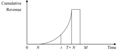
3.2.1.The Case of 0 M N< <

Since 0<M N< , there is no interest earned for the retailer. In addition, the retailer has to finance all items ordered after time M at an interest charged Ip

per dollar per year, and start to pay off the loan after time N as shown in Figure 2. Consequently, the interest charged is given by

( )

(

)

( )

(

)

( )

( )

(

)

( )

(

)

(

)

0 d d

0 d d , if 0

0 d 0 d d , if 0

0 d d d , if 0

N T N

p _{M N}

N T N

p _{M N}

N T N

p _{M N}

N T N

p _{M N}

cI I t I t N t

cI I t I t N t M N T cI I t I t I t N t M N T cI I t I t N t I t N t M

µ µ µ µ µ µ + + + +  _{+ −}     

 _{+ −}  _{< < < <}

 

 

 

= _ + + − _ < < < <

 

 _{+ − + −}  _<

 

 

∫

∫

∫

∫

∫

∫

∫

∫

∫

∫

N µ T

    

 < < <



[image:7.595.260.486.70.189.2]

DOI: 10.4236/ojbm.2019.72029 433 Open Journal of Business and Management Figure 2. Graphical representation for T T≥ d and M N< .

Hence, the retailer’s total relevant cost per unit time is

( )

( )

( )

(

)

{

}

(

)

(

)

(

) (

)

21 0 2 2 2 3 2

d 0 d d

2 3 2

, if 0 2

T N T N

p _{M N}

p

TC T

A h I t t cI I t I t N t T a b T

a b A h

T

cI a b T N M T M N T

µ µ µ µ µ µ +   = + + _ + − _     + −   _{ } = + + +    _{ }    

+ + _ − + _ < < < <

  

∫

∫

∫

(8.1)

( )

( )

( )

( )

(

)

{

}

(

)

(

)

(

)

(

) (

)

(

)

22 0 2 2

2 3 2

2

d 0 d 0 d d

2 3 2 2

, if 0 2

T N T N

p _{M N}

p

TC T

A h I t t cI I t I t I t N t T a b T

a b b

A h cI a M

T

a b T N M M T M N T

µ

µ

µ

µ

µ

µ

_µ

µ

_µ

µ

µ

µ

µ

+   = + + _ + + − _   _{+ −}  _{ }  _{ } = + _ + + _+  +  −    _{ }       

+ +  − + − +  < < < <

  

∫

∫

∫

∫

(8.2)

( )

( )

( )

( )

(

)

{

}

(

)

(

)

(

)

(

)

(

)

(

)

(

)(

)

(

)

23 0 2 2

2 3 2

2 2

2

d 0 d 0 d d

2 3 2 2

3 2 2

6

2 2 , if 0

2

T N T N

p _{M N}

p

TC T

A h I t t cI I t I t I t N t T a b T

a b b

A h cI a N M

N a N b N N

a b _{T T N M N T M N T}

µ

µ

µ µ

µ µ _µ µ

µ _{µ µ µ}

µ _{µ µ µ}

+   = + + _ + + − _     + −  _{ }  _{ } = + + + +  +  −   _{ }  _{ }   − + + + + − + 

+ − + + − + _ < < < <

∫

∫

∫

∫

(8.3)

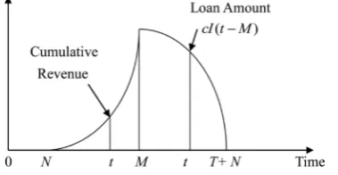
3.2.2. The Case of M≥ N and M T N≤ +

When M T N≤ + , the retailer cannot receive the last payment before the per-missible delay time M. As a result, the retailer must finance all items sold after time (M N− ) at time M, and pay off the loan until T + N at an interest rate of

p

[image:8.595.281.471.74.172.2]

DOI: 10.4236/ojbm.2019.72029 434 Open Journal of Business and Management Figure 3. Graphical representation for T T≥ d, 0<N M≤ and M T N≤ + .

(

)

( )

( )

( )

(

)

d

d d , if

d d d , if

T N p M

T N T p M t M

T N T

p M t M

cI I t M t

cI f v t M

cI µ f v v _µ f v t M

µ µ µ µ + + − + − −  _≤  =  + < 

∫

∫ ∫

∫

∫

∫

(9)

On the other hand, the retailer starts selling products at time 0, and receiving the money at time N. Consequently, the retailer accumulates sales revenue in an account that earns Ie per dollar per year starting from N through M as shown

in Figure 3. Therefore, the interest earned is given by

( )

( )

( )

(

)

( )

(

)

( )

(

)

0 0 0 d d

d d d , if

d d d d , if

M t N e N

M t N

e N

M N t N

e N N

pI f v v t

pI f v v f v t N

pI f v v f v N v f v t N

µ µ µ µ µ µ µ µ − − −  _{+ ≤}  = 

+ − + <

 

∫ ∫

∫ ∫

∫

∫ ∫

∫

∫

(10)

As a result, the retailer’s total relevant cost per unit time is

( )

{

( )

( )

( )

( )

(

)

}

(

)

(

)

(

)

(

)

(

)

(

) (

)(

) (

)

31 ₀ 0 2 2 2 3 2 2 2 2

d d d

d d d

2 3 2

2

2

, if 0 2

T T N T

p M t M

M t N

e N

p e

TC T A h I t t cI f v t

pI f v v f v t T

a b T

a b

A h

b

cI a b T M N pI a M N

M N

a b M N M N T N M

µ µ µ µ µ µ µ µ µ µ µ

µ µ µ

+ − − = + + − +   + −   _{ } =_ + + +    _{ }      + + _ − − _ − _ +  −       ₋  _   

+ + − − − − _ < ≤ <

 _  

∫

∫ ∫

∫ ∫

∫

(11.1)

( )

{

( )

( )

( )

(

)

( )

(

)

}

(

)

(

)

(

)

(

)

(

)

(

)(

)

(

) (

)(

) (

)

32 ₀ 0 2 2 2 3 2 2 2 2

d d d

d d d d

2

2 3 2

2

2

T T N T

p M t M

M N t N

e N N

p

e

TC T A h I t t cI f v t

pI f v v f v N v f v t T

a b T

a b

A h cI a b T M N

b

pI a M N bN N M N

M N

a b M N M N

µ

µ

µ

µ

µ µ

µ µ _µ

µ µ µ µ µ + − − = + + − + − +   + −   _{   } =_ + + + + + _ − − _    _{ }    − _ +  − − − −       ₋  _    + + − − − − _  _  

∫

∫ ∫

∫ ∫

∫

∫

, if 0

T <N< <µ M



DOI: 10.4236/ojbm.2019.72029 435 Open Journal of Business and Management

( )

{

( )

(

( )

( )

)

( )

( )

(

)

}

(

)

(

)

(

)

(

)

(

) (

)

(

)

(

)(

)

(

)

33 ₀ 0 2 2 2 3 3 2 2 2 2

d d d d

d d d

2 3 2

2 2 3

2

T T N T

p M t M

M N t N

e N N

p

e

TC T A h I t t cI f v v f v t

pI f v v f v t T

a b T

a b

A h

T N M

a b

cI M T N T N M

b

pI a M N bN N M N

a b µ µ µ µ µ µ µ µ µ µ

µ µ µ

µ µ µ µ + − − − − = + + + − +   + −   _{ } = + + +    _{ }    _{+ −}     + − + − − + _ + − − _  _{ }    − _ + _ − − − −    + +

∫

∫

∫

∫

∫ ∫

∫

(

)(

) (

)

2 , if 0

2 M N

M N µ M N  T N M µ

 ₋  _



 − − − −   < < <

 _

 _

(11.3)

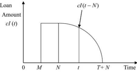
3.2.3. The Case of M≥ N and M T N> +

Since the order quantity is larger than or equal to Qd (due to Td ≤T ), the

re-tailer receives the permissible delay in payment. If T N M+ < _{, then the retailer} receives all payments from its customers by the time T + N which is before the permissible delay time M. Hence, the retailer has the money to pay the supplier at time M, and does not have the interest charges. In the meantime, the retailer rece-ives the revenue and deposits into a bank to earn interest as shown in Figure 4. The interest earned by the retailer is

( ) (

)

( )

( )

( )

( )

( )

(

)

( )

( )

(

)

( )

(

)

( )

0 0 0

0 d 0 d

d d 0 d

d d d 0 d , if

d d d d 0 d

T N M

e _{N T N}

T N t N M

e _{N T N}

T N t N M

e _{N T N}

T N N t N M

e _{N N T N}

pI I I t N t I t pI f v v t I t

pI f v v f v t I t N M

pI f v v f v N v f v t I t

µ µ µ µ

µ

µ

µ

+ + + − + + − + + − +  _{ − −  +}        = _ + _

 _{+ +}  _{< <}

    = + − + +

∫

∫

∫ ∫

∫

∫

∫

∫

∫

∫

∫

∫

∫

∫

, if N

µ

M

  

 

 _{ } < <

  



(12)

Hence, the retailer’s total relevant cost per unit time is

( )

{

( )

(

( )

( )

)

( )

}

(

)

(

)

(

)

(

) (

)(

)

41 _{0 0}

2 2

2 3 2

2

d d d d

0 d

2 3 2 2

, if 0 2

T T N t N

e _N

M T N

e

TC T A h I t t pI f v v f v t

I t T

a b T

a b b

A h pI a M N

T

a b T M N T N T N M

µ

µ µ

µ µ

µ µ _µ µ

µ µ µ

+ − +  = + − _ +  + _   + −  _{ }  _{ } =_ + + + − _ + _ −   _{ }  _{ }       

+ + _ − − − _ < < < + <

  

∫

∫

∫

∫

∫

(13.1)

( )

{

( )

(

( )

(

)

( )

)

( )

}

42 ₀ d ₀ d d

d d 0 d

T T N N

e _{N N}

t N M

T N

TC T A h I t t pI f v v f v N v

f v t I t T

[image:10.595.257.494.72.174.2]

DOI: 10.4236/ojbm.2019.72029 436 Open Journal of Business and Management Figure 4. Graphical representation for T T≥ d, 0<N M≤ and M T N> + .

(

)

(

)

(

)

(

)

(

) (

)(

)

2 2 2 3 2 2

2 3 2

2

, if 0 .

2 e

a b T

a b

A h

b

pI a M N bN N T

T

a b T M N T N T N M

µ µ

µ µ

µ

µ µ

µ µ µ

  + −   _{ } =_ + + +    _{ }    − _ + _ − − −        

+ + _ − − − _ < < < + <

  

(13.2)

4. Theoretical Results

To minimize the total relevant cost, taking the first and second order derivatives

of TC Tij

( )

, i=1,2,3,4, j=1,2 or 3 with respect to T and let

( )

dTC Tij dT =0, we obtain the following results.

(

)

(

)(

)

{

}

11 11 d ₀ d p

TC _{h a b T cI a b T N TC T}

T = + µ + + µ + − = , (14.1)

(

)

(

)

{

}

12 12 d ₀ d p

TC _{h a b T cI a b T TC T}

T = + µ + + µ − = , (14.2)

(

)

(

)

1 2 1 2 d 0 d d 0 d j j p TC T TC

h cI a b T

T ₌ = + + µ > , j=1,2. (15)

(

)

(

)(

)

{

}

2 2 d 0 d j p j TC

h a b T cI a b T N M TC T

T = + µ + + µ + − − = , j=1,2,3. (16)

(

)

(

)

2 2 2 2 d 0 d d 0 d j j p TC T TC

h cI a b T

T ₌ = + + µ > , j=1,2,3. (17)

(

)

(

)

{

}

3 3 d 0 d j p j TC

h cI a b T TC T

T = + + µ − = , j=1,2. (18.1)

(

)

(

)

(

)

(

)

33 2 2 33 d d 2 0 p

TC _{h a b T cI a M T N}

T

b _{T N M TC T}

µ µ µ   =_ + + + − −     + − + − _− _  =

(18.2)

(

)

(

)

3 2 3 2 d 0 d d 0 d j j p TC T TC

h cI a b T

DOI: 10.4236/ojbm.2019.72029 437 Open Journal of Business and Management

(

)

(

(

)

)

33 2

33

2 _d

0 d

d ₀

d TC p

T

TC _{h a b cI a b T N M T}

T ₌ = + µ − + + −  > . (19.2)

(

)

(

)(

)

{

}

41

41

d ₀

d e

TC _{h a b T pI a b M T N TC T}

T = + µ − + µ − − − = , (20.1)

(

)

(

) (

)(

)

{

}

42

42

d ₀

d e

TC _{h a b T pI bN N a b M T N TC T}

T = + µ − − −µ + + µ − − − = , (20.2)

(

)(

)

4

2 4 2

d 0 d

d

0

d j

j

e TC

T

TC

h pI a b T

T ₌ = + + µ > , j=1,2. (21)

Theorem 1. For each i, j, there exists a unique optimal cycle length Tij which

minimizes TCij, i=1, 2,3, 4, j=1,2 or 3.

Proof: See Appendix.

It is not easily to find the closed-form of T from the equation of each first de-rivative which is equal to zero. However, we can use numerical method to find the solution. From Theorem 1, we know that the solution minimizes the total relevant cost function is also a global minimum. By ensuring the solution satis-fies the condition in each case, the following theoretical result is obtained.

Corollary 1. For Q Q< d,

(a) if T11<Td and 0< <µ N T< 11, then T*=T11.

(b) if T12<Td and 0<N< <µ T12, then T*=T12

Corollary 2. For Q Q≥ d,

(a) 0<M N< ,

(i) if T21≥Td and 0< <µ M N T< < 21, then T*=T21.

(ii) if T22 ≥Td and 0<M< <µ N T< 22, then T*=T22.

(iii) if T23 ≥Td and 0<M N< < <µ T23, then T*=T23

(b) 0<N M≤ and M T N≤ + ,

(i) if T31≥Td and 0< ≤µ N M T< ≤ 31+N, then T*=T31.

(ii) if T32 ≥Td and 0<N < <µ M T≤ 32+N, then T*=T32.

(iii) if T33≥Td and 0<N M< < ≤µ T33+N, then T*=T33.

(c) 0<N M≤ _and M T N> +

(i) if T41≥Td and 0< <µ N T< 41+N M< , then T*=T41.

(ii) if T42 ≥Td _and 0<N < <µ T42+N M< , then T*=T42.

Summarizing the results in Corollary 1 and 2, we propose the following algo-rithm to find the optimal solution.

Algorithm

Step 0. Input parameter values. Step 0.1. By (4), calculate Td

Step 0.2. Compare the values of M and N. If M N< , then go to Step 1. Otherwise, go to Step 4.

Step 1. By (14.1), (14.2), (16), calculate T, let it be T11, T12, T21, T22, T23.

Step 2. Compare the values of Tij, i=1,2, j=1,2 or 3, and Td.

calcu-DOI: 10.4236/ojbm.2019.72029 438 Open Journal of Business and Management

calculate TC T22

( )

. Otherwise, set TC T22

( )

22 = ∞.

Step 2.5. If T23≥Td and 0<M N< < <µ T23, then T*=T23 and

calculate

( )

*

23

TC T . Otherwise, set TC T23

( )

23 = ∞.

Step 3. Set

( )

* _min

{

( )

_{1,2, 1,2 or 3}

}

ij ij

TC T = TC T i= j= , then *

ij

T =T is the optimal solution, for a certain i, j and stop.

Step 4. By (18.1), (18.2), (20.1), (20.2), calculate T, let it be T31, T32, T33, T41, 42

T .

Step 5. Compare the values of Tij, i=3,4, j=1,2 or 3, and Td.

Step 5.1. If T31≥Td and 0< ≤µ N M T< ≤ 31+N, then T*=T31

and calculate

( )

*

31

TC T . Otherwise, set TC T31

( )

31 = ∞.

Step 5.2. If T32≥Td and 0<N< <µ M T≤ 32+N , then T*=T32

and calculate

( )

*

32

TC T , Otherwise, set TC T32

( )

32 = ∞.

Step 5.3. If T33≥Td and 0<N M< < ≤µ T33+N, then T*=T33

and calculate

( )

*

33

TC T , Otherwise, set TC T33

( )

33 = ∞

Step 5.4. If T41≥Td and 0< <µ N T< 41+N M< , then

* 41

T =T .and calculate

( )

*

41

TC T . Otherwise, set

( )

41 41

TC T = ∞.

Step 5.5. If T42≥Td _and 0<N< <µ T42+N M< , then T*=T42

and calculate

( )

*

42

TC T . Otherwise, set TC T42

( )

42 = ∞.

Step 6. Set

( )

* _min

{

( )

_{3,4, 1,2 or 3}

}

ij ij

TC T = TC T i= j= _{, then} *

ij

T =T _{is the}

optimal solution, for a certain i, j and stop.

5. Numerical Examples

In this section, we provide two numerical examples to illustrate several distinct theoretical results for M > N and M < N. Let the demand rate f t

( )

=100 50+ t per year, A = $10 per order, h = $3/unit/year, c = $5/unit, p = $10/unit, Ip = 0.06/year, and Ie = 0.05/year.

5.1.

M

<

N

Let M = 1/12 years, and N = 1/6 years. 1) Let Qd =30 units.

Example 1.1. Let µ=0.1 years, we know that µ<N. By (4), we have 0.28810

d

T = _{years and by the above algorithm, we have}

11 0.23986, 12 0.24614, 21 0.23995, 22 0.23993, 23 0.23998

T = T = T = T = T = and

( )

11 11 88.36124

DOI: 10.4236/ojbm.2019.72029 439 Open Journal of Business and Management

( )

23 23

TC T = ∞. Since T11<Td and µ <N T< 11, by Corollary 1(a), we know

that the optimal solution is *

11 0.23986

T =T = _{years, and then}

( )

*

( )

11 11 88.36124

TC T =TC T = . Furthermore, by (3), we have

*

11 24.93522

Q =Q = _units.

Example 1.2. Let µ=0.2 years, we know that N<µ. By (4), we have 0.28182

d

T = _{years and by the above algorithm, we have}

11 0.23165, 12 0.24440, 21 0.23237, 22 0.23195, 23 0.23197

T = T = T = T = T = and

( )

11 11

TC T = ∞_, TC T₁₂

( )

₁₂ =88.71856_, TC T₂₁

( )

₂₁ = ∞_, TC T₂₂

( )

₂₂ = ∞_,

( )

23 23

TC T = ∞. Since T12<Td and N< <µ T12, by Corollary 1(b), we know

that the optimal solution is *

12 0.24440

T =T = _{years, and then}

( )

*

( )

12 12 88.71856

TC T =TC T = . By (3), we have *

12 25.88441

Q =Q = units.

2) Let Qd =20 units.

Example 1.3. Let µ=0.05 _{years, we know that} µ<M N< _{. By (4), we have} 0.19573

d

T = _{years and by the above algorithm, we have}

11 0.24311, 12 0.24632, 21 0.24312, 22 0.24313, 23 0.24324

T = T = T = T = T = and

( )

11 11

TC T = ∞_, TC T₁₂

( )

₁₂ = ∞_, TC T₂₁

( )

₂₁ =84.79927_, TC T₂₂

( )

₂₂ = ∞_,

( )

23 23

TC T = ∞. Since T21>Td and µ <M N T< < 21, by Corollary 2(a)(i), we

know that the optimal solution is *

21 0.24312

T =T = _{years, and then}

( )

*

( )

21 21 84.79927

TC T =TC T = . By (3), we have *

21 24.85773

Q =Q = units.

Example 1.4. Let µ=0.1 _{years, we know that} M < <µ N_{. By (4), we have}

0.19286 d

T = _{years and by the above algorithm, we have}

11 0.23986, 12 0.24614, 21 0.23995, 22 0.23993, 23 0.23998

T = T = T = T = T = and

( )

11 11

TC T = ∞, TC T12

( )

12 = ∞, TC T21

( )

21 = ∞, TC T22

( )

22 =85.76229,

( )

23 23

TC T = ∞_{. Since} T₂₂ >T_{d and} M< <µ N T< _{22, by Corollary 2(a)(ii), we} know that the optimal solution is *

22 0.24440

T =T = years, and then

( )

*

(

)

22 22 85.76229

TC T =TC TC = _{. By (3), we have} *

22 24.94312

Q =Q = _units.

Example 1.5. Let µ=0.2 _{years, we know that} M N< <µ_{. By (4), we have}

0.19091 d

T = _{years and by the above algorithm, we have}

11 0.23165, 12 0.24440, 21 0.23237, 22 0.23195, 23 0.23197

T = T = T = T = T = and

( )

11 11

TC T = ∞, TC T12

( )

12 = ∞, TC T21

( )

21 = ∞, TC T22

( )

22 = ∞,

( )

23 23 86.95530

TC T = .. Since T23>Td and M <N<µ<T23, by Corollary 2(a)

(iii), we know that the optimal solution is *

23 0.23197

T =T = years, and then

( )

*

( )

23 23 86.95530

TC T =TC T = . By (3), we have *

23 24.51676

Q =Q = units.

5.2.

M N

≥

DOI: 10.4236/ojbm.2019.72029 440 Open Journal of Business and Management

we know that the optimal solution is *

31 0.23967

T =T = years, and then

( )

*

( )

31 31 81.06808

TC T =TC T = . By (3), we have *

31 24.50358

Q =Q = units.

Example 2.2. Let µ=0.1 years, we know that N< <µ M. By (4), we have 0.19286

d

T = years and by the above algorithm, we have

31 0.23654, 32 0.23658, 33 0.25808, 41 0.23311, 42 0.23435

T = T = T = T = T = and

( )

31 31

TC T = ∞, TC T32

( )

32 =81.97423, TC T33

( )

33 = ∞, TC T41

( )

41 = ∞,

( )

42 42

TC T = ∞. Since T32>Td and N< <µ M T< 32+N, by Corollary 2(b)(ii),

we know that the optimal solution is *

32 0.23658

T =T = years, and then

( )

*

( )

32 32 81.97423

TC T =TC T = . By (3), we have *

32 24.59067

Q =Q = _units.

Example 2.3. Let µ=0.2 years, we know that N M< <µ. By (4), we have 0.19091

d

T = _{years and by the above algorithm, we have}

31 0.22922, 32 0.22946, 33 0.24603, 41 0.22611, 42 0.23447

T = T = T = T = T = and

( )

31 31

TC T = ∞_, TC T₃₂

( )

₃₂ = ∞_, TC T₃₃

( )

₃₃ =82.41147_, TC T₄₁

( )

₄₁ = ∞_,

( )

42 42

TC T = ∞. Since T32 >Td and N M< < <µ T33+N, by Corollary 2(b)

(iii), we know that the optimal solution is *

33 0.24603

T =T = _{years, and then}

( )

*

( )

33 33 82.41147

TC T =TC T = . By (3), we have *

33 26.06367

Q =Q = units.

2) Let M = 1/3 years, and N = 1/12 years.

Example 2.4. Let µ=0.05 years, we know that µ<N M< . By (4), we have 0.19573

d

T = _{years and by the above algorithm, we have}

31 0.20977, 32 0.20953, 33 0.22573, 41 0.23617, 42 0.23366

T = T = T = T = T = and

( )

31 31

TC T = ∞_, TC T₃₂

( )

₃₂ = ∞_, TC T₃₃

( )

₃₃ = ∞_, TC T₄₁

( )

₄₁ =71.91272_,

( )

42 42

TC T = ∞. Since T41>Td and µ <N T< 41+N M< , by Corollary 2(c)(i),

we know that the optimal solution is *

41 0.23617

T =T = _{years, and then}

( )

*

( )

41 41 71.91272

TC T =TC T = . By (3), we have *

41 24.14471

Q =Q = units.

Example 2.5. Let µ=0.1 years, we know that N< <µ M. By (4), we have 0.19286

d

T = _{years and by the above algorithm, we have}

31 0.20641, 32 0.20653, 33 0.21635, 41 0.23336, 42 0.23459

T = T = T = T = T = and

( )

31 31

TC T = ∞, TC T32

( )

32 = ∞, TC T33

( )

33 = ∞, TC T41

( )

41 = ∞,

( )

42 42 73.05178

TC T = _{. Since} T₄₂ >T_{d and} N< <µ T₄₂+N M< _{, by Corollary} 2(c)(ii), we know that the optimal solution is *

42 0.23459

DOI: 10.4236/ojbm.2019.72029 441 Open Journal of Business and Management

then

( )

*

( )

42 42 73.05178

TC T =TC T = . By (3), we have *

42 24.38186

Q =Q =

units.

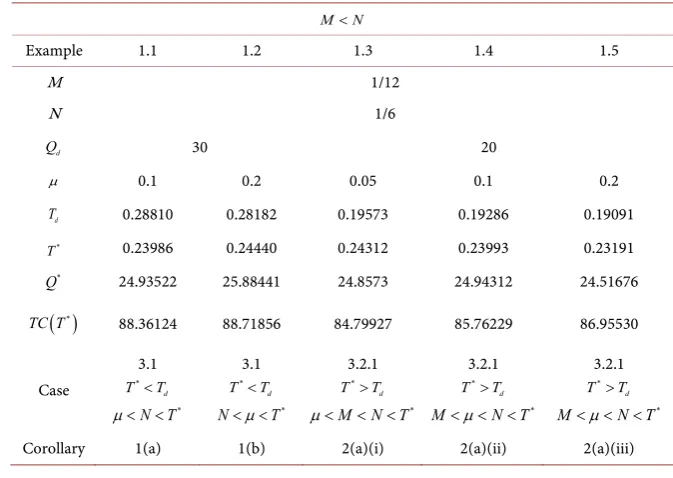
From Table 1, some managerial insights can be obtained. In the case of

M N< ,

a) The retailer’s total relevant cost _{TC T}

( )

* _{increases as the predetermined}

order quantity Qd increase, and the constant rate of a period time µ increase.

That is, if the predetermined order quantity (Qd) is larger and the period time

(µ) is longer, then the total relevant cost _{TC T}

( )

* _{for the retailer will be large.}

b) As the order quantity is less than the predetermined quantity, ( * d

T <T ), the optimal replenishment cycle _T* _{and the optimal order quantity Q}*

increase as the time point (µ) increases, while in the case, the order quantity is larger than the predetermined quantity ( *

d

T >T _{), the optimal replenishment cycle T}*

decreases as the time point (µ)increases.

In this case, if the upstream trade credit period is less than the downstream trade credit period, (M N< ), then the retailer need to pay more interest than earned, thus, the larger Qd, and µ will cause the larger total relevant cost.

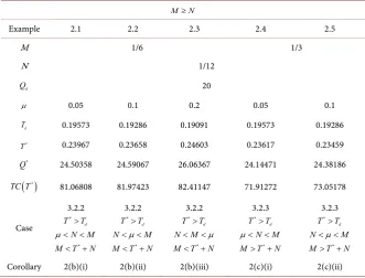
From Table 2, some managerial insights can be obtained. In the case of M N≥ , a) The retailer’s total relevant cost _{TC T}

( )

* _{and the optimal order quantity}

*

Q increase as the constant rate of a period time (µ) increases. That is, if the period time (µ) is longer, then it will cause the retailer’s total relevant cost and the optimal order quantity to be larger.

b) The retailer’s total relevant cost _{TC T}

( )

* _{decreases as the upstream trade}

[image:15.595.201.538.489.728.2]

credit period M increases, since the retailer may earn more interest than paid. c) The larger the difference of M N− _{,(i.e., the shorter downstream trade} credit period, and the longer upstream trade credit period), the less the retailer’s total relevant cost is. That is, it’s more profitable for the retailer.

Table 1. Summary on optimal solutions for Examples 1.1-1.5.

M N<

Example 1.1 1.2 1.3 1.4 1.5

M 1/12

N 1/6

d

Q 30 20

µ _{0.1 0.2 0.05 0.1 0.2}

d

T 0.28810 0.28182 0.19573 0.19286 0.19091

*

T 0.23986 0.24440 0.24312 0.23993 0.23191

*

Q 24.93522 25.88441 24.8573 24.94312 24.51676

( )

*

TC T 88.36124 88.71856 84.79927 85.76229 86.95530

Case

3.1

*

d

T <T

* N T

µ < <

3.1

*

d

T <T

* N< <µ T

3.2.1

*

d

T >T

* M N T

µ < < <

3.2.1

*

d

T >T

* M< <µ N T<

3.2.1

*

d

T >T

* M< <µ N T<

DOI: 10.4236/ojbm.2019.72029 442 Open Journal of Business and Management

µ _{0.05 0.1 0.2 0.05 0.1}

d

T 0.19573 0.19286 0.19091 0.19573 0.19286

*

T 0.23967 0.23658 0.24603 0.23617 0.23459

*

Q 24.50358 24.59067 26.06367 24.14471 24.38186

( )

*

TC T 81.06808 81.97423 82.41147 71.91272 73.05178

Case

3.2.2

*

d

T >T N M

µ< <

*

M T< +N

3.2.2

*

d

T >T N< <µ M

*

M T< +N

3.2.2

*

d

T >T N M< <µ

*

M T< +N

3.2.3

*

d

T >T N M

µ< <

*

M T> +N

3.2.3

*

d

T >T N< <µ M

*

M T> +N

Corollary 2(b)(i) 2(b)(ii) 2(b)(iii) 2(c)(i) 2(c)(ii)

In summary, the longer the upstream trade credit period M, the less the pre-determined order quantity Qd, and the less the constant rate of a period time

µ, will cause the less the retailer’s total relevant cost. However, the larger the downstream trade credit period N, will cause the larger the retailer’s total rele-vant cost.

6. Conclusions

In this study, we develop an inventory model in a supply chain with ramp-type demand and trade credit financing linked to order quantity. The supplier offers a permissible delay linked to order quantity, while the retailer also provides a downstream trade credit period to its customers. We have obtained some theo-retical results to characterize the optimal solutions and presented several nu-merical examples to illustrate the proposed models. The results reveal that 1)

* d

T <T _{will cause more retailer’s total relevant cost than other cases, since there} is no upstream trade credit period allowed, the retailer need to pay more interest

than earned. 2) *

d

T >T _and N M< _{, M T>} *_{+N will cause less retailer’s}

total relevant cost than the others, since the retailer can earn more interest than paid. It’s more profitable for the retailer in such case. 3) The retailer’s total rele-vant cost increase as any one of the parameter values µ, Qd, N increases, while

decreases as M increases. Thus, if upstream trade credit period is longer, then the retailer’s total relevant cost will be less, it’s more benefit for the retailer.

[image:16.595.206.538.89.341.2]

DOI: 10.4236/ojbm.2019.72029 443 Open Journal of Business and Management

Conflicts of Interest

The author declares no conflicts of interest regarding the publication of this pa-per.

References

[1] Wu, K.S. (2001) An EOQ Inventory Model for Items with Weibull Distribution De-terioration, Ramp Type Demand Rate and Partial Backlogging. Production Plan-ning & Control,12, 787-793. https://doi.org/10.1080/09537280110051819

[2] Manna, S.K. and Chaudhrui, K.S. (2006) An EOQ Model with Ramp Type Demand Rate, Time Dependent Deterioration Rate, Unit Production Cost and Shortages.

European Journal of Operational Research, 171, 557-566. https://doi.org/10.1016/j.ejor.2004.08.041

[3] Agrawal, S., Banerjee, S., and Papachristos, S. (2013) Inventory Model with Deteri-orating Items, Ramp-Type Demand and Partially Backlogged Shortages for a Two Warehouse System. Applied Mathematical Modelling,37, 8912-8929.

https://doi.org/10.1016/j.apm.2013.04.026

[4] Deng, P.S. (2005) Improved Inventory Models with Ramp Type Demand and Wei-bull Deterioration. International Journal of Information and Management Sciences, 16, 79-86.

[5] Deng, P.S., Lin, R.H.J. and Chu, P. (2007) A Note on the Inventory Models for De-teriorating Items with Ramp Type Demand Rate. European Journal of Operational Research, 178, 112-120. https://doi.org/10.1016/j.ejor.2006.01.028

[6] Panda, S., Saha, S. and Basu, M. (2007) An EOQ Model with Generalized Ramp- Type Demand and Weibull Distribution Deterioration. Asia-Pacific Journal of Op-erational Research,24, 93-109. https://doi.org/10.1142/S0217595907001152 [7] Panda, S., Senapati, S. and Basu, M. (2008) Optimal Replenishment Policy for

Pe-rishable Seasonal Products in a Season with Ramp-Type Dependent Demand. Com-puter & Industrial Engineering, 54, 301-314.

https://doi.org/10.1016/j.cie.2007.07.011

[8] Skouri, K., Konstantaras, I., Papachristos, S. and Ganas, I. (2009) Inventory Models with Ramp Type Demand Rate, Partial Backlogging and Weibull Deterioration Rate. European Journal of Operational Research, 192, 79-92.

https://doi.org/10.1016/j.ejor.2007.09.003

[9] Skouri, K., Konstantaras, I. and Manna, S.K. (2011) Inventory Models with Ramp Type Demand Rate, Time Dependent Deterioration Rate, Unit Production Cost and Shortages. Annals of Operations Research,191, 73-95.

https://doi.org/10.1007/s10479-011-0984-2

[10] Goyal, S.K. (1985) Economic Order Quantity under Conditions of Permissible De-lay in Payments. Journal of the Operational Research Society, 36, 335-338. https://doi.org/10.1057/jors.1985.56

[11] Shah, N.H. (1993) Probabilistic Time-Scheduling Model for an Exponentially De-caying Inventory When Delay in Payments Is Permissible. International Journal of Production Economics,32, 77-82. https://doi.org/10.1016/0925-5273(93)90009-A [12] Aggarwal, S.P. and Jaggi, C.K. (1995) Ordering Policies of Deteriorating Items

un-der Permissible Delay in Payments. Journal of the Operational Research Society, 46, 658-662. https://doi.org/10.1057/jors.1995.90

DOI: 10.4236/ojbm.2019.72029 444 Open Journal of Business and Management ble Delay in Payments. Expert Systems with Applications,38, 14861-14869. https://doi.org/10.1016/j.eswa.2011.05.061

[16] Teng, J.T., Min, J. and Pan, Q.H. (2012) Economic Order Quantity Model with Trade Credit Financing for Non-Decreasing Demand. Omega, 40, 328-335.

https://doi.org/10.1016/j.omega.2011.08.001

[17] Huang, Y.F. (2003) Optimal Retailer’s Ordering Policies in the EOQ Model under Trade Credit Financing. Journal of the Operational Research Society, 54, 1011-1015.

https://doi.org/10.1057/palgrave.jors.2601588

[18] Teng, J.T. and Goyal, S.K. (2007) Optimal Ordering Policies for a Retailer in a Supply Chain with Up-Stream and Down-Stream Trade Credits. Journal of Opera-tional Research Society,58, 1252-1255.

https://doi.org/10.1057/palgrave.jors.2601588

[19] Teng, J.T., Krommyda, I.P., Skouri, K. and Lou, K.R. (2011) A Comprehensive Ex-tension of Optimal Ordering Policy for Stock-Dependent Demand under Progres-sive Payment Scheme. European Journal of Operational Research, 215, 97-104.

https://doi.org/10.1016/j.ejor.2011.05.056

[20] Chen, S.C. and Teng, J.T. (2014) Retailer’s Optimal Ordering Policy for Deteriorat-ing Items with Maximum Lifetime under Supplier’s Trade Credit FinancDeteriorat-ing. Ap-plied Mathematical Modelling,38, 4049-4061.

https://doi.org/10.1016/j.apm.2013.11.056

[21] Chen, S.C. and Teng, J.T. (2015) Inventory and Credit Decisions for Time-Varying Deteriorating Items with Up-Stream and Down-Stream Trade Credit Financing by Discounted Cash Flow Analysis. European Journal of Operational Research, 243, 566-575.https://doi.org/10.1016/j.ejor.2014.12.007

[22] Shah, N.H. (2017) Three-Layered Integrated Inventory Model for Deteriorating Items with Quadratic Demand and Two-Level Trade Credit Financing. Internation-al JournInternation-al of Systems Science: Operation Logistics, 4, 85-91.

[23] Rameswari, M. and Uthayakumar, R. (2018) An Integrated Inventory Model for Deteriorating Items with Price-Dependent Demand under Two-Level Trade Credit Policy. International Journal of Systems Science: Operation Logistics, 5, 253-267. [24] Goyal, S.K., Teng, J.T. and Chang, C.T. (2007) Optimal Ordering Policies When the

Supplier Provides a Progressive Interest-Payable Scheme. European Journal of Op-erational Research, 179, 404-413. https://doi.org/10.1016/j.ejor.2006.03.037

[25] Huang, Y.F. and Hsu, K.H. (2008) An EOQ Model under Retailer Partial Trade Credit Policy in Supply Chain. International Journal of Production Economics, 112, 655-664.https://doi.org/10.1016/j.ijpe.2007.05.014

[26] Min, J., Zhou, Y.W. and Zhao, J. (2010) An Inventory Model for Deteriorating Items under Stock-Dependent Demand and Two Level Trade Credit. Applied Mathematical Modelling, 34, 3273-3285.https://doi.org/10.1016/j.apm.2010.02.019 [27] Chang, C.T., Ouyang, L.Y. and Teng, J.T. (2003) An EOQ Model for Deteriorating

DOI: 10.4236/ojbm.2019.72029 445 Open Journal of Business and Management [28] Chung, K.J. and Liao, J.J. (2004) Lot-Sizing Decisions under Trade Credit

Depend-ing on the OrderDepend-ing Quantity. Computers Operations Research,31, 909-928.

https://doi.org/10.1016/S0305-0548(03)00043-1

[29] Ouyang, L.Y., Teng, J.T., Goyal, S.K. and Yang, C.T. (2009) An Economic Order Quantity for Deteriorating Items with Partially Permissible Delay in Payments Linked to Order Quantity. European Journal of Operational Research, 194, 418-431.

https://doi.org/10.1016/j.ejor.2007.12.018

[30] Kreng, V.B. and Tan, S.J. (2010) The Optimal Replenishment Decision under Two Levels of Trade Credit Policy Depending on the Order Quantity. Expert Systems with Applications,37, 5514-5522.https://doi.org/10.1016/j.eswa.2009.12.014 [31] Teng, J.T., Yang, H.L. and Chern, M.S. (2013) An Inventory Model for Increasing

Demand under Two Levels of Trade Credit Linked to Order Quantity. Applied Mathematical Modelling, 37, 7624-7632.https://doi.org/10.1016/j.apm.2013.02.009 [32] Shah, N.H. and Cardenas-Barrón, L.E. (2015) Retailer’s Decision for Ordering and

Credit Policies for Deteriorating Items When a Supplier Offers order-Linked Credit or Cash Discount. Applied Mathematics and Computation,259, 569-578.

https://doi.org/10.1016/j.amc.2015.03.010

DOI: 10.4236/ojbm.2019.72029 446 Open Journal of Business and Management

( )

₍

₎

₍

₎

1 1

1 2

d ₀ d

0

d d

d d

0

d j d j

j

p

TC TC

T T

TC F T

h cI a b T T ₌ = T ₌ = + + µ > .

This implies that F T

( )

is an increasing function of T. Furthermore,

( )

{

(

)

(

)(

)

}

11

0 0 0

lim lim _p lim 0

T→ F T =T→ h a b T cI a b+ µ + + µ T N+ T−T→ TC T = −∞ < ,

since lim_T→0TC T11 = ∞. And

( )

(

)

(

)

11

(

)

(

)

lim _p lim _p 2 0

T→∞F T = h cI+ a b+ µ −T→∞TC T= h cI+ a b+ µ > ,

since

(

)

(

)

(

)

(

)

(

)

(

)(

)

{

}

( ) (

)

(

)

(

)

11

2 2

2 3

2

2 2 2

lim

lim

2 3 2

2 2

lim 2 By L Hospital s Rule

2 T

T

p

p T

p

TC T

a b T a b

A h

b a b

cI a a b TN T T

h a b T cI a b T N T h cI a b

µ µ

µ µ

µ µ

µ µ µ µ

µ µ

µ

→∞

→∞

→∞

  _{+ −} 

 _{ }

= _ + + +

 

 _{ }





  + 

+  +  + + − + 

  

 

= + + + +

= + +

’ ’

Therefore, there exists an unique solution such that F T

( )

=0. From (15), we

know that the solution which minimizes TC11. The other cases can also be