COMPROMISE ALLOCATIONS OF BIOBJECTIVE NONLINEAR PROGRAMMING PROBLEM UNDER
Department of Statistics & Operations Research, Aligarh Muslim University
ARTICLE INFO ABSTRACT
In this article, a problem of bivariate stratified sample surveys in presence of partial responses has been considered. The population in each stratum is divided into three
respondents, respondents of questions of category I or pa
It is assumed that the respondents of the questions of category II always reply the questions of category I but not necessarily the vice versa. The problem of finding optimum allocations is formulated as Bi
objective the optimum solution cannot be obtained because the optimum solution of one objective may or may not be optimum for the second objective, so we obtain compromise optimum solutio using four different methods i.e. Value function, Fuzzy programming, Goal programming and Chebychev approximation. For the demonstration purpose an illustrative example has been solved and also an
the solutions obtained by four different methods is
Copyright © 2016 Neha Gupta and Irfan Ali. This
unrestricted use, distribution, and reproduction in any medium, provided the original work is properly cited.
INTRODUCTION
Non response is becoming a grooming concern in survey research. Non response is the phenomenon
from the population do not provide the requested information or provide information that is not usable. Two types of non resp can be distinguished. First is unit non response. This occurs when a selected person does not ans
questionnaire form remains completely empty. Second is item non response. This occurs when some questions have been answered, but no answer is given to other, possibly sensitive questions. So, the questionnaire form has been partially
Item non response or partial non response may occur when persons refuse to answer a question (e.g., because they do not want answer a sensitive question) or when they do not know the answer. If a paper questionnaire is used for data
persons could also have accidentally skipped a question. Item non response can also occur as a consequence of a data editing procedure, when an incorrect value is detected and no correct value is available.
by Hansen and Hurwitz (1946) and in 1956 El
complete non response in univariate as well as in multivariate case such as
Najmussehar and Bari (2002) etc. Recently, problem of complete non response formulated as mathematical programming by some authors such as Khan et al. (2008), Varshney
response i.e. partial non response was first discussed by of partial response and after that Maqbool and Pirzada (2005) optimum sample size and sub-sampling fraction for a fixed budget. of partial response is considered which is formulated as Bi
describes four different optimization techniques to obtain the compromise allocations of the formulated BONLPP. In section 4
*Corresponding author: Neha Gupta,
Department of Statistics & Operations Research, Aligarh Muslim University
ISSN: 0975-833X
Article History:
Received 14th October, 2015
Received in revised form 20th November, 2015
Accepted 25th December, 2015
Published online 31st January,2016
Citation: Neha Gupta and Irfan Ali, 2016. “Compromise allocations of biobjective nonlinear programming problem
International Journal of Current Research, 8, (01), 25098
Key words:
Stratified sample surveys, Partial non response, Sampling scheme, Bi-objective optimization.
RESEARCH ARTICLE
COMPROMISE ALLOCATIONS OF BIOBJECTIVE NONLINEAR PROGRAMMING PROBLEM UNDER
PARTIAL RESPONSES
*Neha Gupta and Irfan Ali
Department of Statistics & Operations Research, Aligarh Muslim University
ABSTRACT
In this article, a problem of bivariate stratified sample surveys in presence of partial responses has been considered. The population in each stratum is divided into three
respondents, respondents of questions of category I or partial respondents and complete respondents. It is assumed that the respondents of the questions of category II always reply the questions of category I but not necessarily the vice versa. The problem of finding optimum allocations is formulated as Bi-objective Nonlinear Programming Problem (BONLPP). Since the problem is bi objective the optimum solution cannot be obtained because the optimum solution of one objective may or may not be optimum for the second objective, so we obtain compromise optimum solutio using four different methods i.e. Value function, Fuzzy programming, Goal programming and Chebychev approximation. For the demonstration purpose an illustrative example has been solved and
an R simulation study has been carried out to show the efficiency of the methods. the solutions obtained by four different methods is shown graphically in the figure.
This is an open access article distributed under the Creative Commons Att use, distribution, and reproduction in any medium, provided the original work is properly cited.
Non response is becoming a grooming concern in survey research. Non response is the phenomenon
from the population do not provide the requested information or provide information that is not usable. Two types of non resp can be distinguished. First is unit non response. This occurs when a selected person does not ans
questionnaire form remains completely empty. Second is item non response. This occurs when some questions have been answered, but no answer is given to other, possibly sensitive questions. So, the questionnaire form has been partially
Item non response or partial non response may occur when persons refuse to answer a question (e.g., because they do not want answer a sensitive question) or when they do not know the answer. If a paper questionnaire is used for data
persons could also have accidentally skipped a question. Item non response can also occur as a consequence of a data editing procedure, when an incorrect value is detected and no correct value is available. Non response problem has been fi
and in 1956 El-Badry extends his technique. After that several authors discuss the problem of complete non response in univariate as well as in multivariate case such as Khare (1987),
) etc. Recently, problem of complete non response formulated as mathematical programming by some Varshney et al. (2011), Raghav et al. (2012), Gupta et al. (2012)
sponse i.e. partial non response was first discussed by Tripathi and Khare (1997). They estimate the population mean in presence Maqbool and Pirzada (2005) discuss it in two variate stratified sample surveys and find out sampling fraction for a fixed budget. In this article, problem of stratified sample surveys in presence of partial response is considered which is formulated as Bi-objective nonlinear programming problem in section 2. Sectio describes four different optimization techniques to obtain the compromise allocations of the formulated BONLPP. In section 4
Department of Statistics & Operations Research, Aligarh Muslim University, Aligarh-202002
Available online at http://www.journalcra.com
International Journal of Current Research Vol. 8, Issue, 01, pp.25098-25108, January, 2016
INTERNATIONAL
“Compromise allocations of biobjective nonlinear programming problem 25098-25108.
z
COMPROMISE ALLOCATIONS OF BIOBJECTIVE NONLINEAR PROGRAMMING PROBLEM UNDER
Department of Statistics & Operations Research, Aligarh Muslim University, Aligarh-202002
In this article, a problem of bivariate stratified sample surveys in presence of partial responses has been considered. The population in each stratum is divided into three group’s i.e. complete
non-rtial respondents and complete respondents. It is assumed that the respondents of the questions of category II always reply the questions of category I but not necessarily the vice versa. The problem of finding optimum allocations is inear Programming Problem (BONLPP). Since the problem is bi-objective the optimum solution cannot be obtained because the optimum solution of one bi-objective may or may not be optimum for the second objective, so we obtain compromise optimum solution using four different methods i.e. Value function, Fuzzy programming, Goal programming and Chebychev approximation. For the demonstration purpose an illustrative example has been solved and iency of the methods. Comparison of shown graphically in the figure.
is an open access article distributed under the Creative Commons Attribution License, which permits
Non response is becoming a grooming concern in survey research. Non response is the phenomenon where persons in the sample from the population do not provide the requested information or provide information that is not usable. Two types of non responses can be distinguished. First is unit non response. This occurs when a selected person does not answer any question. The questionnaire form remains completely empty. Second is item non response. This occurs when some questions have been answered, but no answer is given to other, possibly sensitive questions. So, the questionnaire form has been partially completed. Item non response or partial non response may occur when persons refuse to answer a question (e.g., because they do not want to answer a sensitive question) or when they do not know the answer. If a paper questionnaire is used for data collection, some persons could also have accidentally skipped a question. Item non response can also occur as a consequence of a data editing Non response problem has been firstly discussed his technique. After that several authors discuss the problem of , Fabian and Hyunshik (2000), ) etc. Recently, problem of complete non response formulated as mathematical programming by some . (2012) etc. The second type of non . They estimate the population mean in presence discuss it in two variate stratified sample surveys and find out the In this article, problem of stratified sample surveys in presence linear programming problem in section 2. Section 3 describes four different optimization techniques to obtain the compromise allocations of the formulated BONLPP. In section 4 an
INTERNATIONAL JOURNAL OF CURRENT RESEARCH
illustrative numerical example has been solved whereas in section 5, a simulation study has been carried out. Finally section 6 concludes the work with some suggestions for future work.
2 Problem Formulation of sample surveys in presence of partial response
The sampling scheme used in formulation is as in Maqbool and Pirzada (2005). However, for the sake of continuity they are reproduced here.
Let
Y
Y
Y
j
p
h
L
h
hjN hj
hj1
,
2,
,
;
1
,
2
,
;
1
,
2
,
,
be the measurement of Nh units who respond to jth
character in hth
stratum. Questionnaire is assumed to have the questions of two categories. Character I are measured by questions of category I and character II by those of category II.
First of all in phase one select a random sample from each stratum and send a mail questionnaire to all of the selected units in each stratum. After that identify the partial respondents (those who reply the questions of category I only) and the complete respondents (those who reply the questions of both the categories) in each stratum. Now by personnel interview or through some additional efforts collect data from the selected non-respondents and the partial respondents from each stratum in the sub sample. To make sure that a respondent to questions of category II always responds to questions of category I, it is assumed that the questions of category I are simple. Therefore the whole population is divided into three groups viz. non response, partial response and complete response. In second attempt it is assumed that through extra efforts information from non respondents and partial respondents in each stratum are collected and each unit of the sub sample yields information on both the categories.
Here subscripts designate the attempts 1 and 2 while superscripts designate characters. The superscripts with bar will stand for the character under study corresponding to non respondents.
We take a random sample of size
n
h(
h
1
,
2
,
,
L
)
from hth stratum using simple random sampling without replacement,which is partitioned as (11,2) ) 2 , 1 (
1 ) 1 (
1 h h
h
h
n
n
n
n
, saywhere
) 1 (
1 h
n
→ number of respondents to questions of category I only in hth stratum at first phase which is also non-respondents to category II questions in hth stratum at first phase ,) 2 , 1 (
1 h
n
→ number of complete respondents to questions of categories I and II both in hth stratum at first phase,) 2 , 1 (
1 h
n
→ number of complete non-respondents in hth stratum at first phase.In second phase by personnel interview or through other extensive methods information is collected from the complete non-respondents and partial non-respondents to both the category questions.
) 2 , 1 (
2 h
n
→ sub-sample in hth stratum out ofn
(h11,2) (complete non respondents), all of which respond to questions of both thecategories at second attempt.
Let (1,2)
2 ) 2 , 1 (
1
h h h
n
n
k
h h h
k
n
n
) 2 , 1 (
1 ) 2 , 1 (
2
Also
h h h
k
n
n
) 1 (
1 ) 2 (
2
→ sub-sample out of ) 1 (1 h
n
, all of which respond to questions of category II at second attempt.Numbers of units who respond to questions of category I in the hth stratum are:
)
say
(
* 1 ) 2 , 1 (
1 ) 1 (
1 h h
h
n
n
n
at phase I) 2 , 1 (
2 h
n
at phase II) 2 , 1 (
1 h
n
non respondents at phase I.Numbers of respondents to questions of category II are:
) 2 , 1 (
1 h
n
at phase I) 2 , 1 (
2 ) 2 (
2 h
h
n
n
at phase II)
say
(
* 2 ) 1 (
1 ) 2 , 1 (
1 h h
h
n
n
n
non respondents only at phase I.Here proportion of units viz k
h selected for second attempt out of the partial respondents and the total non respondents are assumed
to be same.
Let us denote the population mean of characters I and II by Ȳ(1) and Ȳ(2). We define the estimators of Ȳ(1) and Ȳ(2) respectively by
L
h
h h h h h
n
n
n
P
y
1
) 2 , 1 (
2 ) 2 , 1 (
1 ) 1 (
1 )
1 (
L
h
h h h h
n
n
n
P
y
1
) 2 , 1 (
2 ) 2 , 1 (
1 ) 1 (
1 )
2 (
where ȳ
h1 = mean of respondents to questions of category I for character I based on
) 2 , 1 (
1 ) 1 (
1 h
h
n
n
units at Ist attempt.)* 2 , 1 (
1 h
y
= sub-sample mean of respondents to questions of category I at second attempt based onn
h(12,2) units taken out ofn
(h11,2)non-respondents.
2 h
y
= mean of respondents to questions of category II (character II) based onn
h(11,2) at first attempt. )*2 (
2 h
y
= sub-sample mean of respondents to questions of category II at second attempt based onn
h(12,2) units.Then the variances of the two estimators ȳ(1) and ȳ(2) corresponding to the character I and II are given by
V(ȳ(1))=
h=1
L
Nh−nh N
hnh
+
kh−1
n h
wh3 P2hS2h1 (1)
V(ȳ(2))=
h=1
L
N h−nh Nhnh +
k h−1 nh wh4 P
2
hS
2
h2 (2)
where Ph=Nh/N and S2h1,S2h2 are the variances of the non-response classes for the characters I and II respectively. After ignoring the terms independent of n
h in variances of two estimators (1) and (2) can be written as:
2 1 2
1
3 )
1
(
1
1
)
(
h hL
h
h h h
h
S
P
w
n
k
n
y
V
(3)2 2 2 1 4 ) 2
(
1
1
)
(
h hL h h h h h
S
P
w
n
k
n
y
V
(4)The cost function is defined as:
L h L h h h h L h h h L h h h h L h h hhn c c n n c n c n n
c co C 1 1 ) 2 . 1 ( 2 ) 2 ( 2 2 1 ) 2 . 1 ( 1 ) 2 ( 1 1 ) 2 . 1 ( 1 ) 1 ( 1 ) 1 ( 1 1 ) 1 (
1 ( ) ( ) (5)
or
L h L h h h h L h h h L h h h h L h h hhn c c n n c n c n n
c c C C 1 1 ) 2 . 1 ( 2 ) 2 ( 2 2 1 ) 2 . 1 ( 1 ) 2 ( 1 1 ) 2 . 1 ( 1 ) 1 ( 1 ) 1 ( 1 1 ) 1 ( 1 0
0 ( ) ( )
where c0= overhead cost
c
h= cost of including a unit in the sample in h
th stratum.
c(1)h1= cost incurred/unit in enumerating questions of category I in hth stratum in first attempt.
c(2)
h1= cost incurred/unit in enumerating questions of category II in h
th stratum in first attempt.
c
h2= cost incurred/unit in h
th stratum in enumerating both the characters in second attempt.
It is understood that the values of
n
(h11) and ) 2 , 1 ( 1 hn
are not known until the first attempt is made, the expected cost is used in planning the sample. Therefore the expected values ofh h h h h h h h h h h h h h
k
w
n
n
k
w
n
n
w
n
n
w
n
n
(2) 42 3 ) 2 , 1 ( 2 2 ) 2 , 1 ( 1 1 *
1
,
,
,
and
and hence the total expected cost is given byC
0=
h=1
L c
hnh+
h=1L c(1)
h1nhwh1+
h=1
L c(2)
h1nhwh2+
h=1
L c
h2nh
wh3 k
h
+
wh4 k
h
(6)
where whj are the proportion of respondents and non respondents in hth stratum to questions of both the categories such that
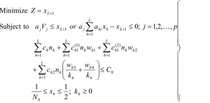
In order to obtain the optimum allocation (n*h) and sub sampling fraction (k*h) for the characteristics under study, we formulate a Bi-Objective Nonlinear programming Problem (BONLPP) as follows:
. , , 2 , 1 ; integers are and 0 ; 2 to Subject 1 1 ) ( Minimize 1 1 ) ( Minimize 0 4 3 2 2 ) 2 ( 1 1 ) 1 ( 1 1 2 2 2 1 4 ) 2 ( 2 1 2 1 3 ) 1 ( L h n k N n C k w k w n c w n c w n c n c S P w n k n y V S P w n k n y V h h h h h h h h h h h h h h h h L h h h h h L h h h h h h h L h h h h h (7)3 Several optimization techniques to solve BONLPP
3.1 Value function
Many authors studied multi objective optimization in detail such as Kish, Miettinen etc. The problem (7) expressed under value function technique as (see Diaz-Garcia and Ulloa, 2008):
.
,
,
2
,
1
;
integers
are
and
0
;
2
to
Subject
Minimize
0 4 3 2
2 ) 2 (
1 1
) 1 (
1 1
1
L
h
n
k
N
n
C
k
w
k
w
n
c
w
n
c
w
n
c
n
c
V
h
h h h
h h
h h h h h
h h h
h h L
h h h p
j j
(8)
where ϕ(.) is a scalar function that summarizes the importance of each of the variance of the p characteristics. ϕ(.) may take different forms for different problems amongst them one particular forms used here is weighted sum. Now under this approach the problem (8) can be expressed as:
.
,
,
2
,
1
;
integers
are
and
0
;
2
to
Subject
Minimize
0 4 3 2
2 ) 2 (
1 1
) 1 (
1 1
1
L
h
n
k
N
n
C
k
w
k
w
n
c
w
n
c
w
n
c
n
c
V
h
h h h
h h
h h h h h
h h h
h h L
h h h p
j j j
(9)
where
j
0
;
j
1
,
2
,
,
p
are the weights according to the relative importance of the characteristics. Without loss ofgenerality we can take
j=1
p
λ
j=1.
3.2 Fuzzy programming
Let V⋆
j be the optimal value of Vj obtained by solving the BONLPP (7). Further let
V
j~
denote the variance under compromise
allocation, where
n
h;
h
1
,
2
,
,
L
are to be worked out.Obviously,
V
~
j
V
j*or
V
~
j
V
j*
0
;
j
1
,
2
,
,
p
will give the increase in the variance due to not using the individualoptimum allocation for
j
th characteristic.To obtain a fuzzy solution, we first compute the upper and lower tolerance limits for each objective i.e.,
min
k(
*hj)
j
k
V
n
L
and)
(
max
*hj k j
k
V
n
U
, where n⋆hj denote the optimum allocation in theh
th stratum for thej
th characteristic.The differences of the maximum and minimum values of V
k are denoted by
d
k
U
k
L
k;
k
1
,
2
,
p
.
Now the fuzzy programming formulation of the BONLPP is given as:
p
j
L
h
n
k
N
n
C
k
w
k
w
n
c
w
n
c
w
n
c
n
c
i
V
d
S
P
w
n
k
n
h
h h h
h h
h h L
h
L
h
h h h
h h L
h
h h h L
h h h
j k hj h L
h
hi h h
h
,
,
2
,
1
;
.
,
,
2
,
1
;
integers
are
and
0
;
2
4
,
3
,
1
1
to
Subject
Minimize
0 4 3
1 1
2 2
) 2 (
1 1
1 ) 1 (
1 1
* 2
2
1
3.3 Goal programming
To solve the following BONLPP using goal programming, we first solve each objective subject to the system constraints separately
p
j
L
h
n
k
N
n
C
k
w
k
w
n
c
w
n
c
w
n
c
n
c
i
S
P
w
n
k
n
h
h h h
h h
h h L
h h h
L
h
h h h L
h
h h h L
h h h
hj h L
h
hi h h
h
,
,
2
,
1
;
.
,
,
2
,
1
;
integers
are
and
0
;
2
to
Subject
4
,
3
;
1
1
Minimize
0 4 3
1 2
1
2 ) 2 (
1 1
1 ) 1 (
1 1
2 2
1
(10)
Let V⋆j be the optimum value of V
j with the solution to the
th
j
NLPP as(
,
*2,
,
*).
*1 *
jL j
j
j
n
n
n
n
Further let
V
~
j the optimal value under compromise solution withn
c*
(
n
1*c,
n
2*c,
,
n
*Lc).
the vector of optimum compromise allocations for thej
thcharacteristics.Obviously,
p
j
V
V
or
V
V
~
j
j*~
j
j*
0
;
1
,
2
,
,
(11)A reasonable criterion to work out a compromise allocation may be to minimize the sum of increases in the variances,
p
j
V
j;
1
,
2
,
,
due to the use of the compromise solution. The goal is to find the compromise allocation)
,
,
,
(
1* 2* **
Lc c
c
c
n
n
n
n
such that the increase in value ofj
th variance due to the use of a compromise allocation should not exceedx
j;
j
1
,
2
,
,
p
, wherex
j
0
are the unknown goal variables.To achieve these goals x
ij must satisfy
V
~
j
V
j*
x
j;
j
1
,
2
,
,
p
or
*
~
j j
j
x
V
V
h=1
L
1n h
+
k h−1 n
h
whi P2hS2hj−xj≤V⋆j (12)
The value of
j=1
p x
j will give us total increase in the variances by not using the individual optimum allocations.
This suggests the following Goal Programming Problem (GPP) to solve:
p
j
L
h
n
k
N
n
C
k
w
k
w
n
c
w
n
c
w
n
c
n
c
i
V
x
S
P
w
n
k
n
x
h
h h h
h h
h h L
h
h h
L
h
h h h L
h
h h h L
h h h
j j hj h L
h
hi h h
h p
j j
,
,
2
,
1
;
.
,
,
2
,
1
;
integers
are
and
0
;
2
4
,
3
,
1
1
to
Subject
Minimize
0 4 3
1 2
1
2 ) 2 (
1 1
1 ) 1 (
1 1
* 2
2
1 1
(13)
The GPP (13) may be solved by using the optimization software LINGO (LINGO- User’s Guide). For more information one can visit the site: http://www.lindo.com
3.4 Chebyshev approximation
Here we consider the problem given by equation (7). For using Chebyshev Approximation we have to convert the problem into
convex programming problem so by making the transformation
h
L
x
n
h
h
;
1
,
2
,
,
1
and
1
1
2 2;
3
,
4
k
w
P
S
i
a
hj h hi h hj then the problem (8) is equivalent to minimizing the linear form (see Khan et al., 2011)p
j
k
x
N
C
k
w
k
w
n
c
w
n
c
w
n
c
n
c
x
a
V
h h
h
h h
h h L
h
h h
L
h
h h h L
h
h h h L
h
h h
L
h
h hj j
,
,
2
,
1
;
0
;
2
1
1
to
Subject
Minimize
0 4
3
1 2
1
2 ) 2 (
1 1
1 ) 1 (
1 1
1
(14)
Now the objective functions are linear and the single constraint is convex (see Kokan and Khan (1967)). So eq. (14) represents convex programming problems. The problem (14) is now equivalent to minimizing the linear form (see Ali et al., 2011)
0
;
2
1
1
,
,
2
,
1
;
0
to
Subject
Minimize
0 4 3
1 2
1
2 ) 2 (
1 1
1 ) 1 (
1 1
1 1
1 1
h h
h
h h
h h L
h h h
L
h
h h h L
h
h h h L
h h h
L L
h h hj j L
j j
L
k
x
N
C
k
w
k
w
n
c
w
n
c
w
n
c
n
c
p
j
x
x
a
a
or
x
V
a
x
Z
(15)
where a
j are the weights assigned to the variances according to their importance.
4 Illustrative example
The following example illustrates the four methods discussed in above section. The data are taken from Maqbool and Pirzada (2005) in which a population is considered which is divided into four strata. The total amount available for conducting the survey is assumed to be C=3000 units with an expected overhead cost
c
0
1000
units.
This givesC
0
C
c
0
2000
units.
The proportion of respondents are w [image:8.595.38.391.66.239.2]h1=0.4 and wh2=0.3 and the proportion of non-respondents are wh3=0.6 and wh4=0.7 for the character I and II respectively (Table 1).
Table 1. Input data for two characteristics and four strata
h N
h Ph S2h1 S2h2 ch c(1)h1 c(2)h1 ch2
1 20 0.2 3.5 3.2 0.5 8.5 8.7 25
2 30 0.3 5.5 4.8 0.7 7.4 7.6 20
3 40 0.4 6.5 6.2 0.4 7 7.2 18
4 10 0.1 5.5 5.3 0.6 9 9.2 25
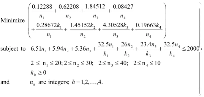
For j=1 BONLPP takes the form:
. 4 , , 2 , 1 ; integers are
and
0
10 n 2 40; n 2 ; 30 n 2 20; n 2
2000 5
. 32 4 . 23 26 5 . 32 36 . 5 94 . 5 51 . 6 to subject
1815 . 0 056 . 4 63351 . 1 294 . 0 121 . 0 704 . 2 089 . 1 196 . 0 Minimize
4 3
2 1
4 4
3 3
2 2
1 1 3
2 1
4 4
3 3
2 2
1 1
4 3
2 1
h n
k
k n k
n k
n k
n n
n n
n k n
k n
k n
k n
n n
n
h h
Above problem is solved by an optimizing software LINGO-13 and obtain the optimum solution as:
n1=12,k1=1.8660,n2=29,k2=1.7111,n3=40,k3=1.4210,n4=9,k4=1.7812
with the corresponding value of variance V1=0.4570349
For j=2 BONLPP takes the form:
. 4 , , 2 , 1 ; integers are
and
0
10 n 2 40; n 2 ; 30 n 2 20; n 2
2000 5
. 32 4 . 23 26 5 . 32 36 . 5 94 . 5 51 . 6 to subject
19663 . 0 30528 . 4 45152 . 1 28672 . 0
08427 . 0 84512 . 1 62208 . 0 12288 . 0
Minimize
4 3
2 1
4 4
3 3
2 2
1 1 3
2 1
4 4
3 3
2 2
1 1
4 3
2 1
h n
k
k n
k n
k n
k n n
n n
n k n
k
n k n
k
n n
n n
h h
Above problem is solved by an optimizing software LINGO-13 and obtain the optimum solution as:
n
1=10,k1=1.5160,n2=23,k2=1.3861,n3=40,k3=1.3279,n4=8,k4=1.4646
with the corresponding value of variance V
1=0.4058625
[image:9.595.36.380.52.216.2]To obtained the compromise allocations four methods used and according to the procedure discussed in the section 3 problems are formulated and solved by an optimization software LINGO (2013). LINGO is a user’s friendly package for constrained optimization developed by LINDO System Inc. A user’s guide-LINGO User’s Guide (2013) is also available. For more information one can visit the site http://www.lindo.com. And the results are summarized in Table 2 below:
Table 2. Compromise optimum solutions obtained by four different methods
Allocations Variances
Approaches n
1 k1 n2 k2 n3 k3 n4 k4 V1 V2 Trace=V1+V2
Value function 11 1.6850 26 1.5455 40 1.3702 8 1.5187 0.4579560 0.4067659 0.8647220 Fuzzy programming 11 1.6853 26 1.5467 40 1.3697 8 1.5179 0.4579706 0.4067673 0.8647379 Goal programming 11 1.6850 26 1.5455 40 1.3702 8 1.5187 0.4579560 0.4067659 0.8647220 Chebychev approximation 12 1.8243 29 1.7082 40 1.4189 9 1.7644 0.4570259 0.4090924 0.8661183
5 R simulation study
For comparing the efficiency of the methods discussed in section 3, a simulation study has been carried out. The R language (2011) has been used to perform the simulations and data analysis. We have generated a population of size N=1050. From this population four strata are randomly generated. The characteristics for the two populations have generated in the following way:
∼∼
Data obtained by simulation study is shown in table 1. In addition to the above, it is assumed that the relative value of the variances of the non-respondents and respondents, that is,
S
jh22S
jh2
0
.
25
for
j
1
,
2
and
h
1
,
2
,
3
,
4
. Further, let the total amountavailable for the survey be C0=1700 units for the problem (7). The proportion of respondents is wh1=0.4 and wh2=0.3 and the proportion of non-respondents is w
[image:9.595.112.483.665.729.2]h3=0.6 and wh4=0.7 for the character I and II respectively.
Table 3. Input data for two characteristics and four strata
h N
h Ph S2h1 S2h2 ch c(1)h1 c(2)h1 ch2
1 306 0.291429 5800.17 2385.23 0.5 8.5 8.7 25
2 205 0.195238 555.248 160.637 0.7 7.4 7.6 20
3 353 0.33619 1592.11 684.948 0.4 7 7.2 18
4 186 0.177143 5464.03 1749.39 0.6 9 9.2 25
For j=1 BONLPP takes the form:
. 4 , , 2 , 1 ; integers are
and
0
186 n 2 353; n
2 ; 205 n 2 306; n 2
1700 5
. 32 4 . 23 26 5 . 32 36 . 5 94 . 5 51 . 6 to subject
71886 . 25 99192 . 26 174731 . 3 89185 . 73
14591 . 17 99461 . 17 116488 . 2 26123 . 49
Minimize
4 3
2 1
4 4
3 3
2 2
1 1 3
2 1
4 4
3 3
2 2
1 1
4 3
2 1
h n
k
k n
k n
k n
k n n
n n
n k n
k
n k n
k
n n
n n
h h
Above problem is solved by an optimizing software LINGO-13 and obtain the optimum solution as:
731488
.
1
,
17
,
687236
.
1
,
20
,
815039
.
1
,
7
,
802684
.
1
,
30
1 2 2 3 3 4 41
k
n
k
n
k
n
k
n
with the corresponding value of variance V1=14.01262.
For j=2 BONLPP takes the form:
. 4 , , 2 , 1 ; integers are
and
0
186 n 2 353; n
2 ; 205 n 2 306; n 2
1700 5
. 32 4 . 23 26 5 . 32 36 . 5 94 . 5 51 . 6 to subject
606634 . 9 54773 . 13 071551 . 1 4513 . 35
117129 . 4 806169 . 5 459236 . 0 19342 . 15
Minimize
4 3
2 1
4 4
3 3
2 2
1 1 3
2 1
4 4
3 3
2 2
1 1
4 3
2 1
h n
k
k n
k n
k n
k n n
n n
n k n
k
n k n
k
n n
n n
h h
(20)
Above problem is solved by an optimizing software LINGO-13 and obtain the optimum solution as:
365949
.
1
,
13
,
351395
.
1
,
18
,
406972
.
1
,
5
,
476810
.
1
,
27
1 2 2 3 3 4 41
k
n
k
n
k
n
k
n
with the corresponding value of variance V
1=5.560957.
[image:10.595.36.383.52.216.2]To obtained the compromise allocations four methods used and according to the procedure discussed in the section 3 problems are formulated and solved by an optimization software LINGO (2013). LINGO is a user’s friendly package for constrained optimization developed by LINDO System Inc. A user’s guide-LINGO User’s Guide (2013) is also available. For more information one can visit the site http://www.lindo.com. And the results are summarized in table 4 below:
Table 4. Compromise optimum solutions obtained by four different methods
Allocations Variances
Approaches n
1 k1 n2 k2 n3 k3 n4 k4 V1 V2 Trace=V
1+V2
Value function 29 1.695526 6 1.592187 20 1.629516 16 1.645804 14.03011 5.597118 19.627228
Fuzzy programming 29 1.657579 6 1.648854 19 1.502105 15 1.571902 14.0666 5.579078 19.645678 Goal programming 29 1.695526 6 1.592187 20 1.629516 16 1.645804 14.03011 5.597118 19.627228 Chebychev approximation 30 1.824339 7 1.708236 20 1.706003 17 1.764377 14.09261 5.674545 19.767155
6 Conclusion and Future work
In this article a Bi-objective nonlinear programming problem is formulated from bivariate stratified problem under partial responses. The problem of finding optimal allocations has been solved using four different methods viz. Value function, Fuzzy programming, Goal programming and Chebyshev approximation. Optimum compromise solution (Table 2) obtained by real life data shows that the value function and goal programming methods provides the most efficient solution. To check the efficiency of the results a simulation study has been carried out which also conclude that the value function and gaol programming methods give the most efficient solution. The comparison of the results has been graphically shown in the figure given below. In future one can check the efficiency of the methods for more than one population and can also try to formulate the problem under partial responses as a multi objective programming problem i.e p≥2.
Acknowledgement
The first author is thankful to University Grant Commission, New Delhi, India for providing BSR-SRF and the second author is thankful to University Grant Commission to provide financial assistance under the UGC Start-up grant No.F.30-90/2015 (BSR), Delhi India to carry out this research work.
REFERENCES
Ali, I., Raghav, Y.S., and Bari, A. 2011. compromise allocation in multivariate stratified surveys with stochastic quadratic cost function, Journal of Statistical computation and Simulation, DOI:10.1080/00949655.2011.643890.
Díaz-García, J.A., Ulloa, C.L. 2008. Multi-objective optimisation for optimum allocation in multivariate stratified sampling.
Survey Methodology, 34(2), 215–222.
El-Badry, M.A. 1956. A sampling procedure for mailed questionnaire. Jour. Amer. Stat. Assoc, 51, 209-277.
Fabian C. Okafor and Hyonshil Lee 2000. Double sampling for ratio and regression estimation with sub sampling the non respondents. Survey Methodology, Vol. 26, (2), pp 183-188.
Gupta, N., Ali, I., Bari, A. 2013. An Optimal Chance Constraint Multivariate Stratified Sampling Design Using Auxiliary Information, J Math Model Algor, DOI 10.1007/s10852-013-9237-5
Gupta, N., Shafiullah, Iftekhar, S. and Bari, A. 2012. Fuzzy Goal Programming Approach to solve Non-Linear Bi-Level Programming Problem in stratified double sampling design in presence of non-response, International Journal of Scientific & Engineering Research, Volume 3, Issue 10, October - 2012 ISSN 2229-5518.
Hansen,M.H., Hurwitz,W.N. 1946. The problem of non response in sample surveys, J. Amer. Statist. Assoc., 41, 517-529
Khan, M. G.M., Khan, E.A., Ahsan, M.J. 2008. Optimum allocation in multivariate stratified sampling in presence of non-response, J. Indian Soc. Agricultural Statist., 62(1), 42-48
Khan, M., Ali, I., Raghav, Y. S. and Bari A. (2012). Allocation in Multivariate Stratified Surveys with Non-Linear Random Cost Function, American Journal of Operations Research, 2 (1), 100-105
Khare,B.B. 1987. Allocation in stratified sampling in presence of non response, Metron., 45(1-2), 213-221
Kokan A.R., Khan S.U. 1967. Optimum allocation in multivariate surveys: an analytical solution. J R Stat Soc B., 29(1), 115–125. Kozak, M. 2006. On sample allocation in multivariate surveys, Comm. Statist. Simulation Comput., 35(4), 901-910
LINGO-User’s Guide 2013. "LINGO-User’s Guide". Published by LINDO SYSTEM INC., 1415, North Dayton Street, Chicago, Illinois, 60622 (USA)
Maqbool, S. and Pirzada, S. 2005. Allocation to response and non-response groups in two character stratified sampling, Nihonkai Math. J., Vol.16, 135-143 USA.
Miettinen, K.M. 1999. Non linear multiobjective optimization, Kluwer Academic Publishers, Boston
Najmussehar, Bari, A. 2006. Double sampling for stratification with sub-sampling the non-respondents: a dynamic programming approach, Aligarh J. Statist., 22, 27-41 (2002)
R Development Core Team. 2004. R: A language and environment for statistical computing, Vienna, Austria: R foundation for statistical computing. http://www.R-project.org.
Raghav, Y.S., Ali, I., Bari, A. 2010. Optimum Sample Sizes in Case of Stratified Sampling for Non-Respondents : An Integer Solution, International Journal of Operations Research and Optimization, Volume 1, No. 1, pp. 149-160
Steuer, R.E. 1986. Multiple criteria optimization: Theory, computation and applications, New York, John Wiley & Sons, Inc Varshney, R., Najmussehar, Ahsan, M. J. 2011. An optimum multivariate stratified double sampling design in non-response,
Springer, Optimization letters. Verlag