Should we pay for ecosystem service outputs, inputs or both?

Should We Pay for Ecosystem Service Outputs, Inputs or Both?

Abstract

Payments for ecosystem service outputs have recently become a popular policy prescription

for a range of agri-environmental schemes. The focus of this paper is on the choice of

instruments in contracts to incentivise the provision of ecosystem service outputs from farms.

The farmer is better informed than the regulator in terms of hidden information about costs

and hidden-actions relating to effort. Results show that with perfect information, the regulator

can contract equivalently on inputs or outputs. With hidden information, input-based

contracts are more cost effective at reducing the informational rent related to adverse

selection than output-based contracts. Mixed contracts are also cost-effective, especially

where one input is not observable. Such contracts allow the regulator to target variables that

are “costly-to-fake” as opposed to those prone to moral hazard such as effort. Further results

are given for fixed price contracts and input-based contracts with moral hazard. The model

is extended to include a discussion of repeated contracting and the scope that exists for the

regulator to benefit from information revealed by the initial choice of contract. Results are

illustrated with a case study of contracting with farmers to protect high biodiversity native

1

Introduction

The provision of ecosystem services and biodiversity conservation may be seen in some environments as a process of accumulating and maintaining the natural capital assets that support ecosystem service (ES) output. It is an investment decision that requires diverting land, labour and man-made capital to appreciate an ecosystem asset, which in turn provides an ES output. For instance, in the case study discussed later in this paper, the ecosystem asset is an area of endangered Australian native vegetation that hosts unique biodiversity but also provides ecosystem services including regulating saline ground water and reducing soil erosion. Without sufficient land and effort allocated to its protection, the state of native vegetation depreciates. If the vegetation remnant is recruited into a conservation management scheme then both the area and its condition can appreciate, increasing the shadow value of this asset. The definition of an ES used here is consistent with Bateman et al (2011), Barbier (2009) and Mäler et al. (2009). To quote Bateman et al. (2011, p180) “the level of ecosystem service ‘harvested’ within any given period can be thought of as a ‘flow’ extracted from an

underlying ‘stock’ of ecosystem asset….”.

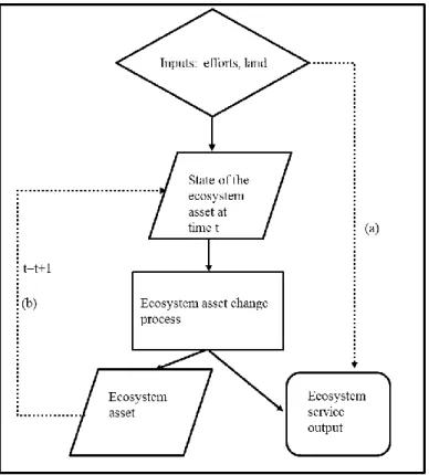
The process described is characterised by the flowchart in Figure 1. A land area has an ecosystem asset of a given state as measured by a metric. This is combined with input factors land and conservation effort, and through an ecosystem asset change process provides an ES output. The process is dynamic, since the ecosystem asset changes through time. Contracting with owners and/or managers of the asset can be used at a number of stages in this process: such contracts can specify the inputs employed by the land manager, the state of the

Note: the diagram indicates input decisions with a diamond; a state variable (ecosystem asset) with a rhomboid, a process (the ecosystem change process) with a rectangle and a flow variable ecosystem services as round–cornered rectangle.

Figure 1 Conceptual model linking ecosystem outputs, inputs and assets

However, output-based payments have advantages (Gibbons et al., 2011). For instance, if essential inputs are hidden (or expensive for the regulator to observe), then paying for outputs may be more efficient. Moreover, farmers may hold private information on the best methods for investing in the ecosystem asset and producing the ES: these cannot be easily specified in an actions-based contract. Output-based payments encourage land managers to make use of this information to produce ES outputs.

One economic approach to the design of voluntary agri-environmental schemes is based around mechanism design, structuring contracts to induce a dominant-strategy Bayesian equilibrium in games of incomplete information (Laffont and Tirole, 1993). This mechanism is applied to define a menu of contracts that is designed to separate “types” of supplier by voluntary self-selection, as a means of reducing information rents. We follow this approach in the model set out in section 3.

The rest of the paper is organised as follows. Section 2 provides a brief literature review. Section 3 presents the models. The first subsection gives the derivation of the compliance cost. The next sets out the first-best perfect information solution. The hidden information contracting problem is analysed using input, output and mixed contracts. An alternative price-based contract is then analysed which is characterised as one approach to overcoming moral hazard. Moral hazard is also addressed directly as a problem of allocating monitoring resources. The last subsection considers the input-based contract over two periods with the possibility of re-contracting. Section 4 gives an empirical example. Section 5 concludes and identifies areas for further research.

2

Literature Review

another must “ be due to inadequate information or uncertainty.” This paper, along with the literature on procurement and contracting (Laffont and Tirole, 1993; Laffont and Martimort, 2002) has led to a number of papers applying mechanism design to agri-environmental polices (Wu and Babcock, 1996 and Moxey et al., 1999; Ferraro, 2008; Hanley et al., 2012 and Miteva et al., (2012).

Recent papers that have specifically looked at the optimal selection of alternative policy mechanisms include Melkonyan and Taylor (2013). They show in relation to policy for US ranchland that, given informational asymmetries between ranchers and regulators, outcome- based payments are a first-best policy when regulators can perfectly monitor the ecological condition of the ranch. Where monitoring is imperfect, input regulation and cost-sharing or taxation may dominate performance regulation. Anthon et al. (2010) consider the optimal design of PES-type contracts to private landowners under asymmetric information. They find foresters who are likely to achieve a higher level of conservation should be offered output-based contracts. Derissen and Quaas (2013) extend a model by Zabel and Roe (2009) to develop a mixed output-based and input-based contracting approach to a problem where the farmer is better informed about environmental performance than the regulator. Their model addresses asymmetric information relating to the marginal productivity of the “ecosystem production function”. Under such conditions, they show that a mixed contract on inputs and output is preferred.

Dynamic contracting, commitment and renegotiation is critical to the long term protection of ecosystem assets, as positive change is often gradual and degradation rapid and irreversible. However, there has been a limited application of principal-agent models from general economics (Laffont and Tirole, 1988, 1990) to long term contracting for ecosystem services. The key issues in this literature (Rey and Salanie, 1990 and 1996) are the role of commitment by the regulator to set up separating contracts and the use of spot contracts as alternatives to long term contracts. The contribution of this paper is to take a general procurement model due to Laffont and Tirole (1993) and modify it in a way that relates more closely to the realities of ES output contracts. In particular, we consider a situation in which there are two inputs and a single ES output related by an ecosystem production function. Further, the farmer is

generalisations allow us to explore the role of differentiated transactions costs related to the monitoring of contract variables. These issues are reviewed by reference initially to a two-type static model, and then to a two-period, two-two-type dynamic model.

3

The Model

This section sets up a general agri-environmental contract for providing ecosystem services, and then explores aspects of the model to assess when payment for ecosystem output or payment for ecosystem inputs is optimal. Assume that there are just two representative farmer types that are able to provide an ES, the supply of which depends on how land is managed in a region. These farmer types differ according to their agricultural productivity, information on which may be hidden from the regulator. Thus, there is hidden variation in the opportunity costs of providing ecosystem inputs since the ES output requires the sacrifice of inputs used to produce profitable crops. Farmers combine land and effort to invest in an ecosystem asset that in turn provides an ES output. The benefits can be measured as an

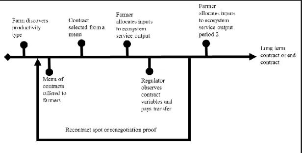
ecosystem metric, where the changes in the metric can then be valued. The contract timing for a general problem, including repeated contracting, is given in Figure 2.

Aspects of the standard model that are explored here include the number of inputs, farm types and information. The standard principal-agent model for procurement, for instance Laffont and Martimort (2002, Chapter 3), typically has a single input variable “effort”. This

Figure 2 Contract timings

3.1 Compliance costs

The costs of engaging in providing an ecosystem service are internal to the farm business in the sense that the farmer allocates resources such as land and effort to maintain the ecosystem asset. To represent this, we define a restricted profit function (Lau, 1976) with fixed land and effort as 0   ( _ix, _ie,p w xa, a, _tia, e )_tia , where 0 is the baseline agricultural profit. Here, θ , is the farmer’s type (defined on either land productivity, x

i

 , or effort productivity , e i  , or both), pa are crop output prices, a

w is a vector of price for variable inputs such as fertilizer, and a

i

x and ea

i are respectively land and effort allocated to agriculture. The productivity parameters and market prices are assumed fixed in all time periods of the model. Each farmer can identify the optimal profit from farm production and this allows her to make a profit-maximising choice over other variable inputs such as pesticides and fertilizers. The restricted profit function provides a way of describing a compliance cost function where resources x_i

(land) and e_i(effort) are re-allocated from crop production to conservation:

0

( ix, ie, ti, e )ti ( ix, ie a, a, tia ti, etia ti)

Compliance cost is thus baseline profit minus profit with land and effort allocated to producing ES output. To make the analysis tractable we assume that the compliance cost function (1) is approximated by the separable quasi convex function:

( _ix, _ie, _ti, e )_{ti x}( _ix, _ti) _e( _ie, _ti)

c  x c  x c  e . (2)

Cost functions are strictly increasing in the type parameters.

3.2 General contracting problem

This section sets up the general contracting problem as a basis for considering the potential for different contract designs. The risk neutral regulator maximises a social welfare function:

1. , , ,

ti

( , , y ) ( , ) ( , )

(1+ )c ( , ) ( +p y )

ti ti ti ti

e x

ti ti t i e i ti x i ti t i

x e f p

t i m ti ti ti ti

vg x e c e c x

Maximum

e x f

 

 

 



   

 

 

 

 

 

 

(3)

The term _t is the discount factor for period t and _i is the probability of a firm being of type

i.1_{The term v indicates the economic value per unit of increase in the ecosystem asset. The} regulator maximizes the expected present value of the ES output given by the difference equation that describes the ecosystem ‘production function’or asset change process

1,

y_ti g x e( _ti, _ti, y_{t i}) for farm type i,. The ES output depends directly on the current level of the ecosystem asset. The term c ( ,m e xti ti) is the cost of compliance monitoring. Policies can include direct contracts for land, effort or output. The farmer receives payments either as lump-sum transfers f_tiand/or as a per-unit-of-output payment p y_{ti ti}. In the social welfare function, transfers are weighted by the shadow price of public funds 01. This term accounts for the cost of raising tax revenue due to the deadweight loss of taxation (Campbell and Bond, 1997).

Assuming compliance so that the problem for the farmer is deterministic, the farmer’s objective function is





, ( , ) ( , )

ti ti

t e x

ii ti ti ti e i ti x i ti

e x t

J Maximize



The profit to the farmer when they truthfully reveal their type is indicated by the subscripts ii.

The participation constraint is:

ii i

J J (5)

where J_i is the farm’s reservation profit. The incentive compatibility constraint is:

,

ii ij

J J i j. (6)

The first subscript is the farm’s type whilst the second subscript is the farm’s declared type when selecting from a menu of contracts. The regulator acts as a Stackelberg leader (Baron, 1985) in optimizing (3) constrained by (4), (5) and (6). In the analysis we start with a simple model and develop a set of results for aspects of the general model.

3.3 Static first-best input and output-based contracts

Assumptions A1. The regulator maximizes the social-welfare function, and is risk neutral.

They can also estimate, v,_i, and the ecosystem production function y_ti g x e( _ti, _ti, y )₀ . The

regulator observes the farm types. Farm types are either high land productivityh or low land

productivity l types, with x x

h l

  . Each farm has an identical ecosystem asset at the start of

the period and thus this term can be dropped from the production function along with the time

subscript y_i g x e( , )_{i i} . The effort productivity e is the same for both farm types, and

farmers are risk neutral.





, , ( , ) ( , ) ( , ) - ,

i i i

e x

i i e i x i i i

x e f

Maximum vg x e c  e c  x f il h (7)

subject to the individual rationality or participation constraint:

( ( e, ) ( x, )) 0 ,

i e i x i i

f  c  e c  x  il h (8)

The optimal internal solution is:

' '

(1 ) ( , ); (1 ) ( , ) ,

i i

e x

e e i x x i i

vg   c  e vg   c  x il h (9)

The shadow cost of public funds increases the marginal cost of input allocations. The first-best policy is least cost as (9) implies the condition for cost minimization:

' ' ( , ) , ( , ) i i e

e _{e i}

x

x x i i

g c e

i l h

g c x

 

  (10)

If instead the regulator contracts only on ES output y_i, the firm, as the residual claimant, produces the contracted output at a minimum cost. Define a cost function as:

0

( , ) [ ( e, ) ( x, ) : ( )] ,

y i i e i x i i i i

z

c  y Minimum c  e c  x z Z y i l h



    ₍₁₁₎

where

z

regulator is:





, ( , ) - ,

i i

i y i i i

y f

Maximum vy c  y f il h ₍₁₂₎

and the participation constraints:

( , ) 0 ,

i y i i

The shadow cost of public funds, , increases the marginal cost of the ES output. The input-based and outcome-input-based contracts are identical as, by definition, the cost function (11) implies cost minimization

) , ( ) 1

( c'_{y i} y_i

v   . (14)

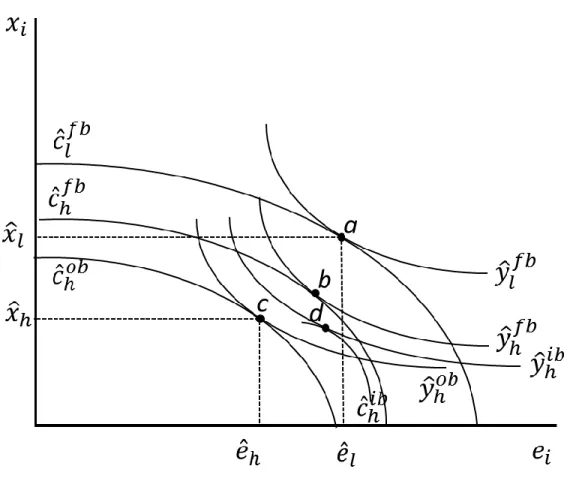
The input-based contract is also cost minimizing as (10) implies a cost minimizing solution. The first-best contracts are illustrated in Figure 3. The regulator would offer the low-cost farm type (l-type) the contract at a as either an input-based or an outcome-based contract, and the high-cost farm type (h-type) the contract at b. For an input contract the regulator, as the residual claimant, sets the contracted levels of effort and land to minimize the transfer payment related to a level of output and thus maximize the social welfare function. For the output contract. farmers as residual claimants select the cost minimizing levels of input to maximize their profit.

Result 1. The first best input and output contract are equivalent and lead to the same social

welfare, ES output and input mix.

3.4 Adverse selection with an input-based contract

Assumptions A2. Assumptions A1 hold except that the regulator does not observe the land

productivity parameter directly, but has a subjective estimate of the probabilityi of each

farm type.Effort productivity is the same for both types.

The objective function is modified to give the expected social welfare function:





, , ( , ) ( , ) ( , )- ,

i i i

e x

i i i e i x i i i

x e f i

Maximum



where _i is the probability of a farm being of type i. Thus the objective function (15) is maximised subject to the participation constraints (8) and incentive compatibility (IC-i)

( e, ) ( x, ) ( e, ) ( x, ) , , ;

i e i x i i j e j x i j

f c  e c  x  f c  e c  x i jl h i j (16)

The assumptions of strictly convex cost functions and the single-crossing property of the incentive compatibility constraints ensure that the individual rationality for the h-type(IR-h)

and incentive compatibility constraint for the low cost (IC-l) type are the only binding

constraints (see Appendix 1). The l-type earns a rent and the h-type has a zero rent. The rent is defined at the optimal solution ˆ ˆ{ , }e x_{i i} by rˆ_i  fˆ_i c_e(e, )eˆ_i c_x(_ix, )xˆ_i . With these

additional restrictions, the objective function (15) can be rewritten as:





, , ( , ) (1 )( ( , ) ( , )- ,

i i i

e x

i i i e i x i i i

x e f i

Maximum



By assumption rent for the h-type farmer is zero and from the binding (IC-l):

( e, ) ( x, ) ( e, ) ( x, ) = ( x, ) ( x, )

l e h x h h e h x l h x h h x l h

r c  e c  x c  e c  x c  x c  x .

On this basis the optimal internal solution gives two first-order conditions, the first for the l-type:

' '

(1 ) ( , ); (1 ) ( , )

l l

e x

e e l x x l l

vg   c  e vg   c  x (17)

(thus the l-type is offered the first-best solution) and the second for the h-type:

' ' l ' '

h

(1 ) ( , ); (1 ) ( , ) ( ( , ) ( , ))

h h

e x x x

e e h x x h h x h h x l h

vg  c  e vg  c  x  c  x c  x 

      . ₍₁₈₎

The second term on the right-hand side of the first-order condition for land is positive by assumption and measures the marginal information rents associated with increasing the input requirements in the contract for the h-type. This term also means that the input requirement is no longer resource cost minimizing for the given ES output:

' '

'

' l ' '

h ( , ) ( , ) < ( , ) ( , ) ( ( , ) ( , )) (1 ) h h e e

e e h e h

x

x x x

x x h h

x h h x h h x l h

g _{c e c e}

g _{c x c x c x} c x

This indicates that the land to effort ratio for the h-type is reduced due to the additional marginal information rent.

Result 2 The l-type is offered the first best input level, but is paid an information rent in excess

of the compliance cost. The h-type is offered a contract with a lower level of land and effort,

and their information rent is zero.

3.5 Adverse selection with an output-based contract

Assumption A3. As for A2 except the regulator contracts on the ES output.

From an output contract perspective, the problem is re-stated as follows:





, ( , )- ,

i i

i i y i i i

y f i

Maximum



Subject to the individual rationality constraint:

( , ) 0 ,

i y i i

f c  y  il h (21)

and incentive compatibility constraints:

( , ) ( , ) , , ;

i y i i j y i j

f c  y  f c  y i jl h i j. (22)

The first order condition for the l- type is:

) , ( ) 1

( c'_{y l} y_l

v   . (23)

For the h- type the output is reduced compared to the first-best:

' l ' '

h

(1 ) _y( _h, _h) ( _y( _h, _h) _y( ,_{l h}))

v  c  y  c  y c  y 

    . ₍₂₄₎

first-best, but, as the farm is the residual claimant for any cost reductions, a profit maximizing farmer produces the contracted ES output at a minimum cost (one of the claimed advantages of outcome-based contracts noted in the introduction). This contrasts with (18) where the inputs are fixed by the regulator and the h- type can be induced to select an input combination which has a higher proportion of effort than the cost minimizing solution.

Note: 1. yˆ_hib, indicates the isoquant for the adverse selection problem input-based (ib) 2. yˆ_hob indicates outcome-based (ob). 3. The isocost curve cˆib_h is for adverse selection input-based and includes the informational rent. 4. The isocost cˆ_hob is for the outcome-based contract.

Figure 3 Input-based and output-based contracts

constrains the solution to be at the cost minimizing combination of inputs, and the total cost (resource cost plus information rent) of the ES output is not minimized due to the information rent.

Result 3. With adverse selection, an input contract is weakly preferred by the regulator to an output contract, as it solves the mechanism design problem at least cost. This result is equivalent to the result derived by Khalil and Lawaree (1995) for a single input model.

Intuitively this result holds trivially because with an input-based solution the regulator can

always select the least cost inputs. Restricting the solution to an output-based contract adds

an additional constraint and so increases the cost of mechanism design.

3.6 Adverse selection with a mixed contract

Assumption A4. As in A2, except that the regulator contracts on land and the ES output, but

not effort directly. Effort is non-verifiable.

Instead of contracting directly on effort, a second-best optimal effort is induced by contracting on land and output. Effort is selected by the agent to solve:

ˆ ˆ ˆ ˆ ˆ

( , ) argmin[ ( e, ); ( , ), ]

i i i e i i i i i i

e x y  c  e y g x e x x . (25)

where ˆx_iand ˆy_iare the contracted levels. Substituting the effort function e x y_i( ,_{i i}) into the regulator’s objective function:2





, , ( , ( , )) ( , ( , )) ( , )- ,

i i i

e x

i i i i i e i i i x i i

x y f i

Maximum



The objective function (26) is maximised subject to participation constraints:

2 _{The existence of this function is easily shown for the production function} ˆ ˆb1 b2

i i i

y x e , rearranging effort is given by ₍ˆ ˆ_{, ) (}ˆ _/ ˆb1₎1/b2

i i i i i

( e, ( , )) ( x, ) 0 ,

i e i i i x i i

f c  e x y c  x  il h. (27)

and incentive compatibility constraints:

( e, ( , )) ( x, ) ( e, ( , )) ( x, ) , , ;

i e i i i x i i j e i i i x i i

f c  e x y c  x  f c  e x y c  x i jl h i j₍₂₈

)

The results given in Appendix 2 show that this result is equivalent to the optimal input-based solution. The approach of contracting on variables that are more readily observable can be generalised to other contract settings, but depends on the existence of the function e x yi(ˆ ˆi, i),

that relates observable variables to unobservable ones. An equivalent version of this result can be derived for the case where the land type is the same, but the effort type is differentiated between producers. This follows as the result does not rely on the observability of effort, only the fact that the verifiable land and output uniquely determine effort.

Result 4. A mixed contracton output and land is equivalent to the optimal input-based

solution to the adverse selection problem.

A short discussion about possible generalisations of this result is warranted. For a contract to be viable, the regulator must be able to contract on sufficient variables, with active monitoring if required, to ensure production of the ecosystem service. Thus, an input contract is not viable if one essential input is not observable or contractible. In contrast, if an ES output is observable and the contract is based on outputs, this does not depend on input observability as the agent as residual claimant has an incentive to produce the contracted output at least cost. Settings where the extra information rent for a third-best output-based contract is relatively low and the transaction cost of observing inputs is higher than for output, favours output-based contracts.

production function, it may be possible to construct an aggregate type that accounts for differences in both land and effort productivity. For instance, if the opportunity cost functions are linear and the ecosystem production function is Cobb-Douglas:

1 2 [ _ix _{i i}e _i; subject to: _{i i}b _ib ]

Minimize x  e y x e

the aggregate type measure is given by:

 

 

3.7 Moral hazard

Assumption A5. As in A2, except that effort is costly to monitor and the regulator can

penalize the agent for the level of non-compliance (shirking).

If a contracted input is unobservable without the regulator engaging in costly monitoring then this creates a moral hazard problem, as the farm may shirk on the contracted level of input use. Within the model developed here, two approaches emerge for dealing with moral hazard; either direct monitoring with penalties, or mixed contracts where the contract specifies

“costly-to-fake” variables such as ES output and land use. These are sufficient to ensure an optimal level of the unobservable variable. If, for instance, ES output is costly to measure, then the regulator may have to monitor effort directly and use an input-based contract. The effectiveness of monitoring depends on the capacity of the regulator to charge a fine for applying less effort than contracted (White, 2002). Assume that monitoring frequency lies in a range 0 m 1and has a linear cost cmof monitoring. The fine per unit of effort

undersupplied (relative to the contracted level of effort) is . The regulator’s objective function is:





, , ( , ) ( , ) ( , )- -(1+ ) ,

i i i

e x

i i e i x i i i m

x e f

Maximum vg x e c  e c  x f  mc il h. (29)

ˆ 0 ( )

ˆ ˆ

( e) .

e e

e

e e e

        _{ }  (30)

Ozanne and White (2007) show that a solution is feasible if a moral hazard incentive constraint is satisfied:

'

( ) m

e i

c e   (31)

The objective function (29) is maximised subject above constraint, the IR-h (8) and the IC-l

(16) constraints. The first order condition for effort is:

' ''

(1 )( ( , ) ( , )) , .

i

e m e

e e i e i

c

vg  c  e c  e i l h



    (32)

Notably, the monitoring term is strictly positive and increases the marginal cost of effort. Relative to the solution, given by (19), monitoring reduces the land to effort ratio:

' ''

' '

' l ' '

h ( , ) ( , ) ( , ) < . ( , ) ( , ) ( ( , ) ( , )) (1 ) h h

e m e

e

e h e h

e _{e h}

x

x x x

x x h h

x h h x h h x l h

c

c e c e

g c e

g _{c x c x c x} c x

  _              (33)

Result 5. The regulator monitoring contract is less cost-effective than either the input-based

or mixed contract, as the second term on the right-hand side of (32) reduces the optimal effort to land ratio.

3.8 Price-based contracts

Assumption A6. The regulator observes farm types and offers each a price contract based on

the ES output. The regulator does not contract directly on inputs or output. The output

depends upon the farmer’s supply response for ES output. The regulator is able to observe

A perfect information price contract is where the regulator acts as a price discriminating monopsony and has perfect information about types. The regulator’s objective function is:





i

i i y i i i

p i

Maximum



subject to:

( ) argmax[ ( , )] ,

i i i i y i i

y p  p y c  y il h. (35)

The first-order conditions are:

' i 1 '

'

y ( )

(1 ) ( , ) (1 (1 ( ) )) ( , )

y ( )

i

y i i i y i i

i i p

v c y p c y

p 

     

      ₍₃₆₎

where (pi)is the price elasticity of conservation output with respect to price A first-best

price contract is sub-optimal to a first-best output-based contract and entails less conservation output for a given budget due to the cost of paying both types a rent . For any arbitrary ES output, a regulator would prefer to pay the cost rather than an output price. Comparing p_iy_i and cy( ,i yi), to incentivise some level of output y and i

'

= ( , ) i y i i

p c  y , for a strictly convex cost function and positive levels of output, p y_{i i} c_y( ,_i y_i)implies that marginal cost is greater than the average cost that is c'_y( ,_i y_i)c_y( ,_i y_i) /y_i. Thus the transfer payment for a given output is higher under a price-based contract than under an output scheme.

Assumption A7. The same as A6 except that the regulator does not observe type and offers all

types a single price.

If only a single price is offered to both producers, then the optimal solution is:

' ' ' '

(1 ){ l y( ,l l) h y( ,h h)} ( l l h h)/( y (l l l) hy (h h)).

v  c  y  c  y  y  y  p  p (37)

Result 6. In a first-best price based contract compared to a first-best input contract the ES

output is reduced due to the public cost of rent from supplying the ecosystem service.

Result 7. If the regulator addresses hidden information by offering a single price, the optimal

solution is determined by the expected values of first-order condition (37). The averaging effect means that the l-type has output less than or equal to and the h-type an output greater than or

equal to the first-best price contract.

3.9 Two-period and repeated contracts

Assumptions A8. The assumptions are the same as A2 for the input-based contact with

adverse selection. Specific assumptions for the two-period contract include inputs in the first

period appreciate the ecosystem asset in both that period and in the second. Producer types

are stable over the two periods. The initial condition of the ecosystem asset is the same for

both types at y0. A total transfer payment variable is paid for each type 1 2

r

i i i

f  f  f which

gives the present-value of payments over the two periods. The farmers and regulator have an

identical discount factor,  . The duration of periods may be unequal.

the model is due to Laffont and Tirole (1993, Chapter 2). The difference with their model is that farmers are investing in an ecosystem asset so that the problem changes through time. Commitment by the regulator is critical for investment in ecosystem assets as it can prevent incentives that could arise for farmers to first invest in the ecosystem asset and then

subsequently dis-invest. Contracting with commitment is viewed as a process of managing the ecosystem asset in a transition towards equilibrium where the agent’s type is known and they are paid in a long term contract to maintain the equilibrium. At this stage the regulator may offer the agent a covenant to permanently protect the asset. In this section we explore this transition towards equilibrium.

The regulator’s objective function over two periods is:

1 1 0 1 1

,e ,

2 2 1 2 2

( ( , e , y ) ( , ) ( , )

, ; t 1, 2.

( ( , e , y ) ( , ) ( ,

))-r ti ti i

e x

i i e i x i i

i _{e x r}

x f _i

i i i e i x i i i

v g x c e c x

Maximum i l h

vg x c e c x f

             _{  }        



This is optimised subject to the participation constraints:

1 1 2 2

( , ) ( , ) ( ( , ) ( , )) 0 ,

r e x e x

i e i x i i e i x i i

f c  e c  x   c  e c  x  il h (39)

and the incentive compatibility constraints:

1 1 2 2

1 1 2 2

( , ) ( , ) ( ( , ) ( , ))

( , ) ( , ) ( ( , ) ( , )) , , ;

r e x e x

i e i x i i e i x i i

r e x e x

j e j x j j e j x i j

f c e c x c e c x

f c e c x c e c x i j l h i j

    

    

     

       . (40)

The first-order conditions are derived on the basis that the individual rationality constraint for the h-type and the incentive compatible constraint for the l-type are binding. The effort conditions are the same for both types:

1 1 1

' 1

( ) (1 ) ( , )

i i i

e

e y e e i

v g g g   c  e ;

2

' 2

(1 ) ( , ) , i

e

e e i

Effort in the first period increases the ecosystem asset in the first and second period. In common with the static solution (17) and (18) the optimal land allocation for the low cost type is the first-best:

1 1 1

' 1

( ) (1 ) ( , )

l l l

x

x y x x l l

v g g g   c  x ;

2

' 2

(1 ) ( , )

l

x

x x l l

vg   c  x . (42)

The h-type marginal condition includes two informational rents one for each period:

1 1 1

' ' '

1 1 1

( ) (1 ) ( , ) ( ( , ) ( , ))

h h h

x l x x

x y x x h h x h h x l l

h

v g g g  c  x  c  x c  x 

     ₍₄₃₎

2

' ' '

2 2 2

(1 ) ( , ) ( ( , ) ( , ))

h

x l x x

x x h h x h h x l l

h

vg  c  x  c  x c  x 

    . ₍₄₄₎

Embedded in this problem is an issue of the length of contracts and the duration of each stage. The regulator may make the first period short so that the performance of firms can be

observed, possibly by active output monitoring (White, 2005), and the second period longer as the regulator offers the farms revised Pareto improving contracts.

Result 8. With two period and repeated contractsthe regulator may commit to allow the

l-type producer to earn and information rent in both periods. Any renegotiation cannot make

the agents worse off. However, a renegotiation that increases inputs from the h-type in the

second period and maintains or increases the rent to the l-type may improve

cost-effectiveness.

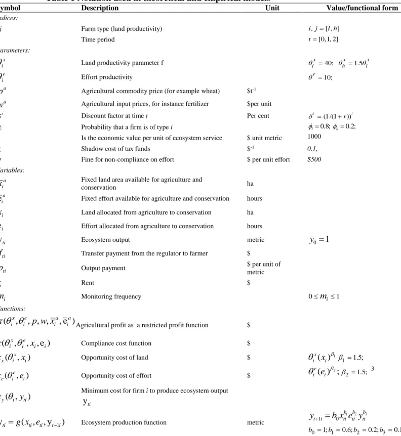
Table 1 about here

4

A case study

The south-west corner of Western Australia is designated by Conservation International as a Biodiversity Hotspot (Myers et al., 2000). This designation indicates a region of high

has only around 12% of its indigenous, native vegetation remaining. The role of input and output based agri-environmental schemes in protecting this ecosystem and the characteristics of the study region is described in detail by White and Sadler (2012).

The remaining biodiversity in the region is found in remnant woodland, shrub and mallee heath, collectively termed “bush remnants”. The threats to biodiversity include land clearing for cereal and sheep production (although further clearing is banned), the encroachment of agricultural weeds, and sheep grazing. Management practices include excluding sheep through fencing, weeding and replanting. The regulator (the Western Australian Department of Parks and Wildlife) can identify the area of land that is fenced and included in a

conservation scheme at low cost. However, other conservation efforts by the farmer are almost impossible to observe and record in a way that is legally enforceable. Similarly, the management of sheep grazing is difficult to observe at the individual farm. The opportunity cost of the labour element of conservation effort is difficult to observe and highly variable (White and Sadler, 2012). This is a region where land sparing rather than land sharing

(Balmford et al, 2012) is the best strategy, as the ecosystem benefits are relatively low on land planted to crops or used for grazing.

The nature of the ecosystem services provided by remnant bush is complex. It includes biodiversity conservation, sequesting carbon and reducing the rate of dryland salinity spread. The social value of these components is likely to be context specific and highly variable. Non-market valuation of biodiversity protection for Western Australia have indicated high values and shows that the Western Australian population has some awareness of the diversity of flowering plants in such areas (Burton et al., 2012). Ecosystem output measurement is feasible and reasonably inexpensive if it is undertaken by remote sensing either through aerial photographs or satellite data. In contrast, field surveys of ecological condition, due to the remoteness of the region, are costly. As the authors show, a bush condition metric (crudely a measure of tree and understorey) is highly variable. This is partly due to the Western

categorized as family farms. The duration of ecosystem service contracts is important. Any change in the bush management would probably take about three years to take effect, with a significant change after six to ten years (Prober and Smith, 2009). There is a distinct

possibility that the bush could deteriorate if there is sub-optimal effort. We use this system to show the relative properties of the contract types described in Section 3, based on the

simulation modelling reported in White and Sadler (op cit).

Table 2 here

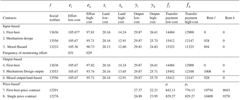
Table 1 shows parameter values and functional forms. The results in Table 2 show that where there is perfect information the regulator can achieve the same level of efficiency with an input contract (contract 1) and an output contract (contract 3). In the case of hidden land productivity, an input contract (contract 2) is slightly more efficient than an output contract (contract 4). Mixed contracts (contract 5) which target land and output are as efficient at addressing adverse selection as an input contract and can also induce a farmer to supply an optimal level of effort. This is an interesting result that holds trivially for the case of two inputs but in more complex policy settings may suggest that regulators should consider targeting more observable variables, which then provides an indirect incentive to manage inputs that are unobservable.

Table 3 here

an emphasis upon the ability of the regulator to estimate the non-market and market values of ES outputs as the price should be set relative to the ES value.

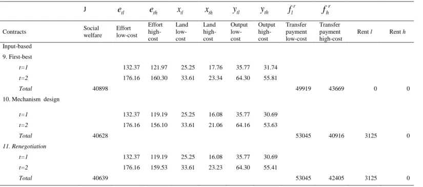
Table 3 gives results for the two-period input-based commitment model. The first-best solution (contract 9) provides a benchmark. Notice that the inputs increase in period two as the increase in the ecosystem asset raises their marginal products. The mechanism design solution (contract 10) reduces land and effort input for the high cost type. The renegotiation proof contract (contract 11) offers the mechanism design menu for both periods in the first period, but also implies that any renegotiation in the second cannot make farmers worse off. The solution shows that there is a modest increase in social welfare from this contract relative to the mechanism design contract. The rent of the l-type farmer is the same as that for

mechanism design and the high cost type switches to a first best level of land and effort given the ecosystem asset at the end of the first period. It is for this reason that the input levels are slightly less than for the first best.

5

Conclusions

In their assessment of European agri-environmental policy the European Court of Auditors (2011) conclude: “The Court found that the objectives determined by the Member States are numerous and not specific enough for assessing whether or not they have been achieved. … In

particular, very little information was available on the environmental benefits of

agri-environment payments. (European Court of Auditors, 2011, p7).

This paper identified a series of results that offer insights into the problems inherent in such a policy design process. First, with perfect information about farm type, the regulator is

measure the ES output and contract on it, then they can provide an incentive for an optimal level of the unobservable effort and informational rent. Result 4 shows that contracting on output eliminates the requirement for explicit effort monitoring.

A price-based contract that pays on ES output is attractive in terms of its administrative requirement as it only requires output monitoring. However, fixed price contracts are relatively costly to the regulator as they pay more rent to farmers (Hanley et al, 2012; Armsworth et al, 2012).

Results for multi-period adverse selection and renegotiation are complex and are approached here by assuming regulator commitment and only allowing Pareto improving renegotiation in the second period. This is appropriate in many contracts for ecosystem services, such as the native bush example, where significant gains to society derive from long term protection. Spot contracting, especially where paying on inputs only, is usually not optimal as it can lead to cycles of ecosystem asset appreciation and depreciation if there are gaps in the contract (Iossa and Rey, 2015). The practical implications of the results here are that in a multi-period contract setting, even if the contracts are on inputs, it is advisable to measure output as well as imposing an additional condition for recontracting. The duration of the contract stages is also important. There may be a case for a short initial period (say 3 years in the empirical example described above) that allows the farmer to signal to the regulator their type before the

regulator engages in Pareto improving renegotiation. This renegotiation sets up a long term contract (over 10 years, for instance) with a condition on renegotiation at the end of the second period.

Our results have been obtained by analysis of simplified models combined with a simulation of an actual policy setting. There are limitations to this approach and there is a requirement for further research into more complex settings, especially those relating to repeated

References

Anthon S, Garcia S, Stenger A (2010) Incentive contracts for Natura 2000 implementation in forest areas. Environmental and Resource Economics 46(3): 281–302

Armsworth P, Acs S, Dallimer M, Gaston K, Hanley N, Wilson P, (2012) The costs of simplification in conservation programmes. Ecology Letters, 15(5): 406–414

Balmford A, Green, R, Phalan B (2012) What conservationists need to know about farming. Proceedings of the Royal Society B: Biological Sciences 279(1739): 2714-2724 Barbier EB (2013). Wealth accounting, ecological capital and ecosystem services.

Environment and Development Economics 18(2): 133–161.

Baron, DP, (1985) Non-cooperative regulation of a non-localized externality. The RAND Journal of Economics, 16(4): 553-568

Bateman IJ, Mace GM,· Fezzi C, Atkinson G, Turner K (2011) Economic analysis for ecosystem service assessments. Environmental and Resource Economics 48(2):177– 218

Burton M, Zahedi J, White B (2012) Public Preferences for Timeliness and Quality of Mine Site Rehabilitation The Case of Bauxite Mining in Western Australia. Resources Policy 37(1):1-9

Burton RJF, Schwarz, G (2013) Result-oriented agri-environmental schemes in Europe and their potential for promoting behavioural change. Land Use Policy, 30(1): 628-641

Campbell HF, Bond KA (1997) The cost of public funds in Australia Economic Record 73(220): 22-34

Derissen S, Quaas M (2013) Combining performance-based and action-based payments to provide environmental goods under uncertainty. Ecological Economics 85: 77-84 European Court of Auditors (2011) Is agri-environment support well designed and managed?

European Court of Auditors, Luxembourg

Ferraro PJ (2008) Asymmetric information and contract design for payments for environmental services. Ecological Economics 65: 810-821

Gibbons JM, Nicholson E, Milner-Gulland, EJ, Jones, JPG (2011) Should payments for biodiversity conservation be based on actions of results? Journal of Applied Ecology, 48, 1218-1226

Hanley N, Banerjee S, Lennox G, Armsworth P, (2012) How should we incentivise private landowners to “produce” more biodiversity? Oxford Review of Economic Policy28 (1): 93-113

Hart O; Moore, J (1988) Incomplete contracts and renegotiation. Econometrica 56(4): 755-785

Herzfeld T, Jongeneel, RA (2012) Why do farmers behave as they do? Understanding compliance with rural, agricultural, and food attribute standards. Land Use Policy 29(1): 250-260

Hueth B, Melkonyan, T (2004) Multi-tasking, identity preservation, and contract design in agriculture. American Journal of Agricultural Economics 86(3): 842-847

Iossa E; Martimort D (2015) the simple microeconomics of public-private partnerships. Journal of Public Economic Theory 17(1): 4-48.

Kuhfuss L., R. Préget, S. Thoyer, N. Hanley, P. Le Coent and M. Désolé (2015)Nudges, social norms and permanence in
agri-environmental schemes . Discussion Papers in Environmental Economics 2015/15, University of St Andrews.

Laffont J-J, Tirole J (1993) A theory of incentives in procurement and regulation. MIT Press, Cambridge Mass

Laffont J-J, Tirole J, (1990) Adverse selection and renegotiation in procurement. Review Of Economic Studies 75 597–626.

Laffont J-J, Tirole J, (1988) The dynamics of incentive contracts. Econometrica 56(5): 1153-1175

Laffont, J-J, Martimort D, (2002) The theory of incentives: the principal-agent model Princeton University Press, Princeton, NJ

Lau LJ, (1976) Characterization of normalized restricted profit function. Journal of Economic Theory 12(1), 131-163

MacKenzie IA, Hanley N, Kornienko T, (2008) The optimal initial allocation of pollution permits: a relative performance approach. Environmental and Resource Economics, 39 (3): 265-282

Mäler K-G, Aniyar S, and Jansson Å (2009) Accounting for ecosystems. Environmental and Resource Economics 42(1): 39–51

Mas-Colell A. Whinston MD, Green, JR (1995) Microeconomic theory Oxford University Press, New York

Melkonyan T, Taylor M, (2013) Regulatory design for agroecosystem management on public rangelands. American Journal of Agricultural Economics 95(3): 606-627

Miteva D, Pattanayak S, and Ferraro P, (2012) Evaluation of biodiversity policy instruments. Oxford Review of Economic Policy, 28 (1): 69-92

Moxey A, White B, Ozanne A, (1999) Efficient contract design for agri-environment policy. Journal of Agricultural Economics 50(2): 187-202

Myers N, Mittermeier RA, Mittermeier CG, da Fonesca GAB and Kent J (2000) Biodiversity hotspots for conservation priorities. Nature 403(4): 853-858

Ozanne A, White B (2007) Equivalence of input quotas and input charges under asymmetric information in agri-environmental schemes. Journal of Agricultural Economics 58(2): 260-268

Prober SM, Smith FP (2009) Enhancing biodiversity persistence in intensively used

agricultural landscapes: A synthesis of 30 years of research in the Western Australian wheatbelt. Agriculture Ecosystems & Environment 132(SI): 173-191

Rey P, Salanie, B., (1990) Long-term, short-term and renegotiation - on the value of commitment in contracting. Econometrica 58(3): 597-619

Rey P, Salanie, B., (1996) On the value of commitment with asymmetric information. Econometrica 64(6): 1395-1413

Tirole J, (1999) Incomplete contracts: where do we stand? Econometrica, 67(4): 741-81 White B (2002) Designing voluntary agri-environmental policy with hidden information and

hidden action. Journal of Agricultural Economics. 53(2): 353-360

White B (2005) An Economic Analysis of Ecological Monitoring. Ecological Monitoring 189(1): 241-251

White B, Sadler, R (2012) Optimal conservation investment for a biodiversity-rich

Wu, JJ Babcock, BA (1996) Contract design for the purchase of environmental goods from agriculture. American Journal of Agricultural Economics, 78(4): 935-945

Appendix 1 Input-based contracts asymmetric information

The analysis of the theoretical model is greatly simplified by the fact that the IC for the l-type

farm and the IR constraint for the h-type farm are the only constraints that are binding Following Laffont and Tirole (1993, p59) The incentive compatibility constraint for the low cost farmer (IC-l) is:

( ( e, ) ( x, )) ( ( e, ) ( x, ))

l e l x l l h e h x l h

f  c  e c  x  f  c  e c  x (A1)

The individual rationality constraint for the h-type (IR-h) f_h( (c_e e,e_h)c_x(_hx,x_h))0

implies:

( ( e, ) ( x, )) ( ( e, ) ( x, )) ( ( e, ) ( x, )) 0

l e l x l l e h x h h e h x l h

f  c  e c  x  c  e c  x  c  e c  x 

As fh is at least ( ( , ) ( , ))

e x

e h x h h

c  e c  x , Thus we can ignore the IR-l constraint as it is implied by IC-l

If we now optimize (15) with respect to IC-l and IR-h it is possible to check that IC-h is satisfied from the first order conditions (17) and (18), x_l x_h and e_l e_h

If we restate the IC-l constraint:

(( ( , ) ( , )) ( ( , ) ( , ))

( , ) ( , )

e x e x

l h e h x l h e h x h h

x x

h x l h x h h

r r c e c x c e c x

r c x c x

   

 

    

  

Where r is the rent_i The IC-h is:

(( ( e, ) ( x, )) ( ( e, ) ( x, )) ( x, ) ( x, )

h l e l x h l e l x l l l x h l x l l

r  r c  e c  x  c  e c  x  r c  x c  x .

Bringing the constraints together:

0 ( ( x, ) ( x, )) ( x, ) ( x, )

x h h x l h x h l x l l

c  x c  x c  x c  x

The assumption that the IC-h constraint is implied by the IR-h and IC-l constraints holds as long as c'''_x(_ix, )x_i 0

Appendix 2 Equivalency between mixed contracts and second-best input-based contracts

The regulator maximizes:





, , ( , ( , )) ( , ( , )) ( , )- ,

i i i

e x

i i i i i e i i i x i i

x y f i

Maximum



Subject to the participation for the high-cost type

( e, ( , )) ( x, ) 0

h e h h x h h

f c  e x y c  x 

and incentive compatibility constraint for the low cost type:

( e, ( , )) ( x, ) ( e, ( , )) ( x, )

l e l l x l l h e h h x l h

f c  e x y c  x  f c  e x y c  x

Both constraints enter as equalities. The four first order conditions for xl, yl, xh, yhare:

' '

(1 ) ( , )+(1 ) ( , ( , )) e

e

l l l l

x e

x l i e i i x

e x x

c x c e x y

v g g         (A21) '

(1 ) ( , ( , )) l

e

e i i

e

c e x y

v g     (A22) ' ' ' ' ' '

( , )+ ( , ( , )) e ( / )( ( , )

( ( , ) ( , ( , )) e ( , ( , )) e )

e

h

h h

h h h

x e x

x h h e i i x h x h h

x e e

l x l h e h h x l e h h x

e x x

c x c e x y c x

c x c e x y c e x y

v g g                _{  }      (A23) ' ' '

(1 ) ( , ( , ))

( ( , ( , )) ( , ( , ))) h

e

e e

e h h l

e h h e h h

e h

c e x y

v c e x y c e x y

g

   _{ }





First we establish that the low cost farmer selects the first-best solution. Rearrange (A22) to give:

'

(1 ) ( , ( , )) l

e

e e i i

vg   c  e x y (A25)

and (A22) to give:

' '

( e ) (1 ) ( , )+(1 ) ( , ( , )) e

l l l l

x e

e x x x l i e i i x

v g g   c  x  c  e x y (A26)

Substituting for l e vg :

' ' '

(1 ) ( , ( , )) e (1 ) ( , )+(1 ) ( , ( , )) e

l l l

e x e

e i i x x x l i e i i x

c e x y vg c x c e x y

     

    

This simplifies to:

'

(1 ) ( , ) l

x

x x l i

vg   c  x

Establishing that the solution is identical to the optimal solution to the input-based contract On the basis of (A24) effort is also identical.

The area and effort for the high cost farmer can also be shown to be the same as for the input-based contract. From (A24) the last term is zero as the effort costs are identical and

rearranging:

'

(1 ) ( , ( , )) h

e

e e h h

vg   c  e x y (A27)

Rearranging (A23) and substituting in (A27) adding and subtracting '

( x, )

x h h

c x

  to the rhs and rearranging:

' ' ' '

' ' ' '

(1 ) ( , ( , )) e (1 ) ( , ) ( , )+ ( , ( , )) e ( / )( ( , ) ( ( , ) ( , ( , )) e ( , ( , )) e )

h h h

h h

e x x e

e h h x x x h h x h h e h h x

x x e e

h x h h l x l h e h h x l e h h x

c e x y vg c x c x c e x y

c x c x c e x y c e x y

      

       

     

Using the fact that '( , ( , )) e '( , ( , )) e '( , ( , )) e

h h h

e e e

e i i x l e i i x h e i i x

c  e x y  c e x y c  e x y

' ' '

' ' '

(1 ) ( , ( , )) e (1 ) ( , )+(1+ ) ( , ( , )) e

( / )( ( , ) ( , ) ( ( , ))

h h h

e x e

e h h x x x h h e i i x

x x x

h h x h h x h h l x l h

c e x y vg c x c e x y

c x c x c x

     

      

    

  

This simplifies to:

' ' '

(1 ) ( , )+( / )( ( , ) ( ( , ))

h

x x x

x x h h l h x h h l x l h

vg   c  x   c  x  c  x