An Elementary Study of Chaotic Behaviors in 1 D Maps

(1)

ISSN Online: 2327-4379 ISSN Print: 2327-4352

DOI: 10.4236/jamp.2019.75077 May 29, 2019 1149 Journal of Applied Mathematics and Physics

An Elementary Study of Chaotic Behaviors in

1-D Maps

Shah Abdullah Al Nahian

1

, Zakir Hosen

2

, Payer Ahmed

2

1_{Department of Mathematics, Bangladesh University of Engineering and Technology, Dhaka, Bangladesh} 2_{Department of Mathematics, Jagannath University, Dhaka, Bangladesh}

Abstract

In this article, we have discussed basic concepts of one-dimensional maps like Cubic map, Sine map and analyzed their chaotic behaviors in several senses in the unit interval. We have mainly focused on Orbit Analysis, Time Series Analysis, Lyapunov Exponent Analysis, Sensitivity to Initial Conditions, Bi-furcation Diagram, Cobweb Diagram, Histogram, Mathematical Analysis by Newton’s Iteration, Trajectories and Sensitivity to Numerical Inaccuracies of the said maps. We have tried to make decision about these mentioned maps whether chaotic or not on a unique interval of parameter value. We have performed numerical calculations and graphical representations for all para-meter values on that interval and have tried to find if there is any single value of parameter for which those maps are chaotic. In our calculations we have found there are many values for which those maps are chaotic. We have showed numerical calculations and graphical representations for single value of the parameter only in this paper which gives a clear visualization of chaotic dynamics. We performed all graphical activities by using Mathematica and MATLAB.

Keywords

Sensitivity, Trajectory, Numerical Inaccuracies, Orbit, Bifurcation, Cobweb Diagram

1. Introduction and Background

During the last few decades, dynamical system [1] has made long strides. Dy-namical system is the study of the long-term behavior of an evolving system. It is observed that in various models of economics, biology and various other sciences of the chaotic nonlinear dynamical system has made its presence felt. How to cite this paper: Al Nahian, S.A.,

Hosen, Z. and Ahmed, P. (2019) An Ele-mentary Study of Chaotic Behaviors in 1-D Maps. Journal of Applied Mathematics and Physics, 7, 1149-1173.

https://doi.org/10.4236/jamp.2019.75077

Received: March 19, 2019 Accepted: May 26, 2019 Published: May 29, 2019

http://creativecommons.org/licenses/by/4.0/

(2)

DOI: 10.4236/jamp.2019.75077 1150 Journal of Applied Mathematics and Physics

The phenomenon of chaos [2] has been studied extensively and it has attracted increasing interests from mathematicians, physicists, engineers, and so on. Since chaotic systems not only admit abundant complex and interesting dynamical behaviors but also have many potential practical applications, great efforts have been devoted to an investigation related to these systems.

Chaos is an interdisciplinary theory stating that within the apparent random-ness of chaotic complex systems, there are underlying patterns, constant feed-back loops, repetition, self-similarity, fractals, self-organization, and reliance on programming at the initial point known as sensitive dependence on initial con-ditions. The butterfly effect describes how a small change in one state a determi-nistic nonlinear system can result in large differences in a later state.

Chaos theory concerns deterministic systems whose behavior can in principle be predicted. Chaotic systems are predictable for a while and then “appear” to become random [3]. The amount of time that the behavior of a chaotic system can be effectively predicted depends on three things: How much uncertainty can be tolerated in the forecast, how accurately its current state can be measured, and a time scale depending on the dynamics of the system, called the Lyapunov time. Some examples of Lyapunov times are: chaotic electrical circuits. In chao-tic systems, the uncertainty in a forecast increases exponentially with elapsed time. Hence, mathematically, doubling the forecast time more than squares the proportional uncertainty in the forecast. This means, in practice, a meaningful prediction cannot be made over an interval of more than two or three times the Lyapunov time. When meaningful predictions cannot be made, the system ap-pears random. The most important aspects of chaotic behavior should appear in systems of lowest dimension. Thus, we would like in the first step to reduce as much as possible the dimension of state space. However, this quickly conflicts with the requirement of invertibility. On the one hand, it can be shown that maps based on a one-dimensional homeomorphism can only display stationary or periodic regimes, and hence cannot be chaotic. On the other hand, if we sacri-fice invertibility temporarily, thereby introducing singularities, one-dimensional chaotic systems can easily be found. In Mathematics, researchers deal with vari-ous maps to study the different qualitative features related to it. It is also seen that map with one critical point, is not too difficult to study. But a map with two critical points in symmetrical case which was first investigated by May [4][5]

who was motivated by a problem in genetics involving one locus with two alleles is little difficult. After the investigation, he concluded that cubic map could de-scribe the population dynamics of certain genetic groups. Also various research-ers contributed in the study of the cubic map [6]. Perhaps the two most fre-quently mentioned are the logistic map and the tent map. It is shown to be “universal” for a large family of maps. It is also shown in [7] that unimodal maps such as the sine map with negative Schwarzian derivative are chaotic (in many definitions on the word). The use of symbolic dynamics in analysis of maps on the unit interval can be seen in [8].

(3)

been developed in order to understand the dynamics of one-dimensional maps and have been applied to different maps. Griffin [9] discussed the bifurcation and entropy of one dimensional sine map, Hemanta [10] represents various bi-furcations in a cubic map, Hemanta and Sarmah [11] showed Lyapunov expo-nents and time series analysis of a chaotic cubic map. Hidayet and Mustafa [12]

represented the application of sine map in image cryptosystem; Xiuping [13]

showed the application of cubic map in image encryption. Ruman [14] discussed the dynamical behaviors of one-dimensional logistic map. Zakir [15]represents the dynamical behaviors of one-dimensional doubling map. The study aimed at finding whether the considered maps represent randomness in dynamics on a unique interval.

Yet despite these tremendous accomplishments and other remarkable ad-vances in our understanding of chaotic dynamics, there is still no clear discus-sion about the dynamics of sine and cubic maps in different chaotic approaches. These two maps are neglected yet. Such gaps in our understanding thrives us to find the dynamics of these two maps by analyzing more chaotic properties.

2. Basic Preliminaries

Dynamical Systems: Dynamical Systems is a branch of mathematics that at-tempts to understand processes in motion. The world’s weather is another sys-tem that changes in time as is the stock market.

Iteration: Iterate means to repeat a process over and over again. To iterate a functions means to evaluate the function over and over, using the output of the previous application as the input for the next.

Orbit: Given x0∈R₍x0 is called the seed or initial value of the orbit), we

define the orbit of x0 under f to be the sequence

( )

{

2

}

0, 1 0 , 2 0 , , n n 0 ,

x x = f x x = f x _ x = f x _ .

Fixed Points: Let f :R→R be a map. The point x0 is called fixed point if

( )

0 0

f x =x . Note that 2

( )

(

( )

)

( )

0 0 0 0

f x = f f x = f x =x , and in general

( )

0 0

n

f x =x _.

Periodic Orbit or Cycle: The point x0 is called periodic if f xn

( )

0 =x0 for

some n>0, where n is called the prime period of the orbit.

Chaotic Orbits: Over the last twenty five years, one of the major developments in mathematics is that many simple functions such as quadratic function of real variable exhibits orbits of incredible complexity called “sensitivity to initial con-ditions” and also called chaotic behavior.

Sensitivity on Initial Conditions: Mathematically, A continuous map :

f X →X _{has sensitive dependence on initial conditions if there exists} δ >0 such that, for any x X∈ and any neighborhood N x

( )

of x, there exist

( )

y N x∈ _, n≥0_{such that} _{d f x f y}

(

n

( )

, n

( )

)

_>

_δ

_{, where}

₍

_{X d}_,

₎

_{is a}

com-pact metric space.

Devaney’s Definition of Chaos (R. L. Devaney 1989):

(4)

DOI: 10.4236/jamp.2019.75077 1152 Journal of Applied Mathematics and Physics chaotic on X if f has the following three properties:

(C-1) Periodic points are dense in the space X. (C-2) f is topologically transitive.

(C-3) f has sensitive dependence on initial conditions.

Lyapunov Definition of Chaos: Consider the continuous and differentiable map f :R→R. Then f is said to be chaotic according to Lyapunov or L-chaotic if:

1) f is topologically transitive.

2) f has a positive Lyapunov exponent.

Trajectory: In dynamical systems, a trajectory is the set of points in state space that are the future states resulting from a given initial state. In a discrete dynam-ical system, a trajectory is a set of isolated points in state space. In a continuous dynamical system, a trajectory is a curve in state space.

Cubic Map: The Cubic map f :R→R is defined by _{f x}

( )

₌_x3 ₋_rx_.

Where r is the parameter, which is one of the simplest polynomial maps of the desired type. If r is restricted to the range 0≤ ≤r 3_then_f_{maps the interval}

[

1,1

]

x∈ − into itself and we will study the family f = fr for these parameter

values.

Sine Map: The Sine map is defined by f x

( )

=λsin

( )

πx ; x∈

[ ]

0,1 ,

[ ]

0,1

λ∈ _{, where} λ is the parameter value which lies between 0 and 1. This map is similar to the logistic map on the unit interval.

3. Theorems

3.1. Proposition

Show that the Cubic map _{f x}

( )

₌_x3₋_rx_{is chaotic in the interval} ₀_{≤ ≤}_r ₃_.

Proof: Here we discuss the Lyapunov exponent for the Cubic map

( )

3

f x =x −rx.

Consider two iterations of the Cubic map starting from two values of x which are close together. Let the two starting values be x0 and x0+δx0. These map

to x1 and x1+δx1, , xn+δxn . Expanding f x

( )

about xn we have

(

1

)

1

n n n

x f x x

δ = ′ ₋ δ ₋ . Assuming that δxn is sufficiently small. Hence the

sepa-ration of two trajectories after n steps, δxn is related to their initial separation

0

x

δ by 1

( )

0 0 n n i i

x _{f x} x

δ

− = ′

=

∏

. We expect that this will vary exponentially at large

n like

0 L r n x _e x

δ

= (Large n).

And so we define the Lyapunov exponent rL by

( )

1

1 lim n ln

L _n i

i

r f x

n

→∞ ₌ ′

=

∑

_{. If}

0

L

r > _{neighboring trajectories diverge from each other at large}_n_this corres-ponds to chaos. However if the trajectories converge to a fixed point or limit cycle they will get closer together, which corresponds to rL<0.

(5)

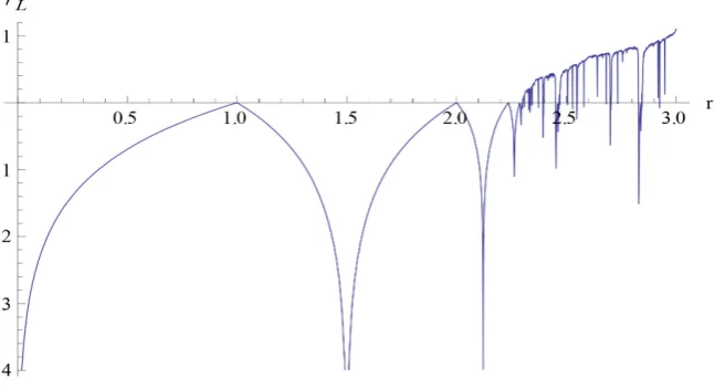
Below we calculate the Lyapunov exponent for some values of parameter r (not to be confused with the Lyapunov exponent rL). For r=2.56 we get

0.571265

L

r = _{. The positive value indicates that} r=2.56 is in a region of chaos. By contrast if we specify r=2.116 we get rL = −1.54957 which is a negative value, indicating that the trajectory of points x i_i

(

=0,1,2,_

)

converges to an attractor, which in this case we already know is a length of 2 limit cycle. Next lets plot the Lyapunov exponent for a range of values of r.

The main significance of Figure 1 is that one can easily distinguish the regions which are chaotic

(

rL >0

)

from the regions which tend to a fixed point or limit cycle

(

rL <0

)

. We see several points (the first is at r=1) where the Lyapunov exponent hits 0 and then goes negative again. These are the period doubling bi-furcations. Precisely at the period doubling point the system is at the limit of chaos, but then becomes non-chaotic when the period doubles. However, at the end of the period doubling regime, at r about 2.3024, rL crosses the axis and

the system enters a chaotic regime.

Note that for r in the range greater than the point where rL first goes

posi-tive, there are many regions where rL is negative, is known as “island of

stabil-ity” where the behavior is fixed point or limit cycle [16]. Notice that there are fine details no matter how much one expands the scale. We see that chaos emerges (i.e. rL >0) for r between 2.3024 and 2.8999. It is again become non chaotic for the values of r between 2.8999 and 2.985 then it enters into the chao-tic region again.

3.2. Proposition

Show that the Sine map f x

( )

=λsin

( )

πx _{is chaotic in the interval} 0≤ ≤λ 1_. Proof: Here we discuss the Lyapunov exponent for the Sine map

( )

sin

( )

π

f x =λ x _.

[image:5.595.211.535.532.708.2]

Consider two iterations of the Sine map starting from two values of x which are close together. Let the two starting values be x0 and x0+δx0. These map

(6)

to x1 and x1+δx1, , xn+δxn . Expanding f x

( )

about xn we have

(

1

)

1

n n n

x f x x

δ = ′ − δ − . Assuming that δxn is sufficiently small. Hence the

sepa-ration of two trajectories after n steps, δxn is related to their initial separation

0

x

δ _by 1

( )

0 0 n n i i x f x x

δ

− = ′

=

∏

. We expect that this will vary exponentially at large

n like

0 L n x _e x λ

δ

= .

(Large n) And so we define the Lyapunov exponent λL by

( )

1

1 lim n ln

L _n i

i f x n

λ

→∞ ₌ ′

=

∑

_{. If} λ >L 0 neighboring trajectories diverge from each

other at large n this corresponds to chaos. However if the trajectories converge to a fixed point or limit cycle they will get closer together, which corresponds to

0

L

λ < . Hence we can determine whether or not the system is chaotic by the sign of the Lyapunov exponent. Below we calculate the lyapunov exponent for some values of parameter λ (not to be confused with the Lyapunov exponent λL).

For λ=0.9 we get λ =L 0.354839. The positive value indicates that λ=0.9 is in a region of chaos. By contrast if we specify λ=0.55 we get

1.42149

L

λ = − _{which is a negative value, indicating that the trajectory of points}

(

0,1,2,

)

i

x i=  converges to an attractor, which in this case we already know is a length of 2 limit cycle. Next lets plot the Lyapunov exponent for a range of values of λ.

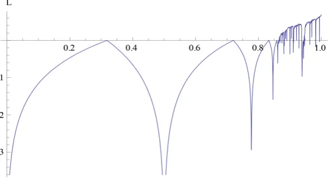
One can easily distinguish from Figure 2 the regions which are chaotic

[image:6.595.213.536.531.709.2]

(

λL>0

)

from the regions which tend to a fixed point or limit cycle

(

λL <0

)

. We see several points (the first is at a=0.31849) where the Lyapunov exponent hits 0 and then goes negative again. These are the period doubling bifurcations. Precisely at the period doubling point the system is at the limit of chaos, but then becomes non-chaotic when the period doubles [16]. However, at the end of the period doubling regime, at λ_{about 0.865,} λ_L_{crosses the axis and the} system enters a chaotic regime. Notice that there is fine detail no matter how

(7)

much one expands the scale. We see that chaos emerges (i.e. λ >L 0) for λ between 0.8655 and 0.8660. It is again become non chaotic for the values of λ between 0.8810 and 0.8825 then it enters into the chaotic region finally.

4. Theoretical Foundation

In this article we have not established new theorem but we have analyzed new chaotic properties for two maps named Sine map, Cubic map graphically and numerically based on the chaotic properties established by renowned mathema-ticians R. L. Devaney, Henry Poincare, Edward Lorentz and some of modern re-searchers. These strong properties show that these maps are chaotic clearly.

5. Result Discussion

5.1. Behavior of the Maps Taking Initial Seeds

Cubic map: In this section we iterate the cubic map _{f x}

( )

₌_{x rx}3₋ _{for the}

following r and x0 values (initial seeds) and investigate the dynamical behavior

of the given function f x

( )

considering the following case: r=2.9 1) For x0=0.30, The orbit is:

{

0.30, 0.84,1.84,0.93, 1.89, 1.30,1.57, 0.68,1.66,− − − − _

}

2) For x0=0.35, The orbit is:

{

0.35, 0.97,1.90,1.35, 1.44,1.16, 1.79, 0.59,1.51,− − − − _

}

{

0.45, 1.21,1.73,0.17, 0.48,1.30, 1.56,0.68, 1.67,− − − − _

}

{

0.50, 1.32,1.51, 0.91,1.88,1.23, 1.69,0.05, 0.17,− − − − _

}

Do you see any pattern? Obviously not. There is no initial seed for which the orbit forms any cycle and forms any kind of patterns. The orbits approach ran-domly. The initial seeds 0.30, 0.35, 0.45 and 0.50 are neither fixed/periodic points nor eventually fixed/periodic points of f x

( )

. We conclude that the dy-namical behavior [17] of the given function for r=2.9 is chaotic.

Sine map: Now we want to investigate the behavior of sine map for λ∈

[ ]

0,1 _. For this we iterate the Sine map f x

( )

=λsin

( )

πx for the following λ and

0

x values (initial seed) and we investigate the dynamical behavior of the given function f x

( )

considering the following case: Taking λ=0.95;

{

0.30,0.77,0.63,0.87,0.37,0.88,0.35,0.84,0.44,

}

{

0.35,0.84,0.44,0.93,0.19,0.55,0.94,0.18,0.52,

}

{

0.45,0.94,0.18,0.51,0.95,0.15,0.44,0.93,0.20,

}

{

0.50,0.95,0.15,0.92,0.22,0.60,0.89,0.30,

}

(8)

0.35, 0.45 and 0.50 are neither fixed/periodic points nor eventually fixed/periodic points of f x

( )

. We conclude that the dynamical behavior of the given function is chaotic [18] for λ=0.95_.

5.2. Orbit Analysis of the Maps

Cubic map: Here we want to observe closely the behavior of the orbit graphi-cally for given cubic map _{f x}

( )

₌_{x rx}3₋ _{. Consider} _r₌_2.6_{to make a decision}

about the dynamical behavior of the orbits graphically for the following initial seeds.

Taking different initial seeds graphically we see from Figure 3 and Figure 4

that the orbit of given dynamical system changes its nature randomly. So we can conclude that the given Cubic map is chaotic for some values of r∈

[ ]

0,3 .

Sine map: Now we want to perform same analysis for Sine map to do this we observe closely the behavior of the orbit graphically for given Sine map

( )

sin

( )

π

f x =λ x _{considering different} x₀ values (initial seeds). Take λ=0.95 and observe the dynamical behavior of the orbits graphically for the following initial seeds.

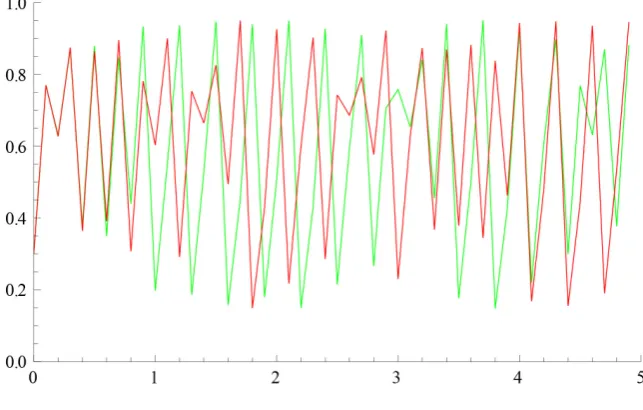
Taking different initial seeds from Figure 5 and Figure 6 graphically we see that the orbit of given dynamical system changes its nature randomly. So the given Sine map is chaotic for some values of λ∈

[ ]

0,1 .

5.3. Sensitivity Analysis of the Maps

We want to check the difference of the orbit by taking two neighbouring initial seeds. We first define the function governing the system and then calculate the distance between two orbits for the considered neighbouring initial seeds. Here we will consider 100 iteration and calculate the distance between two orbits. Af-ter that we will analyze whether the function is chaotic or not.

Cubic map: In this passage we want to analyze the sensitivity of Cubic map

( )

3

f x =x rx− . Taking r=2.6 and two neighboring initial seeds x0=0.30

[image:8.595.215.532.537.703.2]

and x0=0.31 we get the following table.

(9)

[image:9.595.213.537.75.238.2] [image:9.595.210.534.284.451.2]

DOI: 10.4236/jamp.2019.75077 1157 Journal of Applied Mathematics and Physics Figure 4. Consider initial seed x0=0.35.

[image:9.595.211.536.482.653.2]

Figure 5. Consider initial seed x0=0.30.

Figure 6. Consider initial seed x0=0.35.

(10)

[image:10.595.208.537.89.312.2]

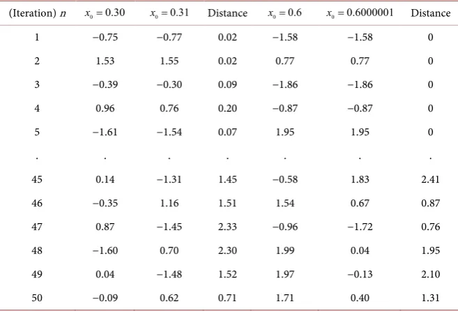
DOI: 10.4236/jamp.2019.75077 1158 Journal of Applied Mathematics and Physics Table 1. Sensitivity analysis of cubic map.

(Iteration) n x0=0.30 x0=0.31 Distance x0=0.6 x0=0.6000001 Distance

1 −0.75 −0.77 0.02 −1.58 −1.58 0

2 1.53 1.55 0.02 0.77 0.77 0

3 −0.39 −0.30 0.09 −1.86 −1.86 0

4 0.96 0.76 0.20 −0.87 −0.87 0

5 −1.61 −1.54 0.07 1.95 1.95 0

. . . .

45 0.14 −1.31 1.45 −0.58 1.83 2.41 46 −0.35 1.16 1.51 1.54 0.67 0.87 47 0.87 −1.45 2.33 −0.96 −1.72 0.76 48 −1.60 0.70 2.30 1.99 0.04 1.95 49 0.04 −1.48 1.52 1.97 −0.13 2.10 50 −0.09 0.62 0.71 1.71 0.40 1.31

We can say that the given Cubic map is chaotic for r=2.6 according to the sensitivity to initial condition. Here we have only taken the values up to 2 de-cimal places and analyzed the orbits from the 1st_{to 100}th_{positions. From this} analysis we have already reached to our goal which we sat before. We found that given function is chaotic for some values of r∈

[ ]

0,3 . The graphical representa-tion of the above sensitivity analysis is shown below.

Is there any clear message for us in Figure 7 and Figure 8? Yes. In Figure 7

the orbits for two considered initial seeds are same up to 7th_{iteration than go far} from each other. In Figure 8 the orbits for two considered initial seeds are same up to 18th_{iteration than separate. The orbits of the given Cubic map for two sets} of neighbouring initial seeds do not coincide with each other. Two orbits are scattered. They show randomness in distance from each other and go far from each other after a large number of iteration. In above Figures red line represents the orbit of x0=0.30 and 0.6 and green line represents the orbit of x0=0.31

and 0.6000001.

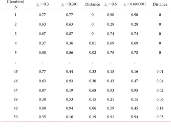
Sine map: In this passage we want to analyze the sensitivity of Sine map

( )

sin

( )

π

f x =λ x . Taking λ=0.95 and two neighbouring initial seeds

0 0.600

x = _and x₀=0.601_{we get the following table.}

We see from Table 2 that the distance between the two orbits is bouncing between 0 and 1 in an apparent erratic manner. This type of behavior tells us the system is chaotic. We can conclude that the given Sine map is chaotic [19] for

0.95

λ= according to the sensitivity to initial condition.

Here we have only taken the values up to 2 decimal places and analyzed the orbits from the 1st_{to 100}th_{positions considering neighbouring initial seeds}

0 0.3

x = , x0=0.301_and x0=0.6, x0 =0.6000001. From this analysis we can

(11)

[image:11.595.207.535.68.442.2]

DOI: 10.4236/jamp.2019.75077 1159 Journal of Applied Mathematics and Physics Figure 7. Two nearby seeds x0=0.30,0.31.

[image:11.595.204.539.485.735.2]

Figure 8. Two nearby seeds x0=0.6,0.6000001.

Table 2. Sensitivity analysis of Sine map. (Iteration)

N x0=0.3 x0=0.301 Distance x0=0.6 x0=0.6000001 Distance

1 0.77 0.77 0 0.90 0.90 0

2 0.63 0.63 0 0.28 0.28 0

3 0.87 0.87 0 0.74 0.74 0

4 0.37 0.36 0.01 0.69 0.69 0

5 0.88 0.86 0.02 0.78 0.78 0

. . . .

45 0.77 0.44 0.33 0.15 0.16 0.01

46 0.63 0.93 0.30 0.43 0.47 0.04

47 0.87 0.19 0.68 0.93 0.95 0.02

48 0.38 0.53 0.15 0.21 0.15 0.06

49 0.88 0.94 0.06 0.59 0.45 0.14

(12)

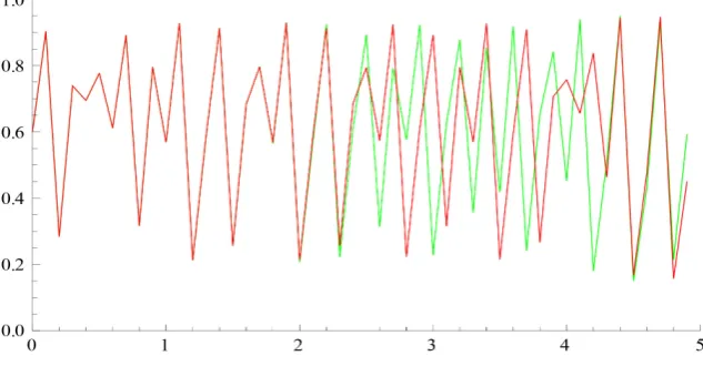
From Figure 9 we see that the orbits for two considered initial seeds are same up to 4th_{iteration than go far from each other. In}_{Figure 10}_{the orbits for two} considered initial seeds are same up to 22th_{iteration than separate. The orbits of} the given Sine map for two sets of neighbouring initial seeds do not coincide with each other. They show randomness in distance from each other and go far from each other after a large number of iteration.

In above Figures red line represents the orbit of x0 =0.3 and 0.6 and green

line represents the orbit of x0=0.301 and 0.6000001.

5.4. Time Series Analysis Graphically

Cubic map: The orbits listed in the numerical iteration part considering dif-ferent initial seeds seem to be wandering around the interval − ≤ ≤1 x 1_rather aimlessly. Let’s see if we can detect a pattern from the time series for one of these orbits. Here is the time series graph for the seed x0 =0.2,0.2001 with iteration

100 respectively.

Just when we think we are beginning to see a pattern in the above Figure 11

and Figure 12, the time series graphs begins to do something else and a new pattern emerges after some iteration we observe that there is no pattern in the above picture. This is called the unpredictability [20] which is another meaning of Chaos.

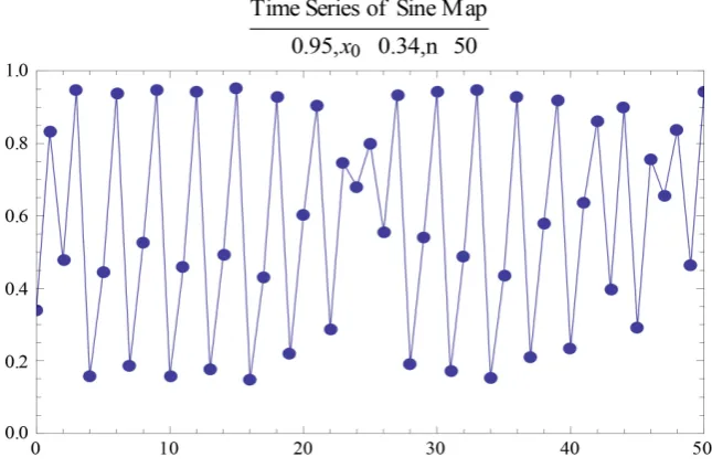
Sine map: The orbits of given Sine map seem to be wandering around the in-terval − ≤ ≤1 x 1_{rather aimlessly. Let’s see if we can detect a pattern from the} time series for one of these orbits. Here is the time series graph for the seed

0 0.34,0.2

x = _{with iteration 50, 100 respectively.}

[image:12.595.211.533.507.712.2]

From the above time series graph we see that there is no pattern and when we think for a pattern the graph in the Figure 13 and Figure 14 display some new shape. This graph approaches with erratic manner which we call as chaos.

(13)

[image:13.595.213.530.76.241.2] [image:13.595.209.534.271.484.2]

DOI: 10.4236/jamp.2019.75077 1161 Journal of Applied Mathematics and Physics Figure 10. For initial seeds x0=0.6,x0=0.6000001.

Figure 11. For r=3,x0=0.2,n=100.

[image:13.595.209.533.512.702.2]

(14)

[image:14.595.208.531.75.287.2]

DOI: 10.4236/jamp.2019.75077 1162 Journal of Applied Mathematics and Physics Figure 13. For λ=0.95,x0=0.34,n=50.

Figure 14. For λ=0.95,x0=0.2,n=100.

5.5. Cobweb Diagram

Analysis: While all of this vocabulary is helpful, a visual presentation of orbits helps solidify the concept. We call these diagram cobweb plots[18] and con-struct them as follows.

Let x0 be the seed of our orbit. In our plot we graph both our function

( )

f x and the line g x

( )

=x, in red. With these guidelines, we first trace a line, in black, from

(

x x0, 0

)

to

(

x f x0,

( )

0

)

, then from

(

x f x0,

( )

0

)

to

( ) ( )

(

f x0 ,f x0

)

(this is where plotting g x

( )

=x is useful). From there we can

trace a line to

(

( )

2

( )

)

0 , 0

f x f x , then to

(

2

( )

2

( )

)

0 , 0

f x f x and so on. With these plots, we can find _{f x}n

( )

_{for any}_n_{and perhaps more importantly, see}

[image:14.595.211.530.317.530.2]

(15)

Cubic map: With a basic understanding of cobweb plots, we can start to visu-al the behavior of cubic map _{f x}

( )

₌_{x rx}3₋ _{for larger values of}

_n

_.

We see that the orbit of 0.1 continues to hit new points. Figures 15-17 reveal that the orbit of x0 =0.1 under f seems to travel all over the interval

[

−1.5,1.5

]

_{. This phenomenon is called chaotic behavior. So we can say that the}

given Cubic map is chaotic for r=2.5.

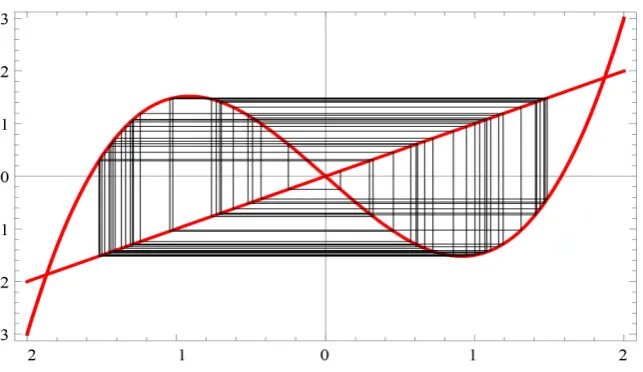
Sine map: Now we can start to analyze the behavior of sine map

( )

sin

( )

π

f x =λ x from cobweb plot for larger values of n.

The orbits still covering new ground. Figures 18-20 reveal that the orbit of

0 0.1

x = _under_f_{seems to travel all over the interval}

[

0.25,0.95

]

. This pheno-menon is called chaotic behavior. So we can say that the given Sine map is chao-tic for λ=0.9.

5.6. Histogram Analysis

Cubic map: Here we consider the cubic map _{f x}

( )

₌_{x rx}3₋ _{and investigate}

the dynamical behavior of the given function by analyzing the histogram image. From above histogram in Figure 21 we see that the variable values of the giv-en function fall into differgiv-ent bin or bucket [20] and each bin touches each other. The variable of the given function is scattered and hence the function is chaotic for r=2.6.

Sine map: Now we plot the histogram image of Sine map f x

( )

=λsin

( )

πx and investigate the dynamical behavior of the given function by analyzing the histogram image with the idea mentioned above.

[image:15.595.211.533.491.677.2]

From above histogram in Figure 22 again we see that the variable values of the given function fall into different bin or bucket [20] and each bin touches each other. The variable of the given Sine map is scattered and hence the func-tion is chaotic for some λ∈

[ ]

0,1 .

Figure 15. Represents the cobweb plot of x0=0.1 under the map

( )

3

f x =x rx− _with 2.5

(16)

DOI: 10.4236/jamp.2019.75077 1164 Journal of Applied Mathematics and Physics Figure 16. Represents the cobweb plot of x0 =0.1 under the map f x

( )

=x rx3−

with r=2.5 up to 100 iterations.

Figure 17. The cobweb plot of x0=0.1 under the map f x

( )

=x rx3− with r=2.5

up to 100 iterations.

Figure 18. Represents the cobweb plot of x0=0.1 under the map f x

( )

=λsin

( )

πx

[image:16.595.210.539.70.235.2] [image:16.595.210.539.287.459.2] [image:16.595.210.540.508.678.2]

(17)

DOI: 10.4236/jamp.2019.75077 1165 Journal of Applied Mathematics and Physics Figure 19. Represents the cobweb plot of x0=0.1 under the map f x

( )

=λsin

( )

πx

with λ =0.9 up to 100 iterations.

Figure 20. The cobweb plot of x0 =0.1 under the map f x

( )

=λsin

( )

πx with

0.9

[image:17.595.208.538.70.245.2]

λ= up to 500 iterations.

[image:17.595.212.539.291.460.2] [image:17.595.208.535.494.730.2]

(18)

[image:18.595.211.530.74.267.2]

DOI: 10.4236/jamp.2019.75077 1166 Journal of Applied Mathematics and Physics Figure 22. Histogram of sine map for λ =0.90.

5.7. Mathematical Analysis by Newton’s Iteration

Cubic map: Consider the cubic map _{f x}

( )

₌_{x rx}3₋ _{and choose}_r₌_2.6_.

The Newton’s iteration function [21] associated with f x

( )

is defined by

( )

_{( )}

₃32 2.6_2.6 3 3 2.6₃ 2 _2.63 2.6 ₃ 22 3_2.6

f x x x x x x x x

N x x x

f x x x x

− − − +

= − = − = =

′ − − −

Using the Mathematica program, we get the following orbits for the points 3.90, 3.92, 3.94, 3.96, 3.98,3.90,3.92,3.94,3.96

x= − − − − − and 3.98 under N.

3.90→2.13→1.49→1.79→1.50→1.76→1.51 1.75→ →1.52→1.73→1.52→1.72→1.53 3.92→2.14→1.49→1.79→1.50→1.76→1.51 1.74→ →1.52→1.73→1.53→1.72→1.53 3.94→2.15→1.49→1.78→1.51 1.76→ →1.51 1.74→ →1.52→1.73→1.53→1.72→1.53 3.96→2.16→1.50→1.78→1.51 1.76→ →1.51 1.74→ →1.52→1.73→1.53→1.72→1.53 3.98→2.17→1.50→1.78→1.51 1.76→ →1.52→1.74→1.52→1.73→1.53→1.72→1.53 Thus we see that orbit of any positive or negative real point under N makes a cycle of period-2 for all real value of r.

Sine map: Now we consider the Sine map f x

( )

=λsin

( )

πx _{and choose} 0.9

λ= . The Newton’s iteration function associated with f x

( )

is defined by

( )

_{( )}

sin

( )

_{( )}

π sin

( )

_{( )}

π tan

( )

π

cos π cos π

f x x x

N x x x x x x

f x x x

λ λ

= − = − = − = −

′

Using similar program we get the following orbits for the points 3.90, 3.92, 3.94, 3.96

x= − − − − under N.

0.6→1.58→2.82→3.02→2.99→ → → → →3 3 3 3 3 1.2→0.97→ → → → → →1 1 1 1 1 1

1.8→2.03→1.99→ → → → →2 2 2 2 2

2.4→1.42→0.17→ −0.02→ → → → →0 0 0 0 0

(19)

con-DOI: 10.4236/jamp.2019.75077 1167 Journal of Applied Mathematics and Physics

verges to a fixed point. Here in this analysis we notice that there are infinitely many fixed points for all real value of λ. For different initial values we get new fixed points whether we increase or decrease the initial value in any scale [21]_.

5.8. Sensitivity to Numerical Inaccuracies

Cubic Map: For some values of the parameter r, the Cubic model

3 1

n n n

x+ =x −rx is very sensitive to numerical inaccuracies. To see this, we calcu-late 100 values from the model with r = 3, first by using normal decimal num-bers and then by using high-precision numnum-bers. In the latter case, we start with numbers that have a precision of 65 digits:

(

)

(

)

3

values1 NestList # 3# &,0.02,40 ;

values2 NestList # 3# &,0.02`55,40

 

= _ − _

 

= _ − _

Values corresponding to values 2 are thick. From approximately iteration 37 on, the values differ greatly. In calculating values 2, we started with numbers having 55 digits of precision. During the calculation, many digits were lost so that the last value −0.7512329 only has a precision of approximately 7.25962. Look at some elements of values 2.

Thus, we know that all the digits of values2 are correct. This means that the values in values1 are incorrect from approximately iteration 37 on. This demon-strates the sensitivity to numerical inaccuracies of the Cubic map for some val-ues of the parameter r. Thus, if we calculate long sequences from the Cubic function, it is important to use a high enough precision during the calculation. From the plot of values2 in Figure 23, we see that the series behaves quite chaotically. It is known that chaotic models are very sensitive to numerical in-accuracies.

Sine map: For some values of the parameter λ , the Sine map

( )

1 sin π

n n

x₊ =λ x is very sensitive to numerical inaccuracies. To see this, we calculate 90 values from the model with λ=1, first by using normal decimal numbers and then by using high-precision numbers. In the latter case, we start with numbers that have a precision of 35 digits:

( )

(

)

(

( )

)

val1 NestList sin # &,0.01,90 ; val2 NestList sin # &,0.01`35,90 ;= _

π

_ = _

π

_

Values corresponding to val2 are thick. From approximately iteration 53 on, the values differ greatly. In calculating val2, we started with numbers having 35 digits of precision. During the calculation, many digits were lost so that the last value 0.1282 only has a precision of approximately 9.68. Look at some elements of val2.

(20)

[image:20.595.210.535.76.176.2]

DOI: 10.4236/jamp.2019.75077 1168 Journal of Applied Mathematics and Physics Figure 23. Sensitivity to numerical inaccuracies of the cubic map.

in Figure 24, again we see that the series behaves quite chaotically. It is known that chaotic models are very sensitive to numerical inaccuracies.

5.9. Trajectories of the Maps

Cubic map: Write the equation in the form

(

3

)

1

n n n n n

y+ −y = y ry− −y and

draw the trajectories for different r∈

[ ]

0,3 . We first calculate a solution set by starting from various points and iterating the equation n times. The starting points are chosen between y01 and y02 in steps of dy0. When r = 1.5, we

get the following trajectories.

The trajectory in Figure 25 seems to form a cycle of two points. In Figure 26

the trajectory appears to be chaotic. Thus from the trajectory [22] of Cubic map we can make decision that it is chaotic for some r∈

[ ]

0,3 .

Sine map: Now we want to perform same analysis for sine map which we performed above for cubic map. To do this we first write the equation in the form xn+1−xn =λsin

( )

πxn −xn and plot the trajectories for different value of

[ ]

0,1

λ∈ . We first calculate a solution set by starting from various points and iterating the equation n times. The starting points are chosen between x01 and

02

x in steps of dx0. When λ=0.6, we get the following trajectories.

The trajectory in Figure 27 seems to approach to a fixed point. In Figure 28

the trajectory appears to be chaotic. From the above trajectories of Sine map we can find that it is chaotic for some λ∈

[ ]

0,1 _.

5.10. Bifurcation Diagram

Cubic map: A bifurcation diagram is a visual summary of the succession of period-doubling produced as r increases. The next figure shows the bifurcation diagram of the Cubic map, r along the x-axis. For each value of the system is first allowed to settle down and then the successive values of x are plotted for a few hundred iterations.

(21)

[image:21.595.210.536.68.208.2]

DOI: 10.4236/jamp.2019.75077 1169 Journal of Applied Mathematics and Physics Figure 24. Sensitivity to numerical inaccuracies of the sine map.

Figure 25. Trajectory for r = 1.5.

[image:21.595.211.537.240.569.2]

Figure 26. Trajectory for r = 2.6.

Figure 27. Trajectory for λ =0.6.

(22)

[image:22.595.210.538.71.304.2]

DOI: 10.4236/jamp.2019.75077 1170 Journal of Applied Mathematics and Physics Figure 28. Trajectory for λ =0.9.

Figure 29. Bifurcation diagram of cubic map for 0≤ ≤r 3_.

Sine map: The next figure shows the bifurcation diagram of the Sine map, λ along the x-axis. For each value of the system is first allowed to settle down and then the successive values of x are plotted for a few hundred iterations.

We observe that for λ less than 0.3, all the points are plotted at zero in be-low Figure 30. Zero is the one point attractor for λ less than 0.3. For λ be-tween 0.3 and 0.72 (approximately), we still have one-point attractors, but the “attracted” value of x increases as λ increases, at least to λ=0.72. Bifurca-tions occur at λ=0.72, λ=0. 2,7 0.83,0.85,0 6.8 ,__{(approximately), etc.,} un-til just beyond 0.94, where the system is chaotic. However, the system is not chaotic for all values of r greater than 0.94. Here we can see some new lines ap-pear. For the non-chaotic parts of the diagram, these lines trace the values that x visits before settling into an oscillation. The windows of period three (at about

0.94

λ= _{), period four (at about} λ=0.85 _{), and period eight (at about} 0.86

λ= ) are clearly visible in the above diagram. The appearance and behavior of the bifurcation diagram is very similar to that of the logistic map, albeit with different parameter values. There is a good reason for this.

6. Socio-Economic Importance

(23)

[image:23.595.210.539.54.190.2]

DOI: 10.4236/jamp.2019.75077 1171 Journal of Applied Mathematics and Physics Figure 30. Bifurcation diagram of Sine map for 0≤ ≤λ 1.

is another area that has recently benefited from chaos theory. For over a hun-dred years, biologists have been keeping track of populations of different species with population models. Another biological application is found in cardiography. Fetal surveillance is a delicate balance of obtaining accurate information while being as non-invasive as possible.

In this paper we have worked on two real maps namely Sine and Cubic maps. These two maps have many uses in socio-economic sectors such as Sine map can be used in electricity, digital signals, sound systems, image encryptions etc. and cubic map can be used in traffic systems, in robotics, in computer science etc. To apply any map in any sector it is sufficient to know the nature or dynamics of that map otherwise the predictions will be wrong and the ultimate goal will not been obtained. We have tried to analyze the main dynamical properties of chaos which are essential for the new mathematics researchers. Then they will be able to apply the chaos in real life and will bring new revolutionary changes in the research fields of chaos which will open the new way of mathematical research.

7. Limitations

In this paper we have found a major limitation which is software problem while preparing Orbit analysis, Cobweb and bifurcations of Sine & Cubic map. First we have done these properties graphically using Mathematica 7.0 but it works very slowly and takes much time to show those graphs. The graphs are not clearly visualized for the software problem. Therefore Software version problem can be treated as our major limitation of our paper. Of course high speed super computer is very much needed to run those related programs quickly to show the graphs clearly.

8. Conclusion

(24)

Acknowledgements

I am deeply grateful those who have helped me this work in different ways.

Conflicts of Interest

The authors declare no conflicts of interest regarding the publication of this pa-per.

References

[1] Martelli, M. (1999) Introduction to Discrete Dynamical Systems and Chaos. John Wiley & Sons Inc., New York.https://doi.org/10.1002/9781118032879

[2] Gleick, J. (1987) Chaos: Making a New Science. Viking, New York.

[3] Boeing, G. (2016) Visual Analysis of Nonlinear Dynamical Systems: Chaos, Fractals, Self-Similarity and the Limits of Prediction. Systems, 4, 37.

https://doi.org/10.3390/systems4040037

[4] May, R.M. (1979) Bifurcations and Dynamical Complexity in Ecological Systems. Annals of the New York Academy of Sciences, 316, 517-529.

https://doi.org/10.1111/j.1749-6632.1979.tb29494.x

[5] May, R.M. (1980) Nonlinear Phenomena in Ecology and Epidemiology. Annals of the New York Academy of Sciences, 357, 267-281.

https://doi.org/10.1111/j.1749-6632.1980.tb29692.x

[6] Rogers, T.D. and Whitley, D.C. (1983) Chaos in the Cubic Mapping. Mathematical Modelling, 4, 9-25. https://doi.org/10.1016/0270-0255(83)90030-1

[7] Hussein, H.J.A. and Abed, F.S. (2012) On Some Dynamical Properties of Unimodal Maps. Pure Mathematical Sciences, 1, 53-65.

[8] Milnor, J. and Thurston, W. (1988) On Iterated Maps of the Interval. In: Alexander, J.C., Ed., Dynamical Systems, Lecture Notes in Mathematics, Springer, Berlin, Hei-delberg, 465-563.https://doi.org/10.1007/BFb0082847

[9] Griffin, J. (2013) The Sine Map.

https://people.maths.bris.ac.uk/~macpd/ads/sine.pdf

[10] Sarmah, H.K. and Das, M.C. (2014) Various Bifurcations in a Cubic Map. Interna-tional Journal of Advanced Scientific and Technical Research, 3, 827-846.

[11] Hemanta Kr., S., Ruma, S. and Das, N. (2010) Bifurcation and Lyapunov Exponent of a Chaotic Cubic Map. International Journal of Engineering Research and Appli-cations, 3, 93-106.

[12] Oğraş, H. and Türk, M. (2016) A Secure Chaos-based Image Cryptosystem with an Improved Sine Key Generator. American Journal of Signal Processing, 6, 67-76. [13] Yang, X., Min, L. and Xue, W. (2015) A Cubic Map Chaos Criterion Theorem with

Applications in Generalized Synchronization Based Pseudorandom Number Gene-rator and Image Encryption. Chaos: An Interdisciplinary Journal of Nonlinear Science, 25, Article ID: 053104.https://doi.org/10.1063/1.4917380

[14] Rumman, U., Tania, R.T. and Titu, M.A.S. (2013) Dynamical Behavior of Logistic Maps. International Journal of Computer Applications, 72, No. 12.

[15] Hosen, M.Z., Zillu, M.M. and Ahmed, P. (2018) Several Chaotic Approaches of One Dimensional Doubling Map. American Scientific Research Journal for Engineering, Technology and Sciences, 43, No. 1.

(25)

Lyapu-DOI: 10.4236/jamp.2019.75077 1173 Journal of Applied Mathematics and Physics

nov Exponents for Chaotic Logistic Maps. Journal of the Royal Statistical Society: Series B, 57, 439-452. https://doi.org/10.1111/j.2517-6161.1995.tb02038.x

[17] Devaney, R.L. (1989) An Introduction to Chaotic Dynamical Systems. Addison Wesley, Boston, MA.

[18] Alligwood, K.T., Sauer, T.D. and Yorke, J.A. (1996) Chaos: An Introduction to Dy-namical Systems. Springer-Verlag, New York.

[19] Ott, E. (1993) Chaos in Dynamical Systems. Cambridge University Press, Cam-bridge.

[20] Sprott, J.C. (2003) Chaos and Time-Series Analysis. Oxford University Press, New York.

[21] https://www.math.ubc.ca/~anstee/math104/newtonmethod.pdf

[22] Parker, T.S. and Chua, L.O. (1989) Practical Numerical Algorithms for Chaotic Systems. Springer-Verlag, New York.https://doi.org/10.1007/978-1-4612-3486-9

[23] Lorenz, E.N. (1980) Noisy Periodicity and Reverse Bifurcation. Annals of the New York Academy of Sciences, 357, 282-291.