Intersection Curves of Implicit and Parametric
Surfaces in
3
Mohamed Abdel-Latif Soliman, Nassar Hassan Abdel-All, Soad Ali Hassan, Sayed Abdel-Naeim Badr
Department of Mathematics, Faculty of Science, Assiut University, Assiut, Egypt E-mail: [email protected]
Received June 9, 2011; revised June 30, 2011; accepted July 7, 2011
Abstract
We present algorithms for computing the differential geometry properties of Frenet apparatus
and higher-order derivatives of intersection curves of implicit and parametric surfaces in 3 for transversal and tangential intersection. This work is considered as a continuation to Ye and Maekawa [1]. We obtain a classification of the singularities on the intersection curve. Some examples are given and plotted.
t,n,b,κ,τ
Keywords:Geometric Properties, Frenet Frame, Frenet Apparatus, Frenet-Serret Formulas, Surface-Surface
Intersection, Transversal Intersection, Tangential Intersection, Dupin Indicatrices
1. Introduction
The intersection problem is a fundamental process needed in modeling complex shapes in CAD/CAM system. It is useful in the representation of the design of complex ob-jects, in computer animation and in NC machining for trimming off the region bounded by the self-intersection curves of offset surfaces. It is also essential to Boolean operations necessary in the creation of boundary repre-sentation in solid modeling [1]. The numerical marching method is the most widely used method for computing intersection curves in . The Marching method in-volves generation of sequences of points of an intersec-tion curve in the direcintersec-tion prescribed by the local differ-ential geometry [2,3]. Willmore [4] described how to ob-tain the unit tangent, the unit principal normal, the unit binormal, the curvature and the torsion of the transversal intersection curve of two implicit surfaces [5]. Kruppa [6] explained that the tangential direction of the intersection curve at a tangential intersection point corresponds to the direction from the intersection point towards the intersec-tion of the Dupin indicatrices of the two surfaces. Hart-mann [7] provided formulas for computing the curvature of the transversal intersection curves for all types of in-tersection problems in Euclidean 2-space. Kriezis et al. [8] determined the marching direction for tangential intersec-tion curves based on the fact that the determinant of the Hessian matrix of the oriented distance function is zero. Luo et al. [9] presented a method to trace such tangential
intersection curves for parametric-parametric surfaces employing the marching method. The marching direction is obtained by solving an undetermined system based on the equilibrium of the differentiation of the two normal vectors and the projection of the Taylor expansion of the two surfaces onto the normal vector at the intersection point. Ye and Maekawa [1] presented algorithms for computing all the differential geometry properties of both transversal and tangentially intersection curves of two parametric surfaces. They described how to obtain these properties for two implicit surfaces or parametric-implicit surfaces. They also gave algorithms to evaluate the higher-order derivative of the intersection curves. Aléssio [10] studied the differential geometry properties of inter-section curves of three implicit surfaces in for trans-versal intersection, using the implicit function theorem. 3
4
In this study, we present algorithms for computing the deferential geometry properties of both transversal and tangentially intersection curves of implicit and Paramet-ric surfaces in 3 as an extension to the works of [1].
This paper is organized as follows: Section 2 briefly introduces some notations, definitions and reviews of differential geometry properties of curves and surfaces in
. Section 3 derives the formulas to compute the prop-erties for the transversal intersection. Section 4 derives the formulas to compute the properties for the tangential intersection. Some examples of transversal and tangen-tially intersection are given and plotted in Section 5. Fi-nally, conclusion is given in Section 6.
2. Geometric Preliminaries [1, 11-13]
Let us first introduce some notation and definitions. The scalar product and cross product of two vectors and are expressed as
a c
,
a c and a c , respectively. The length of the vector a is a a a, .
2.1. Differential Geometry of the Curves in 3
Let be a regular curve in with arc-length parameterization,
3
: I
α 3
s
x s x s x s1
, 2 , 3
α (2.1) The notation for the differentiation of the curve in relation to the arc length s is
α
d ,d α s
s
α
d2d 2, α s
s
α
33 d dα s
s
α . Then from elementary differential geometry, we have
s
α t (2.2)
s κ
α n (2.3)
2 ,
κ s α α (2.4) where is the unit tangent vector field and t α is the curvature vector. The factor is the curvature and is the unit principal normal vector. The unit binormal vector
is defined as
κ n
b
s b t n
b
(2.5) The vectors are called collectively the Frenet- Serret frame. The Frenet–Serret formulas along α are given by
, , , t n b
, , .
s κ
s κ τ
s τ
t n
n t
b n
(2.6)
where is the torsion which is given by τ ,
τ κ
bα (2.7) provided that the curvature does not vanish.
2.2. Differential Geometry of the Parametric Surfaces in 3
Assume that is a regular parametric surface. In other words where
u v1, 2 R1 2
R R
0, r ( 1, 2
r r u
R
R )
de-note to partial derivatives of the surface . The unit
sur-face normal vector field of the sursur-face is given by
R
R
1 2
1 2
R R
N
R R (2.8) The first fundamental form coefficients of the surface
are given by R
, ; , 1, 2 pq p q
g R R p q (2.9) The second fundamental form coefficients of the surface
R are given by
11 11, , 12 12, , 22 22,
L R N L R N L R N (2.10) Let u sr
, r1, 2 in the u u1 2-plane defines a curveon the surface R which can be written as
s
u s u1
, 2
α R s
2
u
(2.11) Then the three derivatives of the curve α are given by
1 1u 2
R
α R (2.12)
11 u1 2 12 1 2u u 22 2
1 1u 2 22 2
u u
R R R R
α R
222
u u
(2.13)
3 3
1 2 111 1 2
11 1 1 12 1 2 1 2 22 2 2
2 2
112 1 2 122 1
1 2
2
3
3 3
u u u u u u u
u u u u
u u
u
α R R R
R R R
R R
R
(2.14)
The projection of the curvature vector onto the unit normal vector field of the surface is given by
α R
2
21 2
11 1 12 1 2u u 22 2 1 2
, L u 2L L u
R R
R R
α
(2.15) 2.3. Differential Geometry of the Implicit
Surfaces in 3
Assume that f x x x
1, ,2 3
0 is a regular implicit sur-face. In other words f 0, where f
f f f1, ,2 3
is the gradient vector of the surface f , pp f f
x
, then the
unit surface normal vector field of the surface f is given by
f N
f (2.16)
Let
s
x s x s1
, 2
, 3
s
a x (2.17) be a curve on the surface f with constraint
1, ,2 3
0
1 2 3
1 2 3
1 2 3 , , , , , , , , . x x x x x x x x x
α α α
(2.18)
1 1 2 2 3 3
d
0 d
f
f x f x f x
s (2.19)
22
2 2
11 1 22 2 33 3
2
12 1 2 13 1 3 23 2 3
1 1 2 2 3 3 d
d 2
0 f
f x f x f x
s
f x x f x x f x x f x f x f x
(2.20)
The projection of the curvature vector onto the unit normal vector field of the surface
α f is given by
2 2 2
1 2 3
, η
f f f
f
α
f (2.21)
where
2
2 2
11 1 22 2 33 3
12 1 2 13 1 3 23 2 3
2
η f x f x f x
f x x f x x f x x
3. Transversal Intersection Curves
Consider the intersecting implicit and parametric surfaces and
1, ,2 3
0f x x x RR u u
1, 2
; 0,f R R
3 2 4 such that, 1 2 . Then the
intersection curve of these surfaces can be viewed as a curve on both surfaces as
1 1 2
c u c , 0
c u c
s
x1
s ,x2 s ,x3 s ;
f x x x
1, ,2 3
0, α
s
u1
s ,u2 s ;
c1u1c c2, 3 u2 c4.α R
Then we have
1
s , 2 s ,
1, 2,3i
i s
x R u u i
where
1 2 3 Then the surface1 s , 2 s , , .
u u R R R
R
f can be expressed as
1 2 3
1, 2 , ,
h u u f R R R 0 (3.1) Thus the intersection curve is given by
1
2
1 2
1 1 2 3 2 4
s , s ; , 0, ,
s u u h u u
c u c c u c
R
α
(3.2)
3.1. Tangential Direction Differentiation (3.1) yields
1 1 2 2 0
huhu (3.3)
where i , i h h
u
then we have 1
2 2
2 1,
u h u h
h
0 (3.4)
Since α is the unit tangent vector field of the curve (3.2), then we have
2 1 2 2
1u1 u2, 1u u
R R R R
α 1
1
(3.5) which can be written as
1 1
2 2
11 12 2 22 2
g u 2g u u g u (3.6) Substituting (3.4) into (3.6) yields
1
2 2 2
2 2 11 1 2 12 1 22
1
2
1
2 2 2
1 2 11 1 2 12 1 22
g 2 ,
g 2
h h h h g h g
h h h h g h
u
u g
.
(3.7)
The unit tangent vector field of the intersection curve is given by substituting (3.7) into (2.12) as follows
2 1 1 2
;
ζ h h
ζ
t ζ R R (3.8)
3.2. Curvature and Curvature Vector
The curvature vector is given by differentiation (3.8) with respect to s as follows
2
3
1 2 2
2 11 1 22 1 2
12
2 12 1 22 1 1 12 2 11 2
,
2
h h h h
h h h h h h h h
ζ ζ ζ ζ ζ
ζ
ζ ζ R R
R
α
R R
(3.9)
The unit principal normal vector field, the curvature and the unit binormal vector are given by using (2.3) (2.4) and (2.5) as follows
2
2
2
3
2
2 ,
, , ,
,
, . , κ
ζ ζ ζ ζ ζ
n
ζ ζ ζ ζ ζ
ζ ζ ζ ζ ζ
ζ
ζ ζ ζ ζ ζ ζ
b
ζ ζ ζ ζ ζ ζ
(3.10)
2
1 , 2 1
h
u u h
ζ ζ (3.11) Differentiation (3.13) we obtain
12 22 1 2 11 12 212 1 2 11 11 2 1 12
22 1 2 12 12 2 1
1 2
2 1 2
1 2 22 , , , , . ζ h h u h h
h h h h
h h h
u u u u u u h u ζ ζ
ζ ζ ζ
ζ ζ
ζ ζ
ζ R R R R
R R R R
(3.12)
Differentiation (3.12) we obtain
2
12 22 112
1 2 1
2 2
12
4 3 2 2
2 22
2 1
122 222
3
11 12
2 1 2
2 2 11
111 122
1
1 2 2 2
2 3 1 2 , , , , 2 , 2 , , , u u u
u u u
h h h
u u h h h h h u u u u h u h h h u u ζ ζ
ζ ζ ζ ζ
ζ ζ ζ ζ ζ ζ ζ
ζ ζ ζ ζ
ζ ζ
ζ ζ ζ
ζ ζ
ζ ζ ζ
ζ ζ
ζ ζ ζ
2 124 3 2 2
1 12 1 2 11 11 2 1 12
22 1 2 12 12 2 1 22
2 112 1 12 11 2 111
111 2 11 12 1 112
2 222 1 22 12 2 122
1
1
2
22 2 12 22 2 1 2 , , , 2 , 2 2 2 2 h
u h h h h
h h h h
h h h
h h h
h h h
h u h u u u
2
ζ ζ ζ ζ ζ ζ ζ
ζ ζ ζ ζ
ζ R R R R
R R R R
R R R
R R R
R R R
R R 1 222
122 1 112 2 22 11
11 22 2 112 1 12 1 2 2 2 2 . 2 h
h h h
h h u u h R
R R R
R R R
(3.13)
Substituting 1 1 1 2 2 and 2 into (2.14) we
obtain the third-order derivative vector of the intersection curve. Hence the torsion can be obtained by (2.7).
, ,u u,u u,
u u
We can compute all higher-order derivatives of the in-tersection curve by a similar way.
4. Tangentially Intersection Curves
Assume that the surfaces f x x x
1, ,2 3
0 and
1, 2
R u u
R ; c1u1c c2, 3u2c4
P
are intersecting tangentially at a point on the curve (3.2) then the unit surface normal vector field of both surfaces are parallel to each other. In other words
1 2 1 2 R R f
f R R
which can be written as
1 2
1 2 ,
A A
f
f R R
R R (4.1)
Then we can write
2 3 3 2
1 1 2 1 2
3 1 1 3
2 1 2 1 2
1 2 2 1
3 1 2 1 2
, , .
f R R R R
f R R R R
f R R R R
A
A
A
(4.2)Sincex
s Ri
u s u s1
, 2
,i1, 2,3, u i i
then we have
1 1 2 2
iu i
x R R (4.3) 4.1. Tangential Direction
Projecting the curvature vector onto the two unit nor-mal vectors of both surfaces yields
α 1 2 1 2 , ,
α R R
f R R
α f (4.4) Using (2.15) (2.21) and (4.4) we obtain
2 2 211 1 22 2 33 3
12 1 2 13 1 3 23 2 3
2 '
1 2 11 1 12 1 2
2 22 2
2 f f
2 u
f x f x f x
f x x x x x x
A L u L u L u
R R (4.5)
Substituting (4.3) into (4.5) yields 2
11 1 12 1 22 2
2 2
2a a 0, 0
u u
u u
a u
(4.6)
where
2 2 1 211 1 2 11 11 1 22 1
2
3 1 2 2 3 1
33 1 12 1 1 23 1 1 13 1 1
2 2
1 2
1 2 11 22
2
3 1 2 2 3 1
33 12 23 1
22 22 2 2
2 2 2 2 2 3 2
1 1 2 2
1 2 11 22
3 3 1 2 2
3
2
12 12 1 2 1 2
1
1 2 1 2
3 12 2 1
2 ,
2 ,
a A L f f
f f f f
a A L f f
f f f f
a A L f f
f f f
R R R R
R R R R R R
R R R R
R R R R R R
R R R R R R
R R R R R R
2 3 3 2
1 3 3 1
23 R R1 2R R1 2 f13 R R1 2R R1 2 .
3
3
R
R
] ,
R
This can be written in a matrix form as follows
T
ij ij i j
a fR R H (4.7) where
and
1 2 3 T
1 2 3
[f f f ], ij [Rij Rij Rij
f R
1 2 3 T
[ ]
i Ri Ri Ri
11 12 13
12 22 23
13 23 33
f f f
f f f
f f f
H
.
is the
Hessian matrix of the surface f Solving (4.6) for 1 2
u u yields
2
12 12 11 22
1 2
11
(a )
, a a
u Bu B
a
a (4.8)
Substituting (3.7) and (4.7) into (4.8) we obtain
1
2 2
1 11 12 22
1
2 2
2 11 12 22
2
2 .
u B B g Bg g
u B g Bg g
(4.9)
Then the unit tangent vector field of the intersection curve is given by
1 2
1 2
B B
R R
t
R R (4.10) From the previous formulas, it is easy to see that, there are four distinct cases for the solution of (4.6) depending upon the discriminant these cases are as the following [1]
2
12 11 22
Δ a a a ,
Lemma 1. The point is a branch point of the inter-section curve (3.2) if and there is another intersec-tion branch crossing the curve (3.2) at that point.
P 0
Δ
Lemma 2. The surfaces and intersect at the point and at its neighborhood, if and
f h
Δ
P 0
2 2 211 12 22 0.
a a a (Tangential intersection curve). Lemma 3. The point is an isolated contact point of the surfaces
P
f and , if h Δ0.
Lemma 4. The surfaces f and have contact of at least second order at the point , if . (Higher-order contact point).
h
P a11a12 a22 0
4.2. Curvature and Curvature Vector Differentiation (4.6) and using (4.9) we obtain
1 2 1
2
11 12 22
1 2 11 12
11 12
, 2
; 0
u Bu a
a B a B a
a u a B a
a B a
,
.
(4.11)
where
T T T
1 1 1 1 1
T T T
2 2 2 2
11 12 13
1 2 3 12 22 23
13 23 33
( )
,
H H H ,
ij ij ij i j j
ij i j i j i j
i i i
i i i i
i i i
a u
u
f f f
f f f
f f f
t HR fR R HR R HR
fR R HR R HR R QR
Q t H
(4.11) Since the curvature vector is perpendicular to the tangent vector, then we have α α , 0. Using (2.12) (2.13) and (4.9) we obtain
2 1 3 2 4
a ua ua (4.13) where
2 11 12 3 12 22
2 3 2
4 2 11 1 12 1
12 2 22 1 22 2 11 2
, ,
, 2B ,
2 , , , ,
a Bg g a Bg g
a u B
B B
R R R R
R R R R R R R R
Solving the linear system (4.11) and (4.13) yields 3 4 4
1
3 2
4 1 2 2
3 2 ,
B a a a B u
a a B a a a u
a a
(4.14)
The curvature vector of the intersection curve is obtained by substituting u1 , ,u1 u2, and u2 into (2.13).
4.3. Torsion
If we have a branch point, then we can compute the torsion by taking the limit of the torsion of transversal intersection curve at this point. If we have tangential intersection curve, then we can compute u1 and u2 by differentiation u1
and u2.Substituting u1,u1,u u1, 2,u2, and 2 into (2.14)
we obtain the third-order derivative vector of the intersec-tion curve. Then we can obtain the torsion by using (2.7).
u
5. Examples
Example 1. Consider the intersection of the implicit and the parametric surfaces
2 2 1 2
1 2 2 2
9 0,
,3sin ,3cos ; 0 2
f x x
u u u u
R (5.1)
as shown in Figure 1.
Transversal intersection: Using (3.1) yields
2 2
1 9cos 2 0
The intersection curves
[image:6.595.65.541.73.760.2]P (0, 1, 0)
Figure 1. Transversal and tangential intersection.
Differentiation (5.1) and (5.2) we obtain
1 2 2 2 1
22 2 11 12 111
222 2
1 2 2
22 2 2
222 2 2
2 , 9sin 2 , 1,0,0 ,
18cos 2 , 0,
36sin 2 ,
1,0,0 , 3 0,cos , sin , 3 0,sin sin u ,cos ,
3 0,cos cos u , sin .
h u h u
h u h h h
h u
u u
u u
R
R R
R R
2(5.3)
Using (3.8) and (5.2), we obtain
2 1 1 2
2 2 2
2 2
2
sin tan
, ,
1 sin u 3 1 sin 3 1 sin cos 0.
u u u u
u u
u
t
2
, (5.4)
Using (3.12) and (5.2), hence
2 2 1 2 1 2
1 2 2 2
2 2 2
2 2 2 2
2
2 2
3
1 2
2 2
18sin cos , 6 cos ,6 sin , 2 cos 2 6sin 2 6 cos 2
, ,
cos 1 sin 1 sin 1 sin
18cos 1 sin , 72 sin
, .
1 sin
u u u u u u
u u u u
u u u u
u u
u u
u
ζ
ζ
ζ
ζ ζ
,
(5.5) Using (2.4), (2.5), (3.12), (3.13) and (5.4) then we have
1 2
2 2
2 2 2
2 2
1 2
2 2 2
2 2
3
2 2
2
1 2 2 2
2 2
2sin cos
, ,
9 1 sin 3 1 sin 3 1 sin
2 sin cos
, ,
3 2 1 sin 1 sin 2 1 sin 2
1 sin , 3
cos 2sin tan 1 ,0, .
2 3 2 1 sin
u u
u u u
u u u
u u u
κ u
u u u u
u
2 2 2
2
2 ,
, u
α
n
b
(5.6)
Using (3.15) and (3.16) hence
2 1
1 2 2 2
2 2
1 2
1 2 2 2 2 2
2 2
sin
, ,
1 sin u 9cos 1 sin sin cos
, .
9(1 sin ) 9(1 sin )
u u
u u
u
u u
u u
u u
2
2
u
u (5.7)
Using (3.17) and (5.7) hence
2
2 2
1 7
2 2 2
1 2 2 2 2
2 7
2 2 2 sin 2 3cos
, 9 1 sin
(2sin tan cos cos 2 ) . 81 1 sin
u u
u
u
u u u u u
u
u
(5.8)
Using (2.7) and (2.14) yields
2 2
2 2 1 1 2
7 7
2 2 2 2
2 2
2 2
2 2 2 2 2
7
2 2
2
3(2 3cos )sin 2u 6u sin
, ,
27(1 sin ) 27(1 sin )
4 sin cos sin 1 sin sin
27 1 sin
u u u
u u
u u u u u
u
α
(5.9)
1 2 2 2
2 2
2 3 4
2 2 2 2 2 2
5 3
2 2 1 2 2 1 2 2
2 4
1 2 2 1 2 2
2
4 tan 4sin 10 cos sin 4 2cos u
4 cos sin 7 cos sin cos sin cos sin 2 cos sin 3 cos sin 2 cos tan 6 cos tan
u u u u u
u u u u u u
u u u u u u u u
u u u u u u
2
(5.10) Tangentially intersection: The surfaces are intersect-ing tangentially at the points P
0, 1,0 . Consider the point P1
0,1,0 ,
using (4.7) (4.8) (4.9) and (5.3), then we have1 2 3
1 2
2, 0, 18,
1
3, , .
2 3
a a a
B u u 1
2
(5.11)
Then this means that the point is a branch point (Figure 1). From (4.10) and (5.11), we obtain
Δ0, P1
1 1
,0,
2 2
2 1
1 0,1,0 , 6
1 0, 1,0 , ,
6 1, 1
0,
0, .
2 2
u u
κ
n b
α
(5.13)
Using (5.10) at P1
0,1,0
, we obtain
2
4
2 2
2
π
2 2
2 2
1 2 2 2 2
3 3
1 2 2 2 2
5
2 2 2 2 1 2
4
1 2 2 1 2 2
1
lim 4 2 sin 2 cos sin
4 2 cos
2 2 cos tan 4 2 cos sin 3 2 cos sin 7 2 cos sin
10 2 cos sin 2 cos sin 4 2 tan 2 2 cos sin 6 2 cos tan
0 u
u u
u
u u u u u
u u u u u
u u u u u u
u u u u u u
2
u
(5.14) Example 2. Consider the intersection of the implicit and the parametric surfaces
2 2 2
1 2 3
1 2 2 2
9 0, R ,3sin ,3cos , 0 2
f x x x
u u u u
(5.15)
as shown in Figure 2.
At x10,
f / / R1R2
.0, Using (4.7) and (5.15), we have Δ this means that the surfaces are intersect-ing tangentially in a curve as (Figure 2). Then from (4.8) and (4.9), we have
1 2
1 0, 0,
3
u u
B (5.16) Using (4.10) we have
0,cos , sinu2 u
t 2
2
(5.17) Using (5.16) hence
1
1 0, 2 0
uu uu (5.18) Using (2.4) and (2.13) hence the curvature vector and the curvature are given by
[image:7.595.60.548.36.712.2]1 0 x
Figure 2. Tangential intersection.
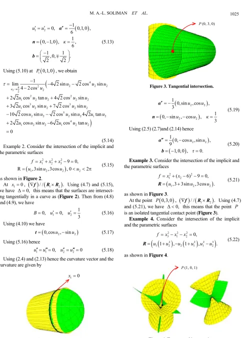
P (0, 3, 0)
Figure 3. Tangential intersection.
2 2
2 2
1
0,sin ,cos , 3
1 0, sin , cos ,
3
u u
u u κ
α
n
(5.19)
Using (2.5) (2.7)and (2.14) hence
2 2
1
0, cos ,sin , 9
1,0,0 , 0.
u u
τ
α
b
(5.20)
Example 3. Consider the intersection of the implicit and the parametric surfaces
2 2
1 2
1 2
( 6) 9 0, ,3 3sin ,3cos .
f x x
u u
R u2
(5.21)
as shown in Figure 3.
At the point P
0,3,0
,
f / / R1R2
. 0,Using (4.7) and (5.21), we have Δ this means that the point is an isolated tangential contact point (Figure 3).
P Example 4. Consider the intersection of the implicit and the parametric surfaces
2 2 2
3 1 2
2 2 2
1 2 2 1 1 2
0,
1 , 1 ,
f x x x
u u u u u u
R 3 . (5.22)
as shown in Figure 4.
[image:7.595.108.232.585.703.2]P (1, 0, 1)
At the point P
1,0,1
Sf SR,
on the intersection curve (Figure 4), we have
1 11 111
2 22 12
112 122 222
1 11 22 222
2 12 122 112
1,0, 2 , 0,0, 2 , 24,
0, 2,0 , 2,0,0 , 0, 2,0 , 0, 2,0 , 2,0,0 , 0,0, 6 ,
2, 10, 12,
0, 24, 0.
h
h h h h
h h h h
R R
R R R
R R R
(5.23) Using (3.8) and (5.23), we obtain
0,1,0 t (5.24) Using (3.12) (3.13) and (5.23) we obtain
2,0,3 ,
2 3
( ,0, ), 13
13 13 κ
α
n . (5.25) Using (2.5) (2.7) (2.14) (3.17) and (5.25) we obtain
3 3
, 19, ,
4 4
3 ,0, 2 , .
52
13 13 τ
α
b 3
(5.26)
6. Conclusions
Algorithms for computing the differential geometry prop-erties of intersection curves of implicit and parametric sur-faces in are given for transversal and tangential inter-section. This paper is an extension to the works of Ye and Maekawa [1]. They gave algorithms to compute the dif-ferential geometry properties of intersection curves be-tween two parametric surfaces then they applied it on a simple example for implicit and parametric surfaces inter-section. This paper presented direct and simple formulas to compute all differential geometry properties, which may reduce the time it takes to calculate those properties. The types of singularities on the intersection curve are charac-terized. The questions of how to exploit and extend these algorithms to compute the differential geometry properties of intersection curves between three surfaces in , can be topics of future research.
3
4
7. Acknowledgements
The authors would like to thank the reviewers for their
valuable comments and suggestions.
8. References
[1] X. Ye andT. Maekawa, “Differential Geometry of Inter-section Curves of Two Surfaces,” Computer-Aided Geo-metric Design, Vol. 16, No. 8, September 1999, pp. 767- 788. doi:10.1016/S0167-8396(99)00018-7
[2] C. L. Bajaj, C. M. Hoffmann, J. E. Hopcroft and R. E. Lynch, “Tracing Surface Intersections,” Computer-Aided Geometric Design, Vol. 5, No. 4, November 1988, pp. 285-307. doi:10.1016/0167-8396(88)90010-6
[3] N. M. Patrikalakis, “Surface-to-Surface Intersection,” IEEE Computer Graphics & Applications, Vol. 13, No. 1, January-February 1993, pp. 89-95.
doi:10.1109/38.180122
[4] T. J. Willmore, “An Introduction to Differential Geome-try,” Clarendon Press, Oxford, 1959.
[5] M. Düldül, “On the Intersection Curve of Three Paramet-ric Hypersurfaces,” Computer-Aided GeometParamet-ric Design, Vol. 27, No. 1, January 2010, pp. 118-127.
doi:10.1016/j.cagd.2009.10.002
[6] E. Kruppa, “Analytische und Konstruktive Differentialgeometrie,” Springer, Wien, 1957.
[7] E. Hartmann, “G2 Interpolation and Blending on Sur-faces,” The Visual Computer, Vol. 12, No. 4, 1996, pp. 181-192. doi: 10.1007/s003710050057
[8] G. A. Kriezis, N. M. Patrikalakis and F.-E. Wolter, “Topological and Differential Equation Methods for Sur-face Intersections,” Computer-Aided Geometric Design, Vol. 24, No. 1, January 1992, pp. 41-55.
doi:10.1016/0010-4485(92)90090-W
[9] R. C. Luo, Y. Ma and D. F. McAllister, “Tracing Tan-gential Surface-Surface Intersections,” Proceedings Third ACM Solid Modeling Symposium, Salt Lake City, 1995, pp. 255-262. doi:10.1145/218013.218070
[10] O. Aléssio, “Differential Geometry of Intersection Curves in 4 of three Implicit Surfaces,” Computer-Aided Geometric Design, Vol. 26, No. 4, May 2009, pp. 455- 471. doi:10.1016/j.cagd.2008.12.001
[11] M. P. do Carmo, “Differential Geometry of Curves and Surface,” Prentice Hall, Englewood Cliffs, NJ, 1976. [12] J. J. Stoker, “Differential Geometry,” Wiley, New York,
1969.