Accepted
Article
This article has been accepted for publication and undergone full peer review but has not
Methods in Ecology and Evolution
MR ERIC JOHN HOWE (Orcid ID : 0000-0002-4715-3958)
Article type : Research Article
editor: Professor Jason Matthiopoulos
Title: Model selection with overdispersed distance sampling data
Eric J Howe*, 1, 2, Stephen T Buckland1, Marie-Lyne Després-Einspenner3, Hjalmar S. Kühl3,
4
1
Centre for Research into Ecological and Environmental Modelling, University of St Andrews, The Observatory, Buchanan Gardens, St Andrews, Fife KY16 9LZ, UK
2
Wildlife Research and Monitoring Section, Ontario Ministry of Natural Resources and Forestry, DNA Building, Trent University, 2140 East Bank Drive, Peterborough, ON, K9L 1Z8, Canada
3
Max Planck Institute for Evolutionary Anthropology, Deutscher Platz 6, 04103, Leipzig, Germany
4
German Centre for Integrative Biodiversity Research (iDiv) Halle-Jena-Leipzig, Deutscher Platz 5e, 04103, Leipzig, Germany
Accepted
Article
Abstract
1. Distance sampling (DS) is a widely-used framework for estimating animal abundance. DS models assume that observations of distances to animals are independent. Non-independent
observations introduce overdispersion, causing model selection criteria such as AIC or AICc
to favour overly complex models, with adverse effects on accuracy and precision. 2. We describe, and evaluate via simulation and with real data, estimators of an
overdispersion factor ( ̂), and associated adjusted model selection criteria (QAIC) for use
with overdispersed DS data. In other contexts, a single value of ̂ is calculated from the
“global” model, i.e., the most highly-parameterized model in the candidate set, and used to
calculate QAIC for all models in the set; the resulting QAIC values, and associated ΔQAIC
values and QAIC weights, are comparable across the entire set. Candidate models of the DS detection function include models with different general forms (e.g., half-normal, hazard rate, uniform), so it may not be possible to identify a single global model. We therefore propose a two-step model selection procedure by which QAIC is used to select among models with the same general form, and then a goodness-of-fit statistic is used to select among models with different forms. A drawback of this approach is that QAIC values are not comparable across all models in the candidate set.
Accepted
Article
4. Many DS surveys yield overdispersed data, including cue counting surveys of songbirds and cetaceans, surveys of social species including primates, and camera-trapping surveys. Methods that adjust for overdispersion during the model selection stage of DS analyses therefore address a conspicuous gap in the DS analytical framework as applied to species of conservation concern.
Keywords: animal abundance, camera trapping, cue counting, distance sampling, model selection, overdispersion, QAIC
Introduction
Distance sampling (DS) is an established framework for estimating animal abundance (Buckland et al. 2001, 2004; Borchers, Buckland & Zucchini et al. 2002). It allows for imperfect detection by assuming detection probability is a function of the distance between objects (e.g., animals or their sign), and observers. Careful modelling of this function is required to obtain accurate abundance estimates (Buckland et al. 2001, 2004). Exploratory analyses, goodness-of-fit (GOF) testing, and model selection are therefore critical
Accepted
Article
both distance sampling, and information-theoretic model selection, as described by Buckland et al. (2001, 2004), and Burnham and Anderson (2002).
DS methods assume that observations are independent (Buckland et al. 2001), but some DS surveys violate this assumption. For example, some animals travel in groups. Violation of the independence assumption can be avoided by treating the group as the unit of observation, measuring or estimating distances to the center of detected groups, and
estimating animal density as the product of group density and mean group size (Buckland et al. 2001). However, this is only effective if the size and central location of the group are measured accurately (Buckland et al. 2001, 2010). When they cannot be, for example because groups are widely-spread or in motion, the recourse is to treat the individual as the unit of observation, and to record distances to all group members detected, in which case the data include non-independent observations. Furthermore, some animals, such as cetaceans that are often submerged, or songbirds that perch concealed in trees, are only available to be observed intermittently. However, if they give discrete cues of their presence and location, such as whale blows or bursts of birdsong, density of cues can be estimated using DS
Accepted
Article
the independence assumption do not bias point estimates of model parameters, but introduce overdispersion (Buckland et al. 2001).
When distance data are overdispersed: (1) GOF tests, and likelihood ratio tests (LRTs) to compare the fit of nested models, are invalid and prone to reject the null hypotheses that a model adequately fits the data (GOF tests), or that the simpler of two models provides a better fit than a more complex one (LRTs); (2) model-based analytic variances underestimate the actual uncertainty associated with the estimates, though
empirical design-based estimators are robust (Fewster et al. 2009), and bootstrap estimators that resample points or transects are unaffected (Buckland 1984); (3) model selection criteria that have not been adjusted for overdispersion favour overly complex models with more than the optimal number of parameters (Cox and Snell 1989; Burnham and Anderson 2002; Buckland et al. 2001, 2010). Akaike’s Information Criterion (AIC; Akaike 1973) is usually recommended for selecting among candidate models of the detection function (Buckland et al. 2004; Marques et al. 2007), however, if the data are overdispersed, AIC is likely to favour unnecessarily complex models (Buckland et al. 2001, 2010; Buckland 2006). This additional complexity reduces precision, and can cause bias if it affects the slope of the detection function near the point. Criteria adjusted to account for overdispersion have not been developed previously.
Accepted
Article
estimated from a common detection function (Buckland et al. 2004; Marques et al. 2007). Observations within different strata can be analyzed separately to avoid this bias, but this can reduce sample sizes to the point where densities of some strata may not be estimable, or estimates may be too imprecise to be useful. The multiple covariate approach to DS analysis improves efficiency by modelling variation in detectability using covariates (Buckland et al. 2004; Marques et al. 2007). It also casts decisions about how much stratification is necessary as a model selection problem, but in this case the quality of inferences about strata-specific densities is affected by the reliability of the model selection criterion. When the
independence assumption is suspected or known to have been violated, it has been
recommended that analysts constrain the complexity of the detection function and the number of covariates to avoid overfitting (Buckland et al. 2004, 2010; Marques et al. 2007).
However, limiting the candidate set to simple models may not be desirable if there are multiple potential covariates of the detection function. Model selection criteria unadjusted for overdispersion will tend to select models that subdivide the data more than necessary, with adverse effects on precision. Conversely, “underfitting”, i.e., failure to include significant sources of variation in the estimating model, would cause stratum-specific densities to be underestimated if true detection probabilities in that stratum tend to be lower, and vice versa. Adjusted criteria could underfit if they overcompensated for overdispersion (e.g., if the magnitude of overdispersion was overestimated).
Although explicitly modeling the sources of overdispersion would be ideal, this is not always possible or practical with real data (Cox and Snell 1989; Lebreton 1992; Burnham and Anderson 2002). An approximation that is often sufficient in practice is to estimate a single,
omnibus overdispersion factor ( ̂) from a χ2 GOF test of the global model (i.e., the most
highly parameterized or most general model) divided by its degrees of freedom (df), and to
Accepted
Article
in the candidate set (Cox and Snell 1989; Lebreton 1992; Liang and McCullagh 1993; Burham and Anderson 2001, 2002). The adjusted version of AIC (QAIC) is:
= −2 log
̂ + 2
where log L is the log likelihood value, is a vector of maximum likelihood parameter
estimates, and K is the number of parameters in the current model (Lebreton et al. 1992).
Burnham and Anderson (2001, 2002) clarified that ̂ should be included as one of the K
parameters.
Given an estimator of c ( ̂), the same approach could be used to calculate QAIC for
models of the DS detection function. However, candidate sets usually include models with different general forms (termed “key functions”; e.g., half-normal, hazard rate, and uniform; Buckland et al. 2001) as well as different numbers of adjustment terms and covariate
combinations (Buckland et al. 2004; Marques et al. 2007). Models with different key
functions are not nested, hence it may not always be straightforward to identify a single
“global” model from which to estimate ̂. Below we propose and evaluate two estimators of
̂, and a two-step model selection procedure that does not require that a single global model is
identifiable, for use with overdispersed DS data.
Methods
Model selection criteria and procedures
We suggest the χ2 GOF statistic for binned distance data (Buckland et al. 2001, p. 71,
eqn. 3.57) divided by its degrees of freedom as one estimator of c ( ̂1). To allow for the
Accepted
Article
each key function, and in step two we compare the GOF of the best-supported models with
different key functions. More specifically, in step one, we obtain ̂ from the most
parameterized model within each key function (rather than from the most
highly-parameterized model overall), use those values of ̂ to calculate QAIC for all models with
the same key function, and use QAIC to identify the best-supported model within each key
function. In this step, the same value of ̂ is used to calculate QAIC for all models with the
same key function, but different values of ̂ are used to calculate QAIC for different key
functions. In step two, we compare values of the χ2 GOF statistic divided by its df across
QAIC-selected models (one from each key function), and choose the model with the smallest value for estimation. If continuous distances are recorded in the field, distance observations will first need to be grouped into categories so that the GOF test for binned data can be performed. See Buckland et al. (2001) for advice regarding binning continuous observations.
The number of distance observations recorded per independent encounter between an animal and an observer provides an alternative measure of the magnitude of overdispersion
( ̂ ). ̂ will often be calculable from the raw data, and will be the same for all models in the
candidate set. In CT surveys of solitary animals, ̂ would be the mean number of distance
observations recorded during a single pass by an animal in front of a CT. In surveys of social
animals employing human observers, ̂ would be the mean number of detected animals per
detected group, and in CT surveys of social animals ̂ would be the mean number of
distance observations recorded during an encounter between a group of animals and a CT. ̂
could be used instead of multiple values of ̂ to calculate QAIC values as in step one above.
QAIC values would still be compared only within key functions, and the χ2 GOF statistic
divided by its df would still be used in step two to select among QAIC-selected models with
different key functions. Hereafter, we will refer to QAIC calculated from ̂ as QAIC1, and
Accepted
Article
Simulations
We conducted simulations where non-independent observations were all at the same distance so that we could evaluate performance where the true magnitude of overdispersion
(c), and the true underlying model were known, but we would not expect this scenario to arise
in practice. When non-independent observations during a single independent encounter are at different distances (e.g., to different members of a group, different cues from a moving
animal, or as an animal moves past a CT), true c is unknown because the different distance
observations contribute information about the shape of the detection function. We therefore also simulated camera-trapping (CT) surveys of moving animals where cameras recorded video and distance was recorded every two seconds as animals moved through the field of
view. These simulations mimic real surveys where animals move and c is unknown.
Furthermore, the distribution of observed distances differed from the expected distribution of independent detections (see Supplemental Material), so the true underlying model was also unknown.
For the simulations with known c, we sampled distances to animals within a circular
point transect with radius 20 m, where the true density was 2.00 / m2. To generate
independent DS data, we simulated detections via random trials where detection probability
declined according to a half-normal function with scale parameter (σ) of 7. Each observation
was arbitrarily assigned one of three levels of a spurious categorical covariate that had no effect on detectability, which we will refer to as “observer”. We then replicated each data set
5 times to generate overdispersed data with c = 6. We fitted eight point transect DS models
Accepted
Article
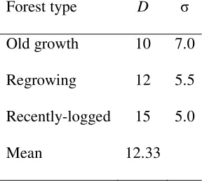
For the CT surveys, we simulated sampling of ungulates inhabiting old growth forests, recently-logged forests, and previously logged but regrowing forests. Simulation parameters were based on Howe et al.’s (2017) survey of Maxwell’s duikers, but were also selected to ensure that data were overdispersed, not sparse, and included multiple potential covariates of detectability. We assumed that the density of understory vegetation increased immediately after logging and decreased gradually as forests regrew, such that food supply and therefore animal density was highest, but detection probability as a function of distance was lowest, in recently-logged forests; we further assumed a larger difference in detection probability between old growth and logged forests than between recently-logged and regrowing forests (Table 1).
We simulated movements of 10, 12, and 15 animals within 1 km2 study areas in old
growth, regrowing, and recently-logged habitats, respectively. Each animal started with a random initial location and heading, after which new locations were generated every two seconds for 12 hours. Step lengths were drawn from an exponential distribution with a rate parameter of 2, and turn angles were drawn from a normal distribution with mean of 0 and standard deviation of 0.05 radians. Animals that moved beyond the boundaries of the study areas reappeared on the opposite side of the same study area at the same heading. We simulated sampling at a grid of 36 CTs at 150 m spacing within each study area. We defined the zone of potential detection by a CT as a sector with a central angle of 0.733 radians and a radius of 25 m, and recorded distances between CTs and animal locations that fell within these sectors. We initially conducted random trials according to a half-normal function with
σ as in Table 1 to determine whether animals were detected at each time step. However, we
Accepted
Article
sector defined by the location and angle of view of the CT, at predetermined snapshot moments after initial detection, following Howe et al. (2017). Each animal travelled 10.7 to 11.0 km in a meandering path over 12 hours. Most step lengths were between 0 and 0.5 m, which ensured that animals would be observed multiple times, including at similar distances, during each independent encounter, and hence distance data would be severely overdispersed. Density remained constant, and the expected distribution of animal locations was uniform within each study area.
We analysed data from all three habitat types simultaneously using multiple covariate distance sampling. Different habitat types were treated as different strata, with the potential to estimate a common detection function across all strata, or to model differences in
detectability among strata using categorical covariates affecting the scale parameter of the detection function. We considered a habitat type covariate with two levels (old growth or logged), and one with three levels (old growth, regrowing, and recently-logged). The 36 cameras in each study area were arbitrarily assigned to one of three different CT models (12 of each type). Detectability therefore varied among habitat types (Table 1) but not among camera trap models. Both habitat type and camera trap model were considered as potential covariates of the detection function; only one habitat type covariate was included in any model. We fitted twenty models with either the half-normal or hazard rate key function, 0 or 1 cosine adjustment terms, and different covariate combinations to each data set.
During both sets of simulations, distance data were binned into intervals prior to analysis. Howe et al. (2017), were confident of their assignments of duikers into 1 m
Accepted
Article
estimated parameters, the log-likelihood value, the estimated density ( ) and associated
empirical, design-based variances (Fewster et al. 2009), and the χ2 GOF statistic and its df
and P-value, from all models fit to each data set. We selected among candidate models by
comparing AIC values across all models fitted to the same data set, and using both QAIC1
and QAIC2 following the two-step procedure described in the methods section. Simulations
were performed using R software, version 3.3.2 (R Core Team 2016).
Applications with real data
We applied the same model selection criteria and procedures used in the simulations to real data from Maxwell’s duikers in Taï National Park, Côte d’Ivoire, originally presented in Howe et al. (2017). We also reanalyzed point count data from singing males of four species of songbirds sampled at Montrave Estate in Fife, Scotland, originally presented in Buckland (2006). The Montrave study area was small enough that densities of singing males were estimable by mapping their territories; these estimates were expected to have low bias, and served as benchmarks by which the accuracy of DS estimates were assessed (Buckland 2006). Aware of the potential for overdispersion and therefore overfitting with cue count data, Buckland (2006) did not consider models with >2 parameters, and used a combination of AIC and plots of fitted probability density functions and detection functions to select among six models with different key functions and numbers of adjustment terms. We fitted a total of 9 models to each data set (uniform with 1, 2, or 3 cosine adjustment terms, half-normal with 0, 1, or 2 Hermite polynomial adjustment terms, and hazard rate with 0, 1, or 2
cosine adjustment terms) and used the two-step procedure with QAIC1 to select among them.
Truncation distances and cutpoints for the χ2 GOF test followed Buckland (2006). QAIC2
Accepted
Article
and exclude implausible models, such as cases where estimated detection probabilities exceeded 1.0, or fitted detection functions that were not monotonically nonincreasing.
Results
Simulations
In simulations where c and the correct underlying model were known, mean sample
sizes of distance observations in overdispersed data sets was 3630. The χ2 GOF test rejected
the null hypothesis of adequate fit of the correct model for 492 of 500 data sets. ̂ varied
among iterations, but on average it estimated the true magnitude of overdispersion reasonably
accurately (mean and median ̂ from the data generating model were 6.16 and 5.73,
respectively; true c was 6.0). AIC selected the most highly-parameterized model most
frequently, selected models with the spurious observer covariate for 71.4% of data sets, and selected the correct model for only 2.8% of data sets (Table 2). QAIC selected the correct model most frequently, followed by the hazard rate model with one adjustment and no
covariates. QAIC1 and QAIC2 selected models with the spurious covariate for 14% and 13%
of data sets, respectively (Table 2). from QAIC-selected models was both more accurate and more precise than from AIC-selected models (Table 3).
Accepted
Article
from the CT continued to contribute observations at longer distances where detection probability would otherwise be low. As a result, hazard rate models frequently provided a better fit than the half-normal model from which the random detections were simulated (Fig. S1).
The χ2 GOF test rejected the null hypothesis of adequate fit of 89% of the 10000
models fitted. Sample sizes, and numbers of observations per independent encounter ( ̂ ),
were slightly higher in old growth forests where detection probability as a function of
distance was highest, even though densities there were lowest (Table 4). ̂ was generally
lower, indicating less overdispersion, than ̂ from a given data set and model; ̂ was also
more variable among iterations than ̂ (Table 4).
AIC again tended to select highly-parameterized models. Density was not estimable from the AIC-minimizing model in 9 cases, and in 53 other cases, estimates were
unrealistically high (>10 times the true density). QAIC1 and QAIC2 each selected models
from which density was not estimable twice, and from which density was severely overestimated 4 times; these problems were associated with the same six data sets. AIC favoured detection function models with more complex forms, selecting adjusted hazard rate models for 49% of data sets, and either unadjusted hazard rate or adjusted half normal models for another 45%, whereas QAIC selected unadjusted hazard rate models most frequently, followed by unadjusted half normal models (Table 5). AIC always supported an effect of habitat type on detection probability, and supported the 3-level habitat covariate for 77% of
data sets (Table 5). QAIC1 and QAIC2 selected models with habitat type covariates for 89%
and 81% of data sets, respectively, but tended to favour the 2-level covariate (selected for 59% and 68% of data sets, respectively) over the 3-level covariate (Table 5). Most (88% of)
AIC-selected models, 27% of QAIC1-selected models, and 5% of QAIC2-selected models
Accepted
Article
iterations was greatest with QAIC1 (Table 5), which is not surprising given the variability of
̂ across data sets (Table 4).
QAIC2 and the two-step model selection procedure maximized both the accuracy and
precision of (Fig. 1, Table S1). AIC-selected models yielded negatively biased on average (Fig 1). AIC-selected models yielded the most accurate only in recently-logged forests (Fig. 1). QAIC-selected models rarely included the 3-level habitat covariate, and as a result, in recently-logged forests, and differences in among habitat types, were
underestimated (Fig 1, Table S1). However, QAIC-selected models yielded more accurate estimates of total density, and of density in regrowing and old growth forests (Fig. 1).
QAIC2-selected models yielded the most precise density estimates, followed by QAIC1
-selected models (Table S1).
Applications with real data
The number of observations of Maxwell’s duikers per independent encounter ( ̂ ) was
15.35 during the daytime, and 16.98 during times of peak activity. The χ2 GOF statistic
divided by its df ( ̂ ) from different models fitted to the daytime data set ranged between 20
and 25, and from models fitted to the peak activity data set ranged between 12 and 35 (Tables S2 & S4). Model selection criteria and procedures adjusted for overdispersion selected the same models as AIC for estimation from each data set (the unadjusted hazard rate model, see Howe et al. 2017 and Tables S2–S5), so was unaffected.
In our reanalysis of songbird data from Montrave Estate, QAIC1 did not consistently
outperform either AIC, or the combination of AIC, a constrained candidate model set, and
reference to diagnostic plots employed by Buckland (2006). Model selection via QAIC1
Accepted
Article
1). See the supplemental material for a detailed description of the results of our reanalysis including comparisons to models selected by AIC and Buckland (2006).
Discussion
Simulations with known c demonstrated that: (1) AIC was prone to overfitting,
selecting unnecessarily complex models, (2) ̂ was an accurate if variable estimator of the
true magnitude of overdispersion, and (3) QAIC and our two-step procedure outperformed AIC in that it selected the correct underlying model more frequently, and QAIC-selected models yielded more accurate and precise than AIC-selected models.
Our simulations with animal movement were designed to be challenging from a model selection perspective, in that we sought criteria and procedures that would support small but real differences in detectability while excluding spurious effects from estimating models. AIC consistently supported models with adjustment terms even though density was sometimes inestimable or drastically overestimated by these models, and models with a covariate that had no real effect on detectability. Associated inferences regarding both animal abundance and sources of variation in detectability were flawed. Models selected by QAIC and our two-step model selection procedure included fewer adjustment terms, were much less likely to include the spurious CT model covariate, and yielded more accurate and precise . Of the two proposed estimators of the magnitude of overdispersion, the mean
number of observations per independent encounter ( ̂ ) was more consistent than the χ2 GOF
statistic divided by its degrees of freedom ( ̂1). QAIC2-selected models yielded the most
accurate and precise density estimates on average.
Accepted
Article
the optimal model. This may not indicate that QAIC will underfit generally because the difference in detectability between recently-logged and regrowing forests was slight. Furthermore, the effect of certain detection after initial detection on the distribution of observed distances would have obscured differences between study areas. Sources of variation in detectability that have small effect sizes may go undetected by any model selection criteria. Nevertheless, failure to detect and support this difference in our simulated data caused underestimation of density where detection probability was lowest. The
difference in density between recently-logged and other forest types was therefore underestimated, however, differences among all three habitat types were still apparent.
We applied model selection criteria and procedures “blindly”, in that we always
estimated from the model that minimized AIC, or χ2 / df from the QAIC-minimizing model
within each key function. AIC might have performed better if we had followed established practices for DS analyses and multimodel inference, including exploratory analyses of relationships between distance observations and covariates, careful examination of fitted
detection functions and associated parameter estimates, and consideration of ΔAIC values
and AIC weights (Buckland et al. 2001, 2004; Burnham and Anderson 2002; Marques et al. 2007). Therefore our results, where adjusting for overdispersion improved inferences from simulated data, but only improved inferences from real data in one of six cases, as well as Buckland et al.’s (2010) simulation results, suggest that adverse effects of overfitting by AIC may often be minor. Furthermore, our two-step approach to model selection using QAIC leads to the selection of a single model for estimation. QAIC values are not comparable
between key functions, so metrics like ΔQAIC and QAIC weights cannot be used to compare
Accepted
Article
We did not attempt to fit density surface models that allow researchers to assess support for covariation between density and spatially referenced covariates (Hedley and Buckland 2004; Miller et al. 2013). However, we note that such analyses can be performed either in two stages, where detectability is estimated during the first stage, and plot-specific counts or abundance estimates are modelled during the second stage, or by maximizing a full likelihood model whereby parameters related to both detectability and local abundance are estimated simultaneously (Hedley and Buckland 2004; Johnson, Laake & Ver Hoef 2010; Miller et al. 2013). If a two-stage approach to fitting density surface models is adopted, any model selection criteria or procedures, including those described here, could be used when estimating detectability. It is therefore possible to account for overdispersion in the distance data when estimating the detection function, and still fit density surface models to test for effects of spatial covariates on density. Johnson, Laake & Ver Hoef (2010) proposed a one-stage, model-based approach for simultaneously estimating detectability and spatially
variable abundance from DS data. They also evaluated the effectiveness of an overdispersion
factor calculated from a χ2 test performed on transect-specific counts for inflating
model-based variances around abundance estimates to account for overdispersion introduced by fine-scale variation in local abundance. They found that variances were still underestimated
except where there were many transects, and suggested the χ2 GOF test for binned distance
data divided by its degrees of freedom (our ̂ ) as an alternative estimator. However, it is not
clear to us how a statistic derived from the observed distances would quantify overdispersion induced by variation in local abundance, and we prefer to use this statistic to adjust for overdispersion only when modeling the detection function.
Accepted
Article
et al. (2010) simulated line transect sampling of primate groups and found that treating the individual as the unit of observation and selecting among models of the detection function using AIC yielded more accurate and precise than approaches that treated the group as the unit of observation, “despite obvious overfitting in some cases” (p. 835).
Synthesis and recommendations
We described novel approaches to estimating an overdispersion factor ( ̂), and
QAIC-based procedures for selecting among models of the DS detection function when the assumption that observations are independent is violated. These novel methods improved inference from simulated data. However, we conducted limited simulations with severely overdispersed data, and reanalyses of real data sets did not unambiguously indicate that adjusting for overdispersion at the model selection stage improved inference. We therefore recommend additional research, but also that these criteria and procedures be considered as alternatives to AIC when the independence assumption is violated. They are most likely to be useful where: (1) overfitting by AIC is apparent (e.g., if AIC favours models that include both adjustment terms and covariates, multiple adjustment terms, or weak or imprecisely-estimated covariate effects); (2) it is not practical or not desirable to constrain the candidate set to include only simple models (e.g., where there are multiple potential covariates of the detection function, or where models with unadjusted key functions do not fit the observed data well); or (3) where researchers wish to avoid subjectivity during model selection.
Acknowledgements
Accepted
Article
permission to conduct field research in Taï National Park, Dr. Roman Wittig for permitting data collection in the area of the Taï Chimpanzee Project, and Dr. Joeseph Nocera for informal discussions about model selection in the presence of overdispersion.
Data Accessibility
Data from Maxwell's duikers in Tai National Park are archived at the Dryad data repository (https://doi.org/10.5061/dryad.b4c70) (Howe et al. 2017), as are the raw Montrave Estate cue count data (https://doi:10.5061/dryad.j2p2h3s), which are also available as Distance projects at https://synergy.st-andrews.ac.uk/ds-manda/#montrave-songbird-case-study and
http://distancesampling.org/.
Authors’ contributions
EJH and STB conceived the ideas, EJH analysed the data and led the writing of the
manuscript. M.-L.D.-E. helped to design and conducted the field study of Maxwell’s duikers, H.S.K. designed the field study of Maxwell’s duikers. All authors contributed critically to the drafts and gave final approval for publication.
Literature Cited
Akaike H. 1973. Information Theory as an Extension of the Maximum Likelihood Principle.
Pp. 267-281 in BN Petrov and F Csaki (eds.) Second International Symposium on
Information Theory. Akademiai Kiado, Budapest, Hungary
Borchers DL, Buckland ST, Zucchini W. 2002. Estimating animal abundance: closed populations. Springer Science & Business Media, New York, USA
Accepted
Article
Buckland ST. 2006. Point transect surveys for songbirds: robust methodologies. The Auk 123:345–357
Buckland ST, Anderson DR, Burnham KP, Laake JL, Borchers DL, Thomas L. 2001. Introduction to distance sampling: estimating abundance of biological populations. Oxford University Press, Oxford, UK
Buckland ST, Anderson DR, Burnham KP, Laake JL, Borchers DL, Thomas L. 2004. Advanced distance sampling: estimating abundance of biological populations. Oxford University Press, Oxford, UK
Buckland ST, Plumptre AJ, Thomas L, Rexstad EA. 2010. Design and analysis of line transect surveys for primates. International Journal of Primatology 31:833–47
Burnham KP, Anderson DR. 2001. Kullback-Leibler information as a basis for strong inference in ecological studies. Wildlife research 28:111–119
Burnham KP, Anderson DR. 2002. Model selection and inference: a practical information theoretic approach. Second edition. Springer Science and Business Media, New York, USA Cox DR, Snell EJ. 1989. Analysis of binary data. Second edition. Chapman and Hall, New York, USA
Fewster RM, Buckland ST, Burnham KP, Borchers DL, Jupp PE, Laake JL, Thomas L. 2009. Estimating the encounter rate variance in distance sampling. Biometrics 65:225–236
Hedley SL, Buckland ST. 2004. Spatial models for line transect sampling. Journal of Agricultural, Biological, and Environmental Statistics 9:181–199
Howe EJ, Buckland ST, Després‐Einspenner ML, Kühl HS. 2017. Distance sampling with
camera traps. Methods in Ecology and Evolution 8:1558–1565
Johnson DS, Laake JL, Ver Hoef JM. 2010. A model‐based approach for making ecological
Accepted
Article
Johnson JB, Omland KS. 2004. Model selection in ecology and evolution. Trends in ecology & evolution 19:101–108
Lebreton J-D, Burnham KP, Clobert J, Anderson DR 1992. Modeling survival and testing biological hypotheses using marked animals: a unified approach with case studies. Ecological Monogrographs 62:67–118
Liang K-Y, McCullah P. 1993. Case studies in binary dispersion. Biometrics 49:623–630 Marques TA, Thomas L, Fancy SG, Buckland ST. 2007. Improving estimates of bird density using multiple-covariate distance sampling. The Auk 124:1229–1243
[image:22.612.235.379.460.589.2]Miller DL, Burt ML, Rextad EA, Thomas L. 2013. Spatial models for distance sampling data: recent developments and future directions. Methods in Ecology and Evolution 4:1001–1010 R Core Team. 2016. R: A language and environment for statistical computing. R Foundation for Statistical Computing, Vienna, Austria. URL https://www.R-project.org/
Table 1. Animal densities (D) and scale parameters (σ) of a half normal detection probability
function in different habitat types used to generate simulated distance sampling data.
Forest type D σ
Old growth 10 7.0
Regrowing 12 5.5
Recently-logged 15 5.0
Accepted
[image:23.612.155.461.197.461.2]Article
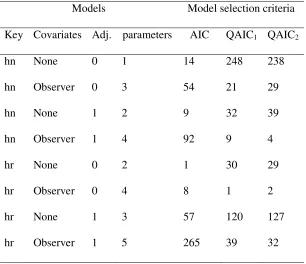
Table 2. Number of times each detection function model fitted to simulated, overdispersed
data from stationary animals was selected by AIC, and by each of QAIC1 and QAIC2
following the two-step procedure described in the methods section, of 500 replicate iterations. “Key” denotes the key function, either half-normal (hn) or hazard rate (hr); “Adj.” denotes the number of adjustment terms.
Models Model selection criteria
Key Covariates Adj. parameters AIC QAIC1 QAIC2
hn None 0 1 14 248 238
hn Observer 0 3 54 21 29
hn None 1 2 9 32 39
hn Observer 1 4 92 9 4
hr None 0 2 1 30 29
hr Observer 0 4 8 1 2
hr None 1 3 57 120 127
Accepted
[image:24.612.207.407.171.257.2]Article
Table 3. Medians of density estimates ( ) and of coefficients of variation (CV) of those estimates, from models fitted to simulated, overdispersed data from stationary animals,
selected by AIC, and by QAIC1 and QAIC2 following the two-step procedure, across 500
iterations. True D was 2.00.
AIC QAIC1 QAIC2
Median 1.89 2.00 2.00
Median CV ( ) 0.054 0.029 0.028
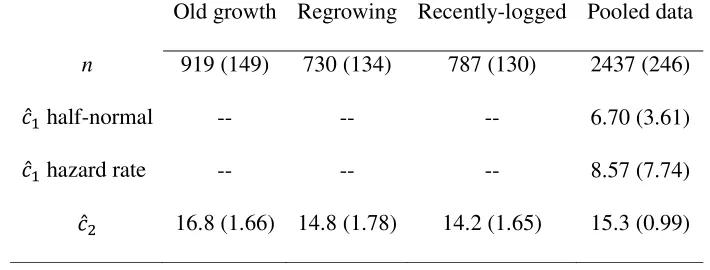
Table 4. Mean (SD) sample sizes (n) of distance observations and numbers of observations
per independent encounter ( ̂ ) from each habitat type and from data pooled across habitat
types, and mean values of the χ2 GOF statistic divided by its degrees of freedom ( ̂ ) from the
most highly parameterized half-normal and hazard rate models fitted to the pooled data sets, across 500 iterations.
Old growth Regrowing Recently-logged Pooled data
n 919 (149) 730 (134) 787 (130) 2437 (246)
̂ half-normal -- -- -- 6.70 (3.61)
̂ hazard rate -- -- -- 8.57 (7.74)
[image:24.612.128.483.413.548.2]Accepted
[image:25.612.139.471.249.714.2]Article
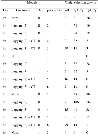
Table 5. The number of times, out of 500 iterations, that each of the 20 candidate models was selected by each model selection criterion, and below this, the number of times each of four forms of the detection function, and each of three covariate effects, was included in the selected models. “Key” denotes the key function, either half-normal (hn) or hazard rate (hr); covariates were: Logging (2), with differences in detectability between logged and old growth forests, Logging (3), with differences among all habitat types, and camera trap model (CT), which did not affect detectability; “Adj.” denotes the number of adjustment terms.
Models Model selection criteria
Key Covariates Adj. parameters AIC QAIC1 QAIC2
hn None 0 1 0 8 26
hn Logging (2) 0 2 0 52 104
hn Logging (3) 0 3 3 34 19
hn Logging (2) + CT 0 4 9 32 7
hn Logging (3) + CT 0 5 20 14 3
hn None 1 2 0 0 0
hn Logging (2) 1 3 3 37 28
hn Logging (3) 1 4 6 22 5
hn Logging (2) + CT 1 5 16 18 0
hn Logging (3) + CT 1 6 71 13 0
hr None 0 2 0 45 70
hr Logging (2) 0 3 2 106 182
hr Logging (3) 0 4 15 48 35
hr Logging (2) + CT 0 5 31 31 12
hr Logging (3) + CT 0 6 79 18 1
Accepted
Article
hr Logging (2) 1 4 4 11 8
hr Logging (3) 1 5 28 2 0
hr Logging (2) + CT 1 6 50 7 0
hr Logging (3) + CT 1 7 163 2 0
Forms AIC QAIC1 QAIC2
hn (0 adjustment terms) 32 140 159
hn (1 adjustment term) 96 90 33
hr (0 adjustment terms) 127 248 300
hr (1 adjustment term) 245 22 8
Covariate effects AIC QAIC1 QAIC2
Logging (2-level) 115 294 341
Logging (3-level) 385 153 63
[image:26.612.140.473.63.405.2]CT model 439 135 23
Figure 1. Animal densities (on y-axes) estimated from AIC-, QAIC1- and QAIC2-selected
models fitted to simulated distance sampling data collected at camera traps in three different habitat types, and total density across all 3 habitat types. Dashed grey lines show true densities. Heavy black lines show medians across 438 and 494 AIC- and QAIC-selected models, respectively, from which density was estimable and the estimate of total density was within an order of magnitude of the true value. Whiskers extend 1.5 times the interquartile range from the boxes; outliers were excluded from the plots.
Figure 2. Densities of songbirds at Montrave Estate (on y-axes), estimated from models selected by Buckland (2006; “B2006” on x-axes), AIC-minimizing models, and models
selected by QAIC1. Densities estimated by mapping territories, which were assumed to have