Self stabilising target counting in wireless sensor networks using Euler integration

(1)

Self-stabilising target counting in wireless sensor

networks using Euler integration

Danilo Pianini

Universit`a di Bologna Cesena IT

[email protected]

Simon Dobson

University of St Andrews Scotland UK

[email protected]

Mirko Viroli

Universit`a di Bologna Cesena IT

[email protected]

Abstract—Target counting is an established challenge for sensor networks: given a set of sensors that can count (but not identify) targets, how many targets are there? The problem is complicated because of the need to disambiguate duplicate observations of the same target by different sensors. A number of approaches have been proposed in the literature, and in this paper we take an existing technique based on Euler integration and develop a fully-distributed, self-stabilising solution. We derive our algorithm within the field calculus from the centralised presentation of the underlying integration technique, and analyse the precision of the counting through simulation of several network configurations.

I. INTRODUCTION

Many sensor network problems can be expressed as an integration – in some sense – of locally-determined values. An obvious example is determining the average temperature of a room from point observations made by a field of sensors. Distributed and self-stabilising imple-mentations of such local-to-global calculations therefore provide a solid basis for addressing real-world sensing problems. However, the situation also gives rise to other questions such as: how good is the sampling that the sen-sor network makes of the phenomenon being observed?, what is the potential for missing key features not readily observable in the data?, and, how do observations from different sensors in a local area interact with one an-other? Robust sensing requires that we can both answer these questions in the abstract, and then propagate the answers throughout the distributed implementation.

In this paper we take a first step towards addressing these issues. We take an established challenge in sensor networks – detecting and estimating the number of targets in an area without being able to assign each individual target an identity – and an existing solution that uses concepts from algebraic topology, the Eu-ler integration technique proposed by Baryshnikov and

Ghrist [1], [2]. We develop a scalable, self-stabilising algorithm for computing an estimate of the number of targets, using the self-stabilising field calculus [3]. We show that the topological ideas map very naturally to field calculus structures in a way that is robust to some sorts of perturbations in sensors and targets, but that is also (it turns out) very sensitive to interactions between them. We believe that this work shows that field calculus is an appropriate basis for a class of algorithms that have a formal semantic basis in algebraic topology, which suggests in turn that such algorithms may form a useful approach to a range of problems in distributed and per-vasive systems. We use our implementation to stress the algorithm under diverse conditions in terms of sensors displacement, sensing capabilities, and target counting. In doing so, we identify both strong and weak points of the technique, and develop some recommendations for those wanting to use or extend it.

Our paper makes two contributions: to show that the field calculus can be used to implement algorithms requiring a significant amount of algebraic topology; and to explore the relationships between sensor density, target density, and estimation accuracy. The former is interesting in extending the reach of field calculus, and of self-organisation techniques in general; the latter is a starting point for a more rigorous approach to the study of the quality of sensor-derived information.

(2)

II. BACKGROUND

A. Target counting

The target counting problem can be stated succinctly as follows: Suppose we have a sensor that can detect the presence of targets within a certain region. An example would be a sensor that detects short-range “chirps” from badges worn by individuals. The sensor cannot identify

individual targets, it can only count the number it can see. Put several of these sensors into a space together with several (stationary) targets, and collect their counts: How many targets are there? The subtlety of the problem arises because severaldifferentsensors may be observing the same target, and so we need a way to eliminate duplicate observations.

This problem has received extensive treatment in the literature: see Wu at alia [4] for a recent survey and comparative evaluation (which does not however cover the technique we use here). Most approaches make use of detailed knowledge (or assumptions) about the sensor coverage, typically using geometric constraints: for ex-ample Gandhiet alia[5] require minimal overlaps in the coverage. Statistical approaches are also possible: Guoet alia[6] again use geometry to develop a probability mass function over the space of co-observation. The problem is closely related to the coverage problem of estimating (or ensuring) that a set of sensors cover an area.

B. Field calculus

The algorithms discussed in this paper can be im-plemented on top of a variety of distributed models of computation, as its basic assumption is that de-vices communicate local information asynchronously with neighbours. However, in presenting design and technical details we shall use the field calculus compu-tational model [7], [3] and its incarnation in the Protelis language [8]. They are at the core of the aggregate com-puting paradigm [9], recently proposed as an approach for designing resilient distributed systems by abstracting away from individual devices behaviour and focusing on the global, aggregate behaviour of the collection of devices. This approach provides smooth composition of distributed behaviour, allowing the development of highly reusable “building block” operators, a candidate of which is the target counting solution considered in this paper.

The unifying abstraction of field calculus is a model of the distributed data structures that can be collectively manipulated as a “computational field” (or “field” for short), inspired by physical concepts like magnetic fields,

that maps each device in a network to a local value of some sort. In field calculus every expression, value or variable is a field: for example, a collection of temper-ature sensors produce a field of ambient tempertemper-atures, smart-phone accelerometers produce a field of movement directions, a notification application produces a field of messages currently being displayed on those phones, and a field of vectors might guide the movement of autonomous drones.

Such fields are constructed and manipulated using four syntactic program constructs:

• Functions: f(e1,...,en) applies function f to

arguments e1,...,en. The function can be a

“built-in” primitive (any stateless mathematical, logical, or algorithmic function), a sensor or actua-tor, or a user-defined or imported library method. • Dynamics: rep(v <- i) { s1;...;sn}

de-fines a local state variable v initialized with value iand updated at each computation round with the result of executing the list of statements in its body s1;...;sn: this defines a field evolving over time in each device according to the update policy specified by the body.

• Interaction:nbr(s)gathers a map at each device (actually, a field) from all neighbors (including the device itself) to their latest resulting value of com-putings. A special set of built-in “hood” functions can then be used to summarize such maps back to ordinary expressions, e.g.,minHood(m) finds the minimum value in the map m.

• Restriction: if (e) {s1;...;sn} else {t1;...;tn} implements branching by partitioning the network into two regions: where e evaluates to true the block s1;...;sn is computed, elsewhere t1;...;tn is computed instead. Notably,because if is implemented by partition, the statements in the two branches are encapsulated and no action taken by them can have effects outside of the partition.

(3)

and modulated.

Having this small set of constructs also supports portability, infrastructure independence, and interaction with non-aggregate services. Aggregate programming can be hosted on any device or infrastructure where these four constructs can be implemented, including heterogeneous mixtures of devices with different sensor, actuator, computation, and communication capabilities, so long as the devices have some means of interacting.

C. Simplicial topology

We commonly speak of the topology of a sensor network as meaning the communication links between nearby nodes. There are however far richer ways of using topology for applications in sensing. Topology concerns the ways in which local properties integrate across aggregated structures and spaces. An example is the existence of “holes” in a surface, whose influence can be detected locally and whose count can be determined globally by an integration process.

There are various ways of defining topological spaces, but for this paper we choose to work with simpli-cialtopology. (Edelsbrunner [11] provides an accessible introduction.) A space in this framework is called a

simplicial complex and resembles a generalised form of network. Two vertices, referred to as 0-simplices, can be connected by a edge (a 1-simplex), and three edges can be combined to form a 2-simplex by “filling in the triangle”. It is important to note that constructing a 2-simplex is a deliberate action: not all triangles need be filled, which can lead to “holes” in the complex. In general a k-simplex is ak-dimensional structure defined by (k+ 1) (k−1)-simplices (its faces). A simplicial complex is closed if it recursively contains all the faces of all its simplices. The closure of a simplex is the set consisting of itself, its faces, the faces of its faces, and so on: at bottom, a k-simplex p is defined by (k+ 1)

0-simplices, which form itsbasis, which we denoteB(p).

Various measures can be constructed over a simplicial complex. For our purposes the most important is the

Euler characteristic χ(S) of a complex S, which is defined as the alternating sum over k of the number of k-simplices the complex contains:

Definition 1 (Euler characteristic). For a closed simpli-cial complex S containing #Sk k-simplices, the Euler characteristic is defined as:

χ(S) =

∞

X

k=0

(−1)k#Sk (1)

The Euler characteristic functions as a kind of hole counter. A complete triangulated coverage of a plane has χ = 1; removing a disc changes the value to 0; in general removingndiscs givesχ= 1−n. Conversely, a plane with two isolated triangulated “islands” hasχ= 2. The Euler characteristic satisfies the inclusion-exclusion principle so thatχ(A∪B) =χ(A) +χ(B)−χ(A∩B)

D. Target counting via Euler integration

The use of Euler integration for target counting is explored by Baryshnikov and Ghrist [1], [2] by devel-oping a theory of integration with respect to the Euler characteristic. We restrict ourselves here to discussing (without proof) only those ideas we need for our current application, although we return to some more general observations in the conclusion.

Suppose we have a set of sensors. These trivially form a simplicial complex S with a sensor at each vertex (0-simplex), and no higher-order simplices. Each sensor p maintains a counth(p)of the targets it can see – a purely local property. Suppose we now introduce a set A of targets to be observed by the sensors. The target counting problem is to determine #A, the size of the target set, from the sensors’ observations.

Each target has an “impact” on the sensor field: for each target a ∈ A, define the target support Ua ⊂ S

of sensors that detect a. The sensor field’s counting function on 0-simplices can now be defined as h(p) = #{a|p ∈ Ua}, the number of targets that impact upon

each sensor p. The only constraint on Ua is that it is

compact and contractible, which means roughly that it can be smoothly contracted to a point and thus contains no holes. In particular, we donot require that theUa be

the same for each target, nor that they have a constant radius, nor that they are convex or have any other geometric restriction. Note also that it is likely that many sensors will co-observe the same target and therefore count it multiple times in the height functionh, and we cannot therefore simply sum h(p) and expect to get a meaningful estimate of #A.

(4)

all geometric information is then discarded, leaving an abstract topological structure. We now extend h to all simplices inSby settingh(p) =min({h(q)|q∈_B(p)}), the minimum count of any sensor in its basis.

h defines a “landscape” over the simplicial complex, where each simplex lies at a given integer “height”. Taking the closed complex S, construct a sequence of sub-complexes {h > s} consisting of those simplices p ∈ S for which h(p) > s. The construction of h guarantees that these level setsare themselves all closed simplicial complexes, which means we can compute

χ({h > s}) for each. If we increase s from zero

and compute χ({h > s}) at each step – “flooding” the landscape and looking only at progressively higher “peaks” – we compute the Euler characteristic of the landscape at each height as the “water rises”.

What does all this have to do with sensing? The 0-simplices define the sensors, making observations that are captured by the height function. The higher simplices define the possible duplicate countings of a single target by several sensors. The extension of the height function across the complex therefore encodes both the target counts and their potential duplicate structure. Given a sufficiently dense network of sensors (a slightly delicate point to which we return later) and some very unchal-lenging assumptions about the impact of targets on the sensors (which we ignore for reasons of clarity), it turns out that we can get an estimate of the number of targets by integrating the height function across the complex S with respect to the Euler characteristic:

#A= Z

S h dχ

≈ ∞

X

s=0

χ({h > s})

Put another way, the simplicial complex created from the sensor network encodes enough information about the co-observational behaviour of the sensors to reject duplicate observations of targets. The estimate becomes exact in the continuum limit of an infinitely dense field of infinitely small sensors: while this is clearly impossible in reality, less dense arrangements can still give meaningfully accurate counts.

III. ASELF-STABILISING TARGET COUNTER

In this section we use the approach of Euler integration to derive a field calculus solution to the target counting. Our solution is interesting in two distinct ways:

1) it is fully distributed and self-stabilising, demon-strating that the field calculus can be used to imple-ment algorithms based on topological structures; and

2) it offers a continuous approximation of the target count with no additional mathematical machinery. We first derive a distributed calculation for the Euler characteristic. We then implement this algorithm in field calculus using Protelis [8], a practical language that implements the field calculus semantics [12].

A. Distributed calculation of the Euler characteristic

Definition 1 given in previous section is a global def-inition of Euler characteristic, in the sense of requiring global knowledge of all the simplices in the complex. The definition must therefore first be re-formulated into a distributed form as a sum of localEuler contributions

that can be computed at individual nodes and then summed:

Definition 2 (Euler contribution). Suppose we have simplicial complex S with a basis of N 0-simplices. Suppose that each 0-simplex n knows, for each order k, the number #Sn_k of k-simplices of which it is part. Then:

χ(S) =

N X

n=1

∞

X

k=0

(−1)k#S n k

k+ 1

= N X

n=1

χn

Proof. For a closed simplicial complex S, each k -simplex will be included in instances of#S_knfor exactly

(k + 1) 0-simplices (its basis). For each k, the outer sum will therefore collect together (k+ 1) instances of a term _k₊₁1 for each k-simplex in the complex, making each k-simplex contribute ±1 to the value of χ(S) as required.

Definition 2 sums the locally-perceived Euler contri-bution χn for each node n to form the global Euler characteristic. This requires only that we broadcast local knowledge of the structure of the complex, and can therefore be used more naturally in field calculus.

B. Aggregate target count

We tackle the distributed implementation of the inte-gral in three steps by providing:

(5)

2) a mean to ”slice” the network based on the number of sensed devices; and

3) a distributed sum and propagation of the overall result

1) Local computation of the Euler contribution: First of all, we define a function returning a tuple with all the neighbouring devices’ UIDs:

def neighborsAsTuple() {

unionHood(nbr(self.getDeviceUID())) }

The actual type of the identifier returned by self.getDeviceUID() is not relevant for this discussion, insofar as different identifiers can be told apart. (The actual type depends on the specific Protelis back-end implementation in use: it usually binds to a MAC address for devices with a single network interface.) Expression nbr(x) builds a local view of the field x, namely a data structure mapping each neighbouring device to its evaluation of x. Expression unionHood(x) takes a field as input, and returns the set of the field values.

We can now extract enough information about the sub-part of the network in which each device is located to build all the simplices it is part of:

def neighborsNeighbors() {

unionHood(nbr([self.getDeviceUID(), neighborsAsTuple()]))

,→ }

This function returns a set of 2-tuples whose first element is the UID of each neighbour, and whose second element is a tuple of all its neighbours. This information is sufficient to locally compute all the simplices the sensor is part of. For easier manipulation, this structure can be converted to a plain Java Map. We show here an Xtend function that provides this conversion by(i)grouping by the first element of the tuple, and then (ii) mapping the values to the second element:

class CountingUtil {

def static asMap(Tuple t) {

t.groupBy[it.get(0)]

.mapValues[it.get(0) as Tuple] .mapValues[it.get(1)]

} ... }

This conversion function can be called from Protelis, as the language has access to the Java APIs:

import CountingUtil.asMap

def neighborhoodMap() {

asMap(neighborsNeighbors()) }

Once this information is built then, by exploiting the aggregate programming paradigm, the computation of the Euler contribution can be performed entirely locally:

def static double chi(Map<DeviceUID,Tuple> n){

Sets.powerSet(n.keySet).groupBy[it.size] .mapValues[it.filter[set |

set.forall[device |

n.getOrDefault(device, createTuple) .containsAll(set.reject[it==device]) ]

] ]

.mapValues[it.size as double]

.map_[(-2*(it.key_%2)+1)*it.value/(it.key+1)] .reduce[$0 + $1]

}

The algorithm first computes the power set of the neighbours set: these are all the potential simplices the local devices may be part of. It then groups them by order: at the end of this step, we have a map from the order of the simplex to the set of potential simplices. For each entry of such set, we must keep only the valid candidates, namely those simplices for which every sensor is present in the neighborhood of every other sensor in the set. We obtain a map from the order of each simplex to the set of simplices (expressed as set of device UIDs). The algorithm requires to count the number of such simplices, and as such we can map this set to its own order, and obtain a mapping from simplex order to number of simplices. At this point, the formula can be applied directly:-2*(it.key%2)+1) returns either 1 (if the simplex size is even), or -1 (if it is odd), determining the sign of the contribution. The subsequent operations compute the Euler contributionχn

as per Definition 2.

(6)

Protelis) the mechanism is generalised to support this kind of domain restriction via function application. We use alignment to produce views of the sensor network that capture the sub-networks that observe more than some height h, enabling an easy computation of the local view of the simplicial structure and the consequent evaluation of the local Euler contribution. This is done by means of two functions:

import CountingUtil.range

import CountingUtil.chi

def map(t, f) {

if (t.isEmpty()) {[]}

else { [f.apply(t.head())]

.mergeAfter(map(t.tail(), f)) } }

def slices(height) {

map(range(1, height), h -> { chi(neighborMap())

}) }

map is an aligned implementation of a functional map over a tuple, leveraging recursion. slices uses map to “slice” the network over all the perceived heights, computing χn for each such level. The rangefunction has been implemented in Xtend as:

def static Tuple range(int min, int max) {

createTuple((min..max).toList) }

With these elements in place, we can compute the local Euler contribution by reducing the tuple returned by slices with a sum operation:

def localContribute(targets) {

slices(targets).reduce(self, 0, (a, b) -> {a

+ b}) ,→

}

This function takes as input the number of targets sensed by the device, and returns the local Euler contribution.

3) Distributed summation and result broadcast: Once the local contributions are ready, the calculation of the global Euler characteristic integral requires that all such values are summed, and the result made available to every device in the network. This kind of co-ordination can be expressed in a compact and self-stabilising way with Protelis.

Our strategy is to elect as leader the device closest to the barycentre of the network. We then build a spanning tree over the network converging on the leader, sum the values along such tree, and then broadcast the result back to the whole sensor network. All such functions can be built using self-stabilising “building blocks” [13], making the derived aggregate program itself self-stabilising [14].

def isLeader() {

S(Infinity, ()->{nbr(1)})

}

def merge(info) {

summarize(isLeader(), (a,b)->{a+b}, info, 0) }

FunctionisLeaderrelies on theSbuilding block to identify a device as leader. The first parameter denotes how large the portion of the network where a single leader is elected can be: in our case, we need a single device for the whole network. The second parameter is the distance metric: we use the hop count, but any other valid distance metric would work as well.

Function merge relies on summarize and isLeader to realise the two remaining operations. It create a spanning tree, aggregates along its branches, and then broadcasts the result. (For the sake of conciseness we omit the definition of this function. It can be found as part of the Protelis base library [15].)

Now, supposing that the local counting of targets is provided by a sensing device whose value can be accessed by means of reading the environmental vari-able count. The distributed counting of targets can be performed simply by calling:

merge(localContribute(env.get("count")))

IV. ANALYSIS

The Euler integration approach to target counting presents two major advantages – and also two major dis-advantages. The advantages are related to the amount of information needed in order to perform the computation. The method does not require any target identification, which might be complicated and susceptible to spoofing; nor does it require a global knowledge of the network structure; nor of any geometric information such as the area of sensor overlaps. These are significant simplifica-tions for real-world operasimplifica-tions.

On the other hand, the global result depends on the topological structure of the network, as well as on the position of the targets. Essentially the simplicial complex is an approximation of the real space in which the sensors are located, which is sampled only at the locations of the sensor nodes (the 0-simplices). Clearly if the targets are positioned in a “dead zone” not observed by any sensors, their presence will not be sampled. But it turns out that there are other situations in which a target is

(7)

[image:7.612.66.550.49.181.2]

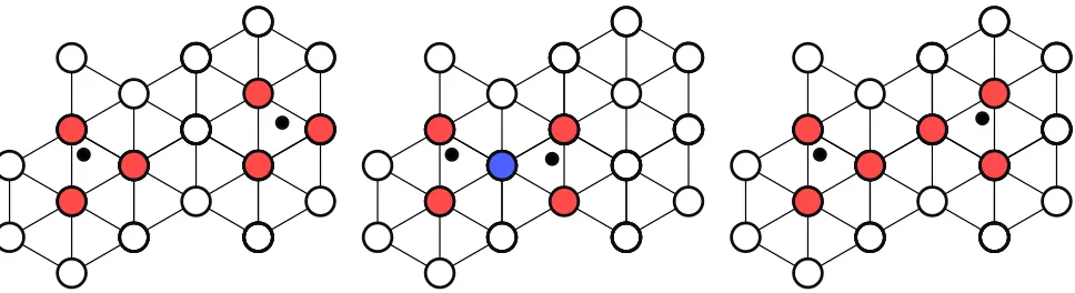
Fig. 1. Example of counting failure due to target positioning. Black filled nodes are targets, other nodes are sensors. White sensors count zero targets, red count one, and blue count two. The overall count is correct in the two leftmost examples, respectively because the two targets are separately detected (they are far enough) and because they are detected together (they are close enough). The enumeration fails on the rightmost example, because the two targets cannot be detected as two separate objects by any of the sensors.

the appropriate level set). Since no identity or position is associated with a target, they become impossible to distinguish from a local, purely topological point of view. In this section, we investigate the practical implica-tions of varying network densities, shapes, and the ratios between the communication and target detection ranges.

A. Experimental setup

We run our experiments in a square arena of 10x10m into which we deploy randomly-placed targets, and sen-sors with four different displacements: a regular and a perturbed square grid, and a regular and a perturbed hexagonal grid. We vary geometrically both the device density (from 0.04devices_m2 to20

devices

m2 ) and the number

of targets to track (from 1 to 100). We reduce the communication range with the square root of the device density increase, guaranteeing that the overall network shape stays similar regardless of the number of sensors deployed. We tune the parameters so that the commu-nication range is sufficient for the square grid to have a Moore neighbourhood, and for the hexagonal grid to have six neighbours for any sensor not on the network edge. Figure 2 depicts the different displacements, along with their communication links. We test each scenario with multiple values of target detection ranges: 1₄, 1₂,

3 4, 1,

3

2, and 2 times the communication range. We call

this the sensing/communication ratio (SCR). We let the simulation progress until all the sensors yield a stable value, and we measure the average normalised root mean square error (RMSE), defined as:

ERM S =

PN d=0(

T−cd

T ) 2

N

where N is the number of devices, T the number of targets, and cd the actual target count at device d. We

run our experiments on the Alchemist simulator [16].

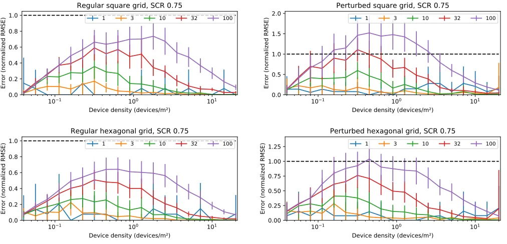
B. Device density and network shape

Raising the network density is not immediately bene-ficial, as depicted in Figure 3. The issue, shown in Fig-ure 1, is the root cause of this somewhat counter-intuitive behaviour: counting initially gets worse with higher

sensor densities, and then starts declining. With low device densities, in fact, there is a high chance that one or more sensors sees all the targets that have been deployed, and with very high densities there is an increasing chance of detecting the “emptyness” surrounding a single target – and consequently a high chance of being able to tell it apart from others. This consideration can be reflected in terms of target spatial distribution: tightly-packed targets or very sparse targets are easier to count. Device distri-bution is also relevant to the algorithm, as it may create disruptions in the simplicial complex structure. Perturbed grids both perform worse than their regular counterparts. On the other hand, different regular network structures do not influence the algorithm badly: counting errors are comparable between square and hexagonal grids.

C. Sensing/Communication range ratio

(8)

[image:8.612.65.552.49.165.2]

Fig. 2. Simulation screenshots. From left to right: regular square grid, perturbed square grid, regular hexagonal grid, perturbed hexagonal grid. Pink dots are targets, other dots are sensors. Colour indicates the number of targets sensed: red if none, blue if a single one, green if two.

10 1 ₁₀0 ₁₀1

Device density (devices/m²) 0.0

0.2 0.4 0.6 0.8 1.0

Error (normalized RMSE)

Regular square grid, SCR 0.75

1 3 10 32 100

10 1 ₁₀0 ₁₀1

0.5 1.0 1.5 2.0

Perturbed square grid, SCR 0.75

1 3 10 32 100

10 1 ₁₀0 ₁₀1

0.2 0.4 0.6 0.8 1.0

Regular hexagonal grid, SCR 0.75

1 3 10 32 100

10 1 ₁₀0 ₁₀1

0.25 0.50 0.75 1.00 1.25

Perturbed hexagonal grid, SCR 0.75

1 3 10 32 100

Fig. 3. Counting error against sensor density for different target counts (coloured lines) and different device displacements. Each point is the mean of 20 simulation runs, error bars show mean ±standard deviation. A 100% estimation error is marked with a black dashed line. The algorithm works well with regular networks and extreme sensor densities. The higher the number of targets to track, the higher the probability that the algorithm incurs the issue depicted in Figure 1

that also minimises the overlap between sensing regions. Raising the value further causes irregular networks to badly fail at counting.

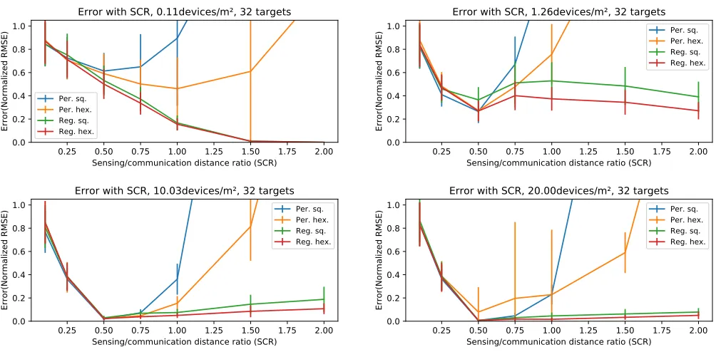
D. Recommendations

The above results show that for regular networks of carefully-placed sensors the Euler integration approach works very well. However, the approach has been shown to be sensitive to the regularity of the network, to its density, and to the ratio between the sensing and com-munication ranges. Particular attention must therefore be devoted to choosing a proper sensor density for the target system, as intermediate choices would spoil the counting.

In the case that the sensor comes with a fixed sensing range, and where this is wider than its communication range, then significant care is required in the spatial arrangement of the devices.

[image:8.612.55.561.223.467.2]

(9)

0.25 0.50 0.75 1.00 1.25 1.50 1.75 2.00 Sensing/communication distance ratio (SCR)

0.0 0.2 0.4 0.6 0.8 1.0

Error(Normalized RMSE)

Error with SCR, 0.11devices/m², 32 targets

Per. sq. Per. hex. Reg. sq. Reg. hex.

0.0 0.2 0.4 0.6 0.8 1.0

Error with SCR, 1.26devices/m², 32 targets Per. sq. Per. hex. Reg. sq. Reg. hex.

0.0 0.2 0.4 0.6 0.8 1.0

Fig. 4. Counting error against sensing/communication range ratio (SCR) for different sensor densities and 32 targets to count. Different sensor displacements are depicted in different colours. Each point is again the mean of 20 simulation runs, error bars show mean±standard deviation. Higher SCR can be beneficial for regularly-shaped networks, but very detrimental for irregular ones. A “sweet spot” can be identified around 0.5/0.75: at this ratio, there is maximum coverage of the space with minimum overlapping.

E. Comparison with other work

Perhaps the most comparable work in the literature on target counting is that of Gandhi at alia [5], which uses geometrical and statistical techniques to generate a minimal set of non-redundant sensors. A sensor is redundant if removing it does not remove coverage of a point in the space under observation. This approach clearly reduces the number of possible duplicate obser-vations (since it reduces the number of sensors observing common locations), and indeed the authors derive an estimate for the number of targets given (in our notation) by:

ˆ

Nt=

P ph(p)

√ m

wherepranges over the set of non-redundant sensors and m is the maximum degree of overlapping observations for any point in the space under observation. The actual target count is then constrained to lie within the range

ˆ Nt √

m,Nˆt

√ m

.

We note that, while this technique usesmas a minimal value for overlap, the Euler integration technique has a maximally-dimensionedk-simplex, the dimension of the complex as a whole. While not the same value, they seem

sufficiently close to suggest that similar bounds could be derived for the Euler integration technique – with the significant benefit of then requiring less geometric information and no redundancy-elimination step (which is a global operation). This is a topic we are interested in pursuing further.

V. CONCLUSION

In this paper we have presented a fully distributed and self-stabilising implementation of the Euler integration algorithm for counting unidentifiable targets in a wire-less sensor network. The implementation is written in the practical aggregate programming language Protelis, an implementation the higher-order field calculus. This programming paradigm provides a very straightforward way to compactly write fully-distributed algorithms that leverage the topological features of the sensor network. We evaluated the performance of the algorithm in several network configurations, varying sensor density, displace-ment, and sensing capabilities, and from our results drew some recommendations for the actual usage of integration-based counting.

[image:9.612.55.557.53.300.2]

(10)

targets. We would emphasise two further corollaries of this observation. Firstly, the approximation is sensitive to counting errors in the sensors themselves – and such errors are unavoidable, especially in long-lived systems as sensors degrade mechanically. Secondly, the coverage can be changed by sensor movement, failure, occlusion, and other factors. We have accounted for neither of these factors in our work: neither is at present well-understood, and both require significantly more research if we are to build systems that are robust to the real-world challenges to sensor systems.

There is also clearly a relationship between the num-ber of sensors that potentially observe a target (rep-resented by the order of the k-simplices representing their co-observation) and the redundancy of information within the system. One might imagine that higher-order simplices might indicate an opportunity to turn off some nodes in order to save battery power – although doing so then changes both the topology of the complex and the density of sampling, and therefore invites the problems observed above. More work is needed to explore these issues, but they potentially offer a mathematically well-founded way to adapt sensor behaviour without compro-mising data quality – or, perhaps more accurately, while allowing the data quality compromise to be calculated.

Acknowledgements

The work underlying this paper occurred during a visit the second author made to Cesena, and is par-tially supported by the UK EPSRC under grant number EP/N007565/1, “Science of Sensor Systems Software”.

Additional material

All the code and simulation material used in this paper can be obtained from a public reposi-tory available at https://bitbucket.org/danysk/experiment-2017-saso-counting.

REFERENCES

[1] Y. Baryshnikov and R. Ghrist, “Target enumerationn via integra-tion over planar sensor networks,” inProceedings of Robotics: Science and Systems IV, June 2009.

[2] ——, “Target enumeration via Euler characteristic integrals,” SIAM Journal of Applied Mathematics, vol. 70, no. 3, pp. 825–844, 2009. [Online]. Available: http://dx.doi.org/10.1137/070687293

[3] M. Viroli, J. Beal, F. Damiani, and D. Pianini, “Efficient engi-neering of complex self-organising systems by self-stabilising fields,” inSelf-Adaptive and Self-Organizing Systems (SASO), 2015 IEEE 9th International Conference on. IEEE, Sept 2015, pp. 81–90.

[4] D. Wu, B. Zhang, H. Li, and X. Cheng, “Target coutning in wireless sensor networks,” in The art of wireless sensor networks, volume 2: Advanced topics and applications, H. Am-mari, Ed. Springer-Verlag, 2014.

[5] S. Gandhi, R. Kumar, and S. Suri, “Target counting under min-imal sensing: Complexity and approximations,” inAlgorithmic aspects of wireless sensor networks, S. Fekete, Ed. Springer-Verlag, 2008, pp. 30–42.

[6] S. Guo, T. He, M. Mokbel, J. Stankovic, and T. Abdelzaher, “On accurate and efficient statistical counting in sensor-based surveillance systems,”Pervasive and Mobile Computing, vol. 6, no. 1, pp. 74–92, February 2010. [Online]. Available: https://doi.org/10.1016/j.pmcj.2009.07.013

[7] J. Beal, M. Viroli, D. Pianini, and F. Damiani, “Self-adaptation to device distribution changes,” in10th IEEE International Con-ference on Self-Adaptive and Self-Organizing Systems, SASO 2016, Augsburg, Germany, September 12-16, 2016, G. Cabri, G. Picard, and N. Suri, Eds., 2016, pp. 60–69, Best paper of IEEE SASO 2016. DOI: 10.1109/SASO.2016.12.

[8] D. Pianini, M. Viroli, and J. Beal, “Protelis: practical aggregate programming,” in Proceedings of the 30th Annual ACM Symposium on Applied Computing, Salamanca, Spain, April 13-17, 2015, 2015, pp. 1846–1853. [Online]. Available: http://doi.acm.org/10.1145/2695664.2695913

[9] J. Beal, D. Pianini, and M. Viroli, “Aggregate programming for the Internet of Things,” IEEE Computer, vol. 48, no. 9, pp. 22–30, 2015.

[10] J. Beal, M. Viroli, and F. Damiani, “Towards a unified model of spatial computing,” in7th Spatial Computing Workshop (SCW 2014), AAMAS 2014, Paris, France, May 2014.

[11] H. Edelsbrunner, A short course in computational geometry and topology, ser. SpringerBriefs in Applied Sciences and Technology. Springer, 2014. [Online]. Available: doi://10.1007/978-3-319-05957-0

[12] M. Viroli, G. Audrito, F. Damiani, D. Pianini, and J. Beal, “A higher-order calculus of computational fields,” CoRR, vol. abs/1610.08116, 2016. [Online]. Available: http://arxiv.org/abs/1610.08116

[13] J. Beal, D. Pianini, and M. Viroli, “Aggregate

programming for the internet of things,” IEEE Computer, vol. 48, no. 9, pp. 22–30, 2015. [Online]. Available: http://dx.doi.org/10.1109/MC.2015.261

[14] M. Viroli, J. Beal, F. Damiani, and D. Pianini, “Efficient engineering of complex organising systems by self-stabilising fields,” in2015 IEEE 9th International Conference on Self-Adaptive and Self-Organizing Systems, Cambridge, MA, USA, September 21-25, 2015, 2015, pp. 81–90. [Online]. Available: http://dx.doi.org/10.1109/SASO.2015.16

[15] M. Francia, D. Pianini, J. Beal, and M. Viroli, “Towards a foundational api for resilient distributed systems design,” in 2017 IEEE 11th International Conference on Self-Adaptive and Self-Organizing Systems, Tucson, AZ, USA, September 18-22, 2017, 2017, submitted for publication.