Playing Tic-Tac-Toe Using Genetic Neural
Network with Double Transfer Functions
Sai Ho Ling1, Hak Keung Lam2 1
Faculty of Engineering and Information Engineering, University of Technology Sydney, New South Wales, Australia; 2Division of Engineering, King’s College London, London, UK.
Email: [email protected], [email protected]
Received October 4th, 2010; revised November 3rd, 2010; accepted January 4th, 2011
ABSTRACT
Computational intelligence is a powerful tool for game development. In this paper, an algorithm of playing the game Tic-Tac-Toe with computational intelligence is developed. This algorithm is learned by a Neural Network with Double Transfer functions (NNDTF), which is trained by genetic algorithm (GA). In the NNDTF, the neuron has two transfer functions and exhibits a node-to-node relationship in the hidden layer that enhances the learning ability of the network. A Tic-Tac-Toe game is used to show that the NNDTF provide a better performance than the traditional neural network does.
Keywords: Game, Genetic Algorithm, Neural Network
1. Introduction
Games such as Backgammon, Chess, Checkers, Go, Othello and Tic-Tac-Toe are widely used platforms for studying the learning ability of and developing learning algorithms for machines. By playing games, the machine intelligence can be revealed. Some techniques of artifi-cial intelligence, such as the brute-force methods and knowledge-based methods [1], were reported. Brute- force methods, e.g. retrograde analysis [2] and enhanced transposition-table methods, solve the game problems by constructing databases for the games. For instance, the database is formed by a terminal position [2]. The best move is then determined by working backward on the constructed database. For knowledge-based methods, the best move is determined by searching a game tree. For games such as Checkers, the tree spanning is very large. Tree searching will be time consuming even for a few plies. Hence, an efficient searching algorithm is an im-portant issue. Some searching algorithms, which are classified as knowledge-based methods, are threat-space search and -search, proof-number search [3], depth-first proof-number search and pattern search.
It can be seen that the above game-solving methods depend mainly on the database construction and search-ing. The problems are solved by forming a possible set of solutions based on the endgame condition, or searching for the set of solutions based on the current game
condi-tion. The machine cannot learn to play the games by it-self. Unlike an evolutionary approach in [1], neural net-work (NN) was employed to evolve and to learn for playing Tic-Tac-Toe without the need of a database. Evolutionary programming was used to design the NN and link weights. A similar idea has been applied in a Checkers game [4-7]. Other games such as Backgammon [8], Othello [9] and Checkers [10] applying NNs or computational intelligence techniques can also be found.
This paper is organized as follows. An algorithm to evaluate each move on playing the Tic-Tac-Toe will be proposed in section 2. NNDTF will be presented in sec-tion 3. Genetic Algorithm will be presented in secsec-tion 4. Training of the NNDTF using GA to learn the rules of Tic-Tac-Toe will be presented in section 5. An example on playing Tic-Tac-Toe will be given in section 6. A conclusion will be drawn in section 7.
2. Algorithm for Playing Tic-Tac-Toe
The game Tic-tac-toe, also known as naughts and crosses, is a two-player game. Each player will place a marker, “X” for the first player and “O” for the second player, in turn in a three-by-three grid area. The first player takes the first move. The goal is to place three markers in a line of any direction on the grid area.
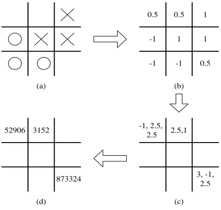
An algorithm is proposed in this section to evaluate the move on each grid. An “X” and an “O” on a grid are de-noted by 1 and –1 respectively. An empty grid is dede-noted by 0.5. The following procedure is used to evaluate each possible move.
1) Place an “X” on an empty grid.
2) Corresponding to step 1, sum up all the grid values for each line in any direction, e.g., for a grid in the corner, we have three evaluated values because there are three lines to win or lose.
3) Remove the “X” placed in step 1 and place an “X” on another empty grid. Evaluate this grid using the algo-rithm in step 2. Repeat this process till all empty grids are evaluated.
4) After evaluation, each grid will have been assigned at least 2 evaluated values for all possible lines, e.g. the center grid will have 4 evaluated values, corner grids will have 3 evaluated values and other grids will have 2 eva-luated values. There are totally 6 possible evaeva-luated val-ues: 3 (1 + 1 + 1), 2.5 (1 + 1 + 0.5), 2 (1 + 0.5 + 0.5), 1 (–1 + 1 + 1), 0.5 (–1 + 1 + 0.5) and –1 (–1 – 1 + 1). The most important evaluated value of a grid is 3, which in-dicts a winning of the game (3 “X”s in a line) if you put an “X” on that grid. The priority of taking that move is the highest. The second important evaluated value of a grid is –1 (2 “O”s and 1 “X” in a line), which indicts that the opponent should be prevented from winning the game. The priority of taking that move is the second highest. Using this rationale, the list of priority in a descending order is: 3, –1, 2.5, 2, 1, 0.5. Based on these assigned eva-luated values, a score will be assigned to each possible move. First, each evaluated value is assigned a score:
7 6 5 4
6 5 4 3
3 7 , 1 6 2 5, . 5 2, 4 ,
3 2
1 3 and 0 5. 122, The chosen scores have
the following properties,
6 4 5
(1)
5 4 4
(2)
4 4 3
(3)
3 4 2
(4)
2 4 1
(5) The sum of the scores of a grid is the final score. The final scores will be used to determine the priorities of the possible move. A higher final score of a grid indicates a higher priority of that move. The reasons for choosing the scores in this way with the properties of (1) to (5) are as follows. As the evaluated value of 3 indicates a win-ning of the game (3 “X”s in a line), the score of 6
must be the highest. There are at most four evaluated values for a grid. Hence, 6 must be greater than 4
times the second largest evaluated values, i.e. 45.
Consequently, the priority of a grid having an evaluated score with a higher priority will not be affected by other lower evaluated scores. For instance, consider a grid having evaluated values of 3 and 0.5, and another grid having evaluated values of 1, 2.5, 2 and 0.5. The final score of the former grid (77 + 22) is bigger than and latter grid (77 + 22 and 66 + 55 + 44 + 22). Thus, the “X” should be place at the grid having an evaluated value of 3 to win the game.
Take the game as shown in Figure 1 as an example, we have 3 “X”s and 3 “O”s. The next move will be to place an “X”. After assigning an empty grid to be 0.5, an “X” to be 1, an “O” to be –1, Figure 1(b) is obtained. Following Step 1 to Step 3, we obtain the evaluated val-ues as shown in Figure 1(c). Based on Step 4, Figure 1(d) shows the final scores for the empty grids. As the highest score is 873324, the most appropriate move is to put an “X” on the bottom right corner. This move not
0.5 0.5 1
1 1 -1
-1 -1 0.5
-1, 2.5, 2.5 2.5,1 52906 3152
873324 3, -1,
2.5
(a) (b)
[image:2.595.315.532.490.697.2](d) (c)
only lines up 3 “X”s to win a game, but also prevents the opponent to line up 3 “O”s. The second appropriate move, indicted by the final score of 52906, can gain a chance to win by lining up 2 “X”s, and prevent the op-ponent to win.
3. Neural Network with Double Transfer
Functions (NNDTF)
[image:3.595.312.536.91.302.2] [image:3.595.308.537.378.460.2]NN was proved to be a universal approximator [12]. A 3-layer feed-forward NN can approximate any nonlinear continuous function to an arbitrary accuracy. NNs are widely applied in areas such as prediction, system mod-eling and control [12]. Owing to its particular structure, a NN is good in learning [2] using some learning algo-rithms such as GA [1] and back propagation [2]. In gen-eral, the processing of a traditional feed-forward NN is done in a layer-by-layer manner. In this paper, by intro-ducing a node-to-node relationship in the hidden layer of the NN, a better performance can be obtained.
Figure 2 shows the proposed neuron. It has two acti-vation transfer functions to govern the input-output rela-tionships of the neuron: static transfer function (STF) and dynamic transfer function (DTF). For the STF, the para-meters are fixed and its output depends on the inputs of the neuron. For the DTF, the parameters of the activation transfer function depend on the outputs of other neurons and its STF. With this proposed neuron, the connection
of the proposed NN is shown in Figure 3, which is a
three-layer NN. A node-to-node relationship is intro-duced in the hidden layer. Comparing with the traditional feed-forward NN [12], it was reported in [13] that the proposed NN can offer a better performance and need fewer hidden nodes. The details of the NNDTF are pre-sented as follows.
3.1. The Neuron Models
We consider the STF first. Let vij be the synaptic
con-nection weight from the i-th input component xito the
j-th neuron. The output jof the j-th neuron’s STF is
defined as,
jth neuron ) ( j s net ) ( j d net 1 x 2 x in n
x j
j j p , 1 j j p , 1 1 j z 1 j z j v1 j v2 j nin v j z STF DTF
Figure 2. Model of the proposed neuron.
1 x 2 x in n x 1 2 h n 1 y 21 p 12 p 2 h n
p p2nh 1 h n p h n p1 11 v 12 v h n v1 h inn n v 2 in n v 1 in n v 11 w 21 w 1 h n w 1 z 2 z h n z out n w1 out n y out n w2 out hn n w h n
p1 nh1
[image:3.595.93.252.581.703.2]p
Figure 3. Connection of the NNDTF.
1
in
n j
j s i ij i
net x v
(6)wherei1 2, ,, nin, j1 2, ,, nh;nindenotes the
number of input and j
s
net is a static activation trans-fer function. The activation transtrans-fer function is defined as, 2 1 2 2 1 2 2 1 1 2 1 1 nin j i ij s i in j s in nin j
i ij s i
j s
x v m
n
n i ij s
j
i s i ij
i
x v m
e if x v m
net x v
e otherwise
(7)where j
s
m and j s
are the static mean and static stan-dard deviation for the j-th STF respectively. The
para-meters ( j
s
m and j s
) are fixed after the training
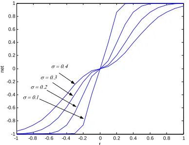
processing. Thus, the activation transfer function is static. The output of the STF depends on the inputs of the neu-ron only. From (7), the output value is ranged from –1 to 1. The shape of the proposed activation transfer function is shown in Figure 4 and Figure 5. It can be observed from these 2 figures that net f
1as f and
1net f asf .
Considering the DTF, the neuron output zj of the
j-th neuron is defined as,
j j j
j d j d d
z net ,m , (8)
where netdj
is the DTF defined as follows,
2 2 2 2 2 2 1 1 j j d j d j j d j d m j j dj j j
d j d d
m
e if m
net ,m ,
-1 -0.8 -0.6 -0.4 -0.2 0 0.2 0.4 0.6 0.8 1 -1
-0.8 -0.6 -0.4 -0.2 0 0.2 0.4 0.6 0.8 1
net
f m=-0.4
m=-0.2 m=0
[image:4.595.76.267.85.235.2]m=0.2 m=0.4
Figure 4. Sample transfer functions of the proposed neuron
( = 0.2).
-1 -0.8 -0.6 -0.4 -0.2 0 0.2 0.4 0.6 0.8 1
-1 -0.8 -0.6 -0.4 -0.2 0 0.2 0.4 0.6 0.8 1
f
net
[image:4.595.315.541.217.331.2]
Figure 5. Sample transfer functions of the proposed neuron (m = 0).
where
1 1
j
d j , j j
m p z (10)
1 1
j
d pj , j zj
(11)
j d
m and j d
are the dynamic mean and dynamic standard
deviation for the j-th DTF. zj1 and zj1 represent the
output of thej1-th and j1- th neurons respectively.
1 j , j
p denotes the weight of the link between the
1- th
j node and the j-th node and pj1, j denotes the
weight of the link between the j1- th node and the - th
j node. It should be noted that if j1, pj1, jis
equal to h
n , j
p and if jnh, pj1, j is equal to p1, j. In
this DTF, unlike the STF, the activation transfer function is dynamic as the parameters of its activation transfer
function depend on the outputs of the j1- th and
1- th
j neurons. Referring to (14), the input-output
relationship of the proposed neuron is as follows,
1
in
n
j j j j
j d s i ij d d
i
z net net x v ,m ,
(12)3.2. Connection of the NNDTF
As shown in Figure 3, the NNDTF has three layers with
in
n nodes in the input layer, nhnodes in the hidden
layer, and nout nodes in the output layer. In the hidden
layer, the neuron model presented in the previous section is employed. The output value of the hidden node de-pends on the neighboring nodes and input nodes. In the output layer, a static activation transfer function is em-ployed. Considering an input-output pair (x,y) , the output of the j- th node of the hidden layer is given by
1
in
n j j
j d s i ij
i
z net net x v
(13)The output of the NNDTF is defined as,
1
out
n l
l o j jl l
y net z w ,
l1 2, , , nout (14)1 1
out in
n n
l j j
o d s i ij jl
l i
net net net x v w
(15)where wjl denotes the weight of the link between the
- th
j hidden and the - thl output nodes; l
o
net
denotes the activation transfer function of the output neuron. The transfer function of the output node is de-fined as follows,
2
2
2
2
2
2
1
1 l k o l o
l k o l o
z m
l k o l
o j
z m
e if z m
net z
e otherwise
(16)
where l
o
m and l o
are the mean and the standard devia-tion of the output node activadevia-tion transfer funcdevia-tion re-spectively. The parameters of the NNDTF can be trained by GA [11].
4. Genetic Algorithm
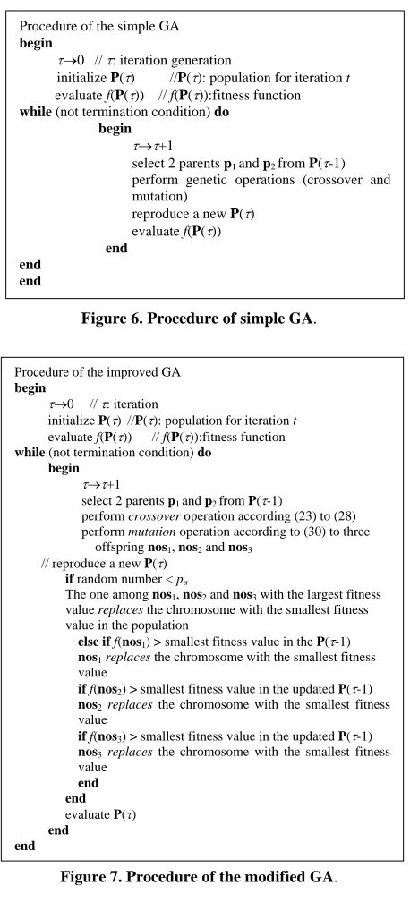
Genetic algorithms (GAs) are powerful searching algo-rithms. The traditional GA process [14-16] is shown in
Figure 6. First, a population of chromosomes is created. Second, the chromosomes are evaluated by a defined fitness function. Third, some of the chromosomes are selected for performing genetic operations. Forth, genetic operations of crossover and mutation are performed. The produced offspring replace their parents in the initial population. This GA process repeats until a user-defined criterion is reached. In this paper, the traditional GA is modified and new genetic operators [11] are introduced to improve its performance. The modified GA process is shown in Figure 7. Its details will be given as follows.
4.1. Initial Population
[image:4.595.78.272.277.426.2]Figure 6. Procedure of simple GA.
Figure 7. Procedure of the modified GA.
first set of population is usually generated randomly.
1 2 pop _ size
P p , , , p p (17)
1 2 j no _ vars
i pi pi pi pi
p , i1 2, ,,
1 2
pop _ size; j , ,,no _ vars (18)
j
j j
min i max
para p para (19)
where pop_size denotes the population size; no_vars denotes the number of variables to be tuned;
j
i
p ,
1 2
i , ,, pop_size; j1 2, ,, no_vars, are the parameters to be tuned; paraminj and
j max
para are the
minimum and maximum values of the parameter j
i
p
for all i. It can be seen from (17) to (19) that the poten-tial solution set P contains some candidate solutions pi
(chromosomes). The chromosome pi contains some
variables pi (genes).
4.2. Evaluation
Each chromosome in the populati on will be evaluated by a defined fitness function. The better chromosomes will return higher values in this process. The fitness function to evaluate a chromosome in the population can be writ-ten as,
ifitness f p (20)
The form of the fitness function depends on the appli-cation.
4.3. Selection
Two chromosomes in the population will be selected to undergo genetic operations for reproduction by the me-thod of spinning the roulette wheel [16]. It is believed that high potential parents will produce better offspring (survival of the best ones). The chromosome having a higher fitness value should therefore have a higher chance to be selected. The selection can be done by as-signing a probability qi to the chromosome pi:
1i i pop _ size
j j
f q
f
p
p
, 1 2i , ,, pop _ size (21)
The cumulative probability ˆqi for the chromosome
i
p is defined as,
1 i
i j
j
ˆq q
(22)The selection process starts by randomly generating a nonzero floating-point number, d
0 1
. Then, the chromosome pi is chosen if qˆi1 d qˆi, 1 2i , ,,pop_size, and qˆ00. It can be observed from this se-lection process that a chromosome having a larger
if p will have a higher chance to be selected. Conse-quently, the best chromosomes will get more offspring, the average will stay and the worst will die off. In the selection process, only two chromosomes will be se-lected to undergo the genetic operations.
4.4. Genetic Operations
The genetic operations are to generate some new chro-mosomes (offspring) from their parents after the selec-tion process. They include the crossover and the mutaselec-tion operations.
Procedure of the simple GA
begin
0 // : iteration generation
initialize P() //P(): population for iteration t
evaluate f(P()) // f(P()):fitness function while (not termination condition) do
begin
+1
select 2 parents p1 and p2 from P(-1) perform genetic operations (crossover and mutation)
reproduce a new P()
evaluate f(P()) end
end end
Procedure of the improved GA
begin
0 // : iteration
initialize P() //P(): population for iteration t
evaluate f(P()) // f(P()):fitness function
while (not termination condition) do begin
+1
select 2 parents p1 and p2 from P(-1)
perform crossover operation according (23) to (28) perform mutation operation according to (30) to three
offspring nos1, nos2 and nos3 // reproduce a new P()
if random number < pa
The one among nos1, nos2 and nos3 with the largest fitness value replaces the chromosome with the smallest fitness value in the population
else if f(nos1) > smallest fitness value in the P(-1)
nos1 replaces the chromosome with the smallest fitness value
if f(nos2) > smallest fitness value in the updated P(-1)
nos2 replaces the chromosome with the smallest fitness value
if f(nos3) > smallest fitness value in the updated P(-1)
nos3 replaces the chromosome with the smallest fitness value
end end
evaluate P()
[image:5.595.65.284.607.689.2]4.4.1. Crossover
The crossover operation is mainly for exchanging infor-mation from the two parents, chromosomes p1 and p2,
obtained in the selection process. The two parents will produce one offspring. First, four chromosomes will be generated according to the following mechanisms,
1 1 1 1 1 2
1 2
2
c os os osno _ vars
p p
os (23)
2 2 2 2
1 2
max 1 max 1 2 c os os osno _ vars
w , w
os
p p p
(24)
3 3 3 3
1 2
min 1 min 1 2 c os os osno _ vars
w , w
os
p p p
(25)
4 4 4 4
1 2
max min 1 1 2
2
c os os osno _ vars
w w
os
p p p p
(26)
1 2
max max max max
no _ vars
para para para
p (27)
1 2
min min min min
no _ vars
para para para
p (28)
where w
0 1
denotes a weight to be determined by users, max
p p1, 2
denotes a vector with each elementobtained by taking the maximum among the correspond-ing element of p1 and p2. For instance,
max 1 2 3, 2 3 1 2 3 3 . Similarly,
1 2
min p p, gives a vector by taking the minimum
val-ue. For instance, min 1
2 3
,2 3 1
1 2 1
. Among 1
c
os to 4 c
os , the one with the
largest fitness value is used as the offspring of the cros-sover operation. The offspring is defined as,
1 2
ios
no _ var s c
os os os
os os (29)
where ios denotes the index i which gives a maximum
value of
ic
f os , 1 2 3 4i , , , .
If the crossover operation can provide a good offspring, a higher fitness value can be reached in less iteration. As seen from (23) to (26), the offspring spreads over the domain: (23) and (26) will move the offspring near cen-tre region of the concerned domain (as w in (26) ap-
proaches 1, osc4 approaches 1 2
2
p p
), and (24) and (25)
will move the offspring near the domain boundary (as w
in (24) and (25) approaches 1, 2
c
os and 3
c
os
approach-es pmax and pmin respectively). The chance of getting
a good offspring is thus enhanced.
4.4.2. Mutation
The offspring (30) will then undergo the mutation opera-tion. The mutation operation is to change the genes of the
chromosomes. Consequently, the features of the chro-mosomes inherited from their parents can be changed. Three new offspring will be generated by the mutation operation:
1 2
1 1 2 2
j no _ var s
no _ var s no _ var s
os os os
b nos b nos b nos
nos
(30)
where b , ii 1 2, ,, no _ vars, can only take the value of 0 or 1; nosi, i1 2, ,, no _ vars, are randomly
generated numbers such that paramini osij nosi i
max
para
. The first new offspring (j 1) is obtained
according to (30) with that only one bi (i being
ran-domly generated within the range) is allowed to be 1 and all the others are zeros. The second new offspring is ob-tained according to (30) with that some randomly chosen bi are set to be 1 and others are zero. The third new offspring is obtained according to (30) with all bi 1. These three new offspring will then be evaluated using the fitness function of (21). A real number will be gener-ated randomly and compared with a user-defined number
0 1
a
p . If the real number is smaller than pa, the
one with the largest fitness value fl among the three
new offspring will replace the chromosome with the
smallest fitness f in the population (even when
l s s
f f .) If the real number is larger than pa, the first offspring will replace the chromosome with the smallest fitness value fs in the population if fl fs ; the
second and the third offspring will do the same. pa is
effectively the probability of accepting a bad offspring in order to reduce the chance of converging to a local mum. Hence, the possibility of reaching the global opti-mum is kept.
We have three offspring generated in the mutation process. From (30), the first mutation (j 1) is in fact a uniform mutation. The second mutation allows some randomly selected genes to change simultaneously. The third mutation changes all genes simultaneously. The second and the third mutations allow multiple genes to be changed. Hence, the domain to be searched is larger as compared with a domain characterized by changing a single gene. As three offspring are produced in each generation, the genes will have a larger space for im-proving the fitness value when the fitness value is small. When the fitness values are large and nearly steady, changing the value of a single gene (the first mutation) may be enough as some genes may have reached the op-timal values.
reached.
5. Training of the NNDTF
In this section, the GA will be employed to train the pa-rameters of the NNDTF to play Tic-Tac-Toe based on the gaming algorithm in Section 2. The NNDTF with 9 inputs and 1 output is employed. The grids are numbered from 1 to 9 from right to left and from top to bottom. An “X” on the grid is denoted by 1, an “O” is denoted by –1, and an empty grid is denoted by 0.5. The grid pattern represented by numerical values will be used as the input of the NNDTF. The output of the NNDTF (y t
which a floating point number ranged from 1 to 9) represents the position of the marker that should be placed on. In order to have a legal move (place a marker on an empty grid), the marker is placed on an empty grid that has its grid number closest to the output of the network.To perform the training, we have to determine the pa-rameters to be trained and the fitness function describing the problem’s objective. The parameters of the modified network to be turned is
1 1
j j l l
ij s s j , j j , j jl o o
v m p p w m
for all i, j,l , which will be chosen as the chromosome for the GA. 100 different training patterns (obtained based on the proposed gaming algorithm stated in Sec-tion 2) are used to feed into the NNDTF for training. The fitness functions is designed as follows,
100
1 100
1 m i
max i
S y t , t
fitness
S t
x
x
(31)
where y t
denotes the output of the NNDTF with thet-th training pattern x
t as the input, Sm
y t ,
x t
denotes the final score for grid y t
and the t-thtrain-ing pattern x
t based on the gaming algorithm.
max
S x t denotes the maximum final score value
among all the empty grids for the t-th training pattern
tx . The GA is to maximize the fitness value (ranged
from 0 to 1) so as to force the output of the NNDTF to the grid number having the largest final score to ensure the best move.
6. Example
[image:7.595.309.536.111.177.2]In this session, a 9-input-1-output NNDTF is used for training. The number of hidden nodes is chosen to be 8. 100 training patterns are used for training with 50000 iterations. The population size, probability of acceptance, and w are chosen to be 10, 0.5 and 0.1, respectively. After training, the fitness value obtained is 0.9605. The upper and lower bounds of each parameter are 1 and –1,
Table 1. Results of the proposed NN playing Tic-Tac-Toe against with the traditional NN for 50 games.
Proposed NN
Wins: Draws: Loses
Proposed approach moves
first 18: 3: 4
Traditional approach
moves first 13: 4: 8
respectively. The initial values of the parameters are gen-erated randomly.
For comparison purposes, a traditional 3-layer feed- forward NN [17] trained by GA with arithmetic crossov-er and non-uniform mutation [17] is also applied undcrossov-er the same conditions to learn the gaming strategy in Sec-tion 2. The probabilities of crossover and mutaSec-tion are selected to be 0.8 and 0.1, respectively. The shape para-meter of the traditional GA for non-uniform mutation [17] is selected to be 5. These parameters are selected by trial and error for the best performance. After training for 50000 iterations, the fitness value obtained is 0.9456.
To test the performance of our proposed method, our trained NN plays Tic-Tac-Toe with the trained traditional NN for 50 games is carried out. The first 25 grid patterns, which are generated randomly with 2 “O”s and 2 “X”s, are the same as the next 25 grid patterns. For the first 25 games, the proposed approach moves first. For the second 25 games, the traditional approach moves first. The results are tabulated in Table 1. It can be seen that the proposed approach performs better. The number of wins is 18 by using NNDTF while only 13 by using the tradition NN.
7. Conclusions
A neural network with double transfer functions and trained with genetic algorithm has been proposed. An algorithm of playing Tic-Tac-Toe has been presented. A new transfer function of the neuron with a node-to-node relationship has been proposed. The proposed neural network is trained by genetic algorithm to learn the algo-rithm of playing Tic-tac-toe. As a comparison, the trained NN has played against the traditional NN trained by the traditional GA. The result has shown that the proposed approach performs better.
REFERENCES
[1] H. J. V. D. Herik, J. W. H. M. Uiterwijk and J. V. Rijs-wijck, “Games Solved: Now and in the Future,” Artificial
Intelligence, Vol. 134, No. 1-2, 2002, pp. 277-311. doi:10.
1016/S0004-3702(01)00152-7
[3] L. V. Allis, M. V. D. Meulen and. V. D. Herik, “Proof- Number Search,” Artificial Intelligence, Vol. 66, No.1, 1994, pp. 91-124. doi:10.1016/0004-3702(94)90004-3 [4] D. B. Fogel and K. Chellapilla, “Verifying Anaconda’s
Expert Rating by Competing against Chinook: Experi-ments in Co-Evolving a Neural Checkers Player,”
Neur-computing, Vol. 42, No. 1-4, 2002, pp. 69-86. doi:10.10
16/S0925-2312(01)00594-X
[5] K. Chellapilla and D. B. Fogel, “Evolving Neural Net-works to Play Checkers without Relying on Expert Knowledge,” IEEE Transactions on Neural Networks, Vol. 10, No. 6, 1999, pp. 1382-1391. doi:10.1109/72.80 9083
[6] K. Chellapilla and D. B. Fogel, “Evolving an Expert Checkers Playing Program without Using Human Exper-tise,” IEEE Transactions on Evolutionary Computation, Vol. 5, No. 4, 2001, pp. 422-428. doi:10.1109/4235.94 2536
[7] K. Chellapilla and D. B. Fogel, “Autonomous Evolution of Topographic Regularities in Artificial Neural Net-works,” Neural Computation, Vol. 22, No. 7, 2010, pp. 1860-1898. doi:10.1162/neco.2010.06-09-1042
[8] G. Tesauro, “Programming Backgammon Using Self- Teaching Neural Nets,” Artificial Intelligence, Vol. 134, No. 1-2, 2002, pp. 181-199. doi:10.1016/S0004-3702(01) 00110-2
[9] S. Y. Chong, M. K. Tan and J. D. White, “Observing the Evolution of Neural Networks Learning to Play the Game of Othello,” IEEE Transactions on Evolutionary
Compu-tation, Vol. 9, No. 3, 2005, pp. 422-428. doi:10.1109/TE-
VC.2005.843750
[10] D. E. Beal and M. C. Smith, “Random Evolutions in Chess,” ICCA Journal, Vol. 17, No. 1, 1994, pp. 3-9. [11] F. H. F. Leung, H. K. Lam, S. H. Ling and P. K. S. Tam,
“Tuning of the Structure and Parameters of Neural Net-work Using an Improved Genetic Algorithm,” IEEE
Trans-actions on Neural Networks, Vol.14, No. 1, 2003, pp. 79-
88. doi:10.1109/TNN.2002.804317
[12] M. Brown and C. Harris, “Neuralfuzzy Adaptive Model-ing and Control,” Prentice Hall, Upper Saddle River, 1994.
[13] S. H. Ling, F. H. F. Leung, H. K. Lam, Y. S. Lee and P. K. S. Tam, “A Novel GA-Based Neural Network for Short-Term Load Forecasting,” IEEE Transactions on
Industrial Electronics, Vol. 50, No. 4, 2003, pp. 793-799.
doi:10.1109/TIE.2003.814869
[14] J. H. Holland, “Adaptation in Natural and Artificial Sys-tems,” University of Michigan Press, Ann Arbor, 1975. [15] D. T. Pham and D. Karaboga, “Intelligent Optimization
Techniques, Genetic Algorithms, Tabu Search, Simulated Annealing and Neural Networks,” Springer-Verlag, New York, 2000.
[16] Z. Michalewicz, “Genetic Algorithm + Data Structures = Evolution Programs,” 2nd Edition, Springer-Verlag, New York, 1994.