Identifying Application Phases in Mobile Encrypted Network Traffic

1

Faculty of Electrical Engineering,

Mathematics & Computer Science

Identifying Application Phases

in Mobile Encrypted Network Traffic

Tycho Teesselink

Msc. Thesis

September 2019

Identifying Application Phases in Mobile Encrypted

Network Traffic

T. Teesselink

Enschede, Netherlands [email protected]

Abstract—Mobile devices have overtaken personal computers

for everyday tasks. These devices produce massive amounts of data which contains valuable information. Two fields in which monitoring of such mobile data is used are application identification and user action identification. They focus on the identification of a single user action or identify individual applications out of a known set. Monitoring this traffic can be useful for, among other things, fingerprinting traffic, intrusion detection and user-profiling. One limitation of previous works is that they are applicable for only a single user action or application. In this paper we generalise the concept of user actions by introducing mobile application phases. Application phases describe the state an application is in after a set of user actions have been performed. In contrast to user actions, these phases are application agnostic. This means that a method capable of classifying application phases is scalable and not limited to known applications. We formally define seven different application phases and show how to detect these in Android logs. We also present four different algorithms to detect these application phases in encrypted network traffic. We look at network traffic because it makes the method more scalable than a host-based solution and has a less privacy invasive nature. These algorithms use network data from a timeseries perspective instead of a flow perspective in order to take advantage of periods where network data is scarce. To assess the quality of these algorithms we generated two novel datasets consisting of encrypted network data of 361 Android applications. We were able to detect the installation of applications with 100% accuracy and distinguish foreground from background traffic with 93% accuracy.

I. INTRODUCTION

Device monitoring has been a topic of interest for several years with applications such as intrusion and extrusion detection [1], [2], application classification [3], [4] and user profiling [5]. Nowadays, personal computers are increasingly being replaced by mobile devices [6] due to the fact that smartphone computing power has increased significantly over the past few years. This means that people use their smartphones in favor of their personal computer for more and more tasks and generate massive amounts of mobile data. Monitoring solutions for desktop systems cannot be used for the mobile environment easily because they rely on implementation aspects specific to desktops. Mobile devices mostly use HTTPS to send their traffic, and use services like content delivery networks and APIs used by many applications. This has resulted in an increase in interest for the possibilities regarding the monitoring of traffic from these mobile devices.

There are two main methods for device monitoring. Host-based solutions require an application to be installed on the device, and therefore are intrusive, not scalable and sometimes even just not possible. The other method looks at the network traffic produced by the devices. This allows for more scalability as it only requires connectivity to the network access point and since most network traffic is encrypted nowadays, it is also less privacy invasive. Because of this reason we only focus on the network-based solutions.

Previous work has already shown that even though most mobile application traffic is encrypted nowadays, there are still methods in which information can be inferred [7]–[13]. Two important fields within network monitoring that have emerged are application identification and user action identification. The first group attempts to identify the application generating the network traffic (e.g. Facebook, Twitter or Instagram). The other group looks at identifying specific user actions for those applications in the network traffic. This includes actions such as sending an email, browsing Instagram photos or reading news. These fields provide information which can be used for many different purposes. Security operators can use the information for monitoring purposes and network load balancing, advertisement agencies can use this information for user profiling and targeted advertisement and even rogue individuals or governments can use the information to target specific applications or users.

The goal of this work is to explore and identify different application phases. Moreover, we aim to identify and classify these application phases in encrypted network traffic. This allows us to do monitoring for defensive purposes and usage statistics analysis. We motivate our work by outlining these use cases in which application identification can be used.

Defensive Monitoring— Intrusion detection systems (IDS) monitor all kinds of network traffic. When anomaly-based IDS encounter network traffic that was not modeled during it’s train-ing phase, it raises an alert. Therefore, many of these systems rely on a training phase which is as complete as possible. This entails that all applications that are going to be used within an environment need to be present in the training set in order to limit the number of false positives. One of the problems anomaly-based IDS cope with is dynamic environments. If an application is updated, the network environment changes or user habits change, the observed network behaviour can be different from what it looked like when the original model was created. This means that the model is also no longer accurate. This phenomenon where data distributions change over time is called concept drift [14]. Concept drift can result in many false alerts which have to be investigated manually. Using application phase data we can create a context model for these intrusion detection systems. E.g. if we detect the installation of a new application, we expect to see network traffic that is not yet modeled in our intrusion detection system. Normally, this would raise an alarm, however with the application phase context we might be able to more quickly resolve the issue, or even automatically learn a new model from the traffic that belongs to the new application.

Usage Statistics Analysis— An actor capable of observing network traffic could use application phase data to get a detailed profile of how an application is used by a specific user or a group of users. Analysis of mobile application usage is an important field in itself [15], [16]. They ask questions such as how long applications are used, how often they are used and at what time of day are they used. The answers to these questions are used to, among other things, help shape the development direction of the mobile application landscape and can be used in advanced recommendation systems [17]. Current methods mainly obtain this information by installing an application on the device itself. Installing a monitoring application on the device is not trivial as the party looking to obtain the usage statistics may have no access to the device. Application phase data obtained by only looking at the network traffic would therefore be very useful.

A. Contributions

In this work we generalise the concept of user actions to application phases. We identify these application phases in encrypted network traffic and learn a model capable of classifying unknown network traffic in these application phases.

Our contributions are as follows:

• We introduce mobile application phases and provide a

formal definition for them based on the identifiers used to detect them.

• We present an approach to classify mobile encrypted

network traffic in application phases. Our method looks at network traffic from a timeseries perspective instead of a flow perspective. We show how this approach is better suited for the problem of application phase classification.

• We captured a large dataset with encrypted mobile network

traffic on which we evaluate our approach.

II. MOBILEAPPLICATIONPHASES

In this work we are interested in mobile application phases. We provide an explanation of the application phases and give a formal definition for seven mobile application phases based on the identifiers used to detect them.

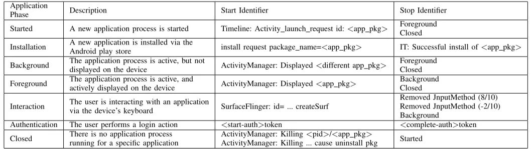
Android provides specific log messages related to changes in application phases. These messages identify the start of an application phase, or the end of it. We identify 7 different application phases and show how to detect them based on 11 different log messages. The application phases, a description, and the formal definition based on those log identifiers can be found in Table I.

Started— The started phase indicates that an application has been started, but it has not yet been displayed. This phase is only used for implementation purposes of the labelling system and is not a phase we predict. If an application is not active yet on the Android system, an activity for that application has to be started by issuing a view intent (usually the MainActivity). We detect this in the logs by looking for the ‘Timeline: Activity launch request id: <app pkg>’ message. Installation — The installation phase is defined by the process of installing a new application from the Google play store onto the device. The installation phase is important in helping to improve algorithms to deal with dynamic environments by providing a context and therefore crucial for the defensive monitoring use case. This phase includes all traffic produced between the start of the installation and the moment the installation process is finished.

In this work we introduce our own start and stop tokens to indicate the installation phase. We utilize the presence of the ‘install’ button in the Google Play store, which is only visible if the application is not installed on the Android device. After activating this button, we logged a message with an identifier in the form of <start-inst>. If the application was finished installing on the device, the ‘install’ button changes into two buttons with ‘Uninstall’ and ‘Open’ for that specific application. Therefore if we detected this button in the UI after initiating an installation process the process was complete, and as such a <stop-inst>identifier was logged. Alternatively the identifiers from the Google play store can be used, as listed in Table I.

TABLE I

APPLICATION PHASES AND THE IDENTIFIERS USED TO IDENTIFY THEM IN THE LOG. SOME APPLICATIONS DO NOT HAVE A STOP IDENTIFIER,BUT END WHEN A DIFFERENT APPLICATION PHASE IS STARTED

Application

Phase Description Start Identifier Stop Identifier

Started A new application process is started Timeline: Activity launch request id:<app pkg> Foreground_Closed

Installation A new application is installed via the_{Android play store} install request package name=<app pkg> IT: Successful install of<app pkg>

Background The application process is active, but not_{displayed on the device} ActivityManager: Displayed<different app pkg> Foreground_Closed

Foreground The application process is active, and_{actively displayed on the device} ActivityManager: Displayed<app pkg> Background_Closed

Interaction The user is interacting with an application_{via the device’s keyboard} SurfaceFlinger: id= ... createSurf Removed JnputMethod (8/10)Removed JnputMethod (-2/10) Background

Authentication The user performs a login action <start-auth>token <complete-auth>token

Closed There is no application process_{running for a specific application} ActivityManager: Killing_{ActivityManager: Killing ... cause uninstall pkg}<pid>/<app pkg> Started

For each application

Started Foreground

Closed Background

Interaction

Authentication

Start

Kill process Display

Open Keyboard

Kill p roce

ss

Resume

Close Keyboard Display

other KeybClose oa_rd

login done

Google Play Store

Installation Foreground

Background

Kill process Start

Display

Started

Closed

Install Done

Resume Display other Kill p

roce ss

Fig. 1. Visualisation of the state machines. Oval shapes are phases, where the arrows indicate possible state transitions between those phases.

When the Android phone tries to display an application that has previously been started it requests only a display intent for the activity and the activity does not have to be started again. We looked for the identifier that indicates an application starting phase, if the application was not yet started. Otherwise, we look for a display event in the logs and captured their corresponding log messages. The foreground phase can end in one of two ways. The first option is that another application is being displayed on the device, sending the application to the background. The other option is that the application is being closed. In that case we look for an identifier which indicates a closing action.

Background — We define an application to be in the

background phase if the application is active (e.g. it was previously started) but not being actively displayed on the device. This phase is also interesting for the usage statistics use case. However, it is also interesting for the defensive monitoring use case. An application that shows a lot of activity while it is in the background, might be indicative of malware. We detect that an application is in the background if we encounter a display event of a different activity (such as another application or the home screen). The background phase can end in two ways.

used to track user activity). In general this phase is beneficial for both the usage statistics and defensive monitoring use case. There is no default Android process or event that indicates that a user is logging into an application. We created a custom log message by logging a ‘start-authentication’ identifier and the corresponding timestamp when the login scripts were initiated. When the login scripts were finished, we logged a ‘complete-authentication’ identifier and the corresponding timestamp. Once the authentication phase is complete, the state machine transitions back to the foreground phase.

Closed — The closed phase is not neccessarily a phase we predict, as the phase is defined as having an application that is completely closed. This would mean that there is no activity currently running for that application on the device and no network data is being generated. This phase is used for implementation purposes of our labelling system (e.g. when an application is in the foreground, but it is being closed). When applications are being closed, the activity manager logs a specific message which indicates that the activity corresponding to that application is being killed. We captured all the log messages that contained the text ‘Activitymanager: killing’.

Another possibility is that Android is uninstalling an applica-tion. When an application is uninstalled, we saw a specific ‘kill’ message in the logs with the reason for why that application process was killed. For uninstalling this message was ‘pkg uninstall’. We logged the messages that contained this message as specifically a log message corresponding to ‘uninstalling an application’.

III. METHODOLOGY

The goal of this work is to identify mobile application phases in encrypted network traffic. Therefore, we first generate and label an encrypted mobile network traffic dataset. Second we describe our approach in which we train classifiers on labelled network traffic and subsequently classify unlabelled network traffic.

A. Mobile Network traffic

In our work we aim to identify application phases from a network traffic perspective. In order to observe those application phases we look at the network traffic produced by mobile applications. We focus specifically on mobile devices due to their dynamic nature. Mobile devices are much more mobile and evolutionary compared to personal computers. More applications are installed and devices leave and new devices enter the network. There is also less awareness regarding the security of mobile devices [18]. Most people have installed firewalls and anti-virus on their personal computer, but their mobile devices are left insecure. On top of that the majority of the network traffic generated worldwide originates from mobile devices [6].

Because nearly all mobile traffic is encrypted nowadays, the network traffic should be captured in it’s encrypted form. There are pre-existing datasets available that meet these criteria, however in order to evaluate the effectiveness of our classification method we require ground truth labels for the

network data. Because we introduced new application phase labels, these pre-existing datasets do not contain labels conform to our definintions as described in Table I. Applying such labels manually would be very hard, if not impossible because we do not have the system logs that correspond to that network traffic. To overcome this issue we generate a new encrypted mobile network dataset and label it accordingly.

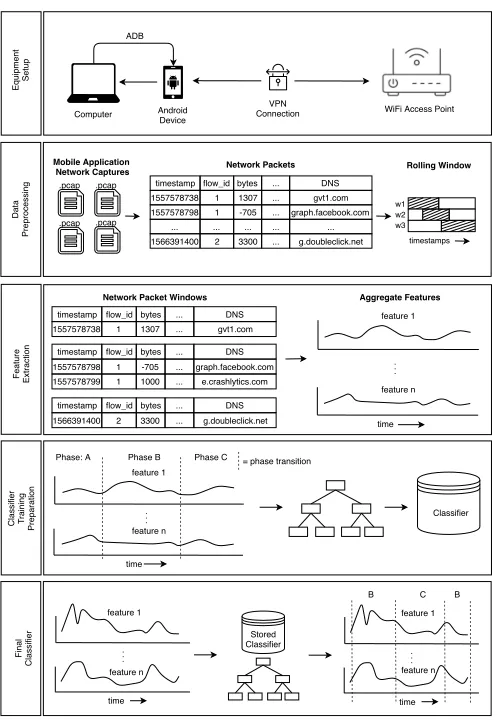
1) Equipment Setup: This section provides an overview of the setup we use to capture our network data. We first explain each of the components and then show how they interact with each other for the complete setup. An overview of the equipment setup is depicted in Figure 2.

The first component in the setup is the mobile device. In this work we focus on the Android operating system as it has the largest market share in the world [19]. However, any mobile device could be used if the phase identifiers are translated to that specific platform. We connect the Android device to the internet using a WIFI connection and we use a VPN connection from the device to our server, which allows us to capture the traffic that arrives on the specific interface belonging to that VPN. This ensures that we obtain network traffic which is less noisy. The Android device is also connected to a computer via usb cable. On that computer the Android Debug Bridge (ADB) is installed which enables us to send commands to the Android device and to read log output. Even though access to the Android device also allows us access to extra information which could be useful for classification purposes, we do not use any other information than the network traffic in order to keep our method non-intrusive and scalable.

2) Data Capture Implementation: The process of data capture is divided into three phases. During the process of capturing data, we also programmatically inspect the Android system logs using an Android system application called Logcat. Logcat is a command-line tool which dumps several Android logs containing system messages1_{. This tool writes specific}

log messages related to changes in application phases to an output file. An overview of the messages used to identify the phases is listed in Table I. The first step is to start a new network capture and commence the log dump. Next we install an application to the device and launch that application. This introduces installation phase traffic to our dataset. We then start to generate network traffic by performing touch interactions on the application using the Android monkey tool2_.

This tool is able to perform random touches and swipes on the device without the need for human interaction. We perform the interactions automatically because it allows us to capture data for a much larger group of applications compared to performing the interactions manually. Finally we uninstall the application from the phone in order to limit background noise originating from previously installed applications. We end the capture and record the name of the application in order to later retrace what traffic was generated by which application. The process

1_{Logcat tool, https://developer.Android.com/studio/command-line/logcat,}

Accessed 13-08-2019

2_{Android Monkey, https://developer.Android.com/studio/test/monkey.html,}

Stored Classifier

VPN Connection ADB

WiFi Access Point Computer Android Device Eq u ip me n t Se tu p time

Network Packet Windows

C la ssi fie r T ra in in g Pre p a ra ti o n feature 1 feature n . . . Classifier Final C la ssi fie r Data Pre p ro ce ssi n g F e a tu re Ext ra ct io n Network Packets Mobile Application Network Captures .pcap .pcap .pcap .pcap Rolling Window

timestamp flow_id bytes DNS 1557578738 1 1307 gvt1.com 1557578798 1 -705 graph.facebook.com

... ... ... ... 1566391400 2 3300 g.doubleclick.net

... ... ... ... ... ... ... ... ... ... timestamp flow_id bytes DNS 1557578738 1 1307 gvt1.com

1557578798 1 -705 graph.facebook.com 1557578799 1 1000 e.crashlytics.com

1566391400 2 3300 g.doubleclick.net ...

timestamp flow_id bytes DNS

... timestamp flow_id bytes DNS

feature 1 feature n . . . time feature 1 feature n . . .

Phase: A Phase B Phase C

time

Aggregate Features

= phase transition

feature 1 feature n . . . time B C B

timestamps w1 w2 w3

Fig. 2. Schematic overview our approach. We first show the network setup used for data capture. Next we extract information from the raw .pcap files and apply rolling windows to the network packets. Feature extraction is then applied on the network packet windows and labels are applied. Finally we train a classifier on the training data which is able to classify unlabelled network traffic.

of data capture is automated through a script and repeated for each application.

B. Labels

The labelling process works by ‘replaying’ and processing the Android system messages from the logs in chronological order. To keep track of the application phases, we start by creating two state machines for our system. These state machines represent the Android play store and the Android device itself. Figure 1 provides an overview of the possible states and transitions. The state machines have an internal timestamp which indicates the arrival time of the log entry that was processed last. Initially no applications are registered in the Android state machine and the Android play store is set to closed. We set the internal timestamp of the statemachines to the timestamp of the first observed packet and then iterate through the network packets we captured. If the timestamp of the observed packet is greater than the current timestamp of the statemachines, we need to process all messages observed in the

Android logs up to the timestamp of that network packet. We are reconstructing what the application phase of each application on the phone looked like, at the time of receiving the network packets.

We defined application phases in a way so that only one phase can be active at the same time. If all entries of the Android log are processed up to the timestamp of the packet, we extract the name and the phase of the application which is active at that specific moment. If the play store is active instead of an application, we extract it’s phase. This process is repeated for all network packets. The final output of the whole process is a set of tuples containing all the network packets with their corresponding application phase labels.

C. Data Preprocessing

In order for us to be able to learn classification models from our data, we need to process our raw network captures first. A schematic overview of the process is depicted in the ‘Data Preprocessing’ step in Figure 2. The network data we captured consists of pcap files. Our network data can be represented in different forms. In this work we considered two types; network flows and timeseries. A network flow is the combination of all traffic that belongs to the same tcp stream, where a tcp stream is identified by it’s 5-tuple (source IP and port, destination IP and port and the protocol). This type of representation is currently used in many application identification (e.g. [7], [20]), and user action identification papers (e.g. [8], [9]). Therefore the first step of our data proprocessing step consists of taking our raw network captures and extracting the network packets. In order to differentiate between incoming and outgoing packets we used positive and negative packet lengths. Packets that originated from the device were assigned a positive amount of bytes and packets that were received by the device were assigned a negative amount of bytes.

In comparison to other works, we do not try to assign classes to identifiable pieces of network data, but we try to classify a continuous application phase. Some application phases consist (partially) of an absense of data (e.g. background traffic). This means that if we classify based on flows, we can only classify observable data and cannot take advantage of an absense of network data. This can be seen from our dataset where there is 5.8 times as much foreground traffic as background traffic when using a flow perspective. This ratio changes to 2.5 when looking at the data from a timeseries perspective. This has to do with the fact that the background traffic is concentrated in a small amount of flows. By looking at the packets individually we do not limit ourselves to the information from the flow, but we can use the individual packets.

similar, however if you look at them in sequences, patterns start to appear in the data. To obtain sequences, we apply a rolling window to the packets. The size of the rolling window can be determined in several different ways. You can have a deterministic amount of datapoints per window, or you can use a timed rolling window. Because we want to look at sequences of packets taking into account their timing, we used a time based rolling window.

D. Feature Extraction

Several features have been introduced for our classification problem. We start with some of the limitations of encrypted network traffic and how we overcome this problem. We then go over each of the features and the intuition behind it, and finally show how we calculated them.

With the introduction of encryption, application data no longer holds textually valuable information. Therefore, classi-fication systems that rely on the payload of network packets (i.e. deep packet inspection) are no longer compatible. This has resulted in a shift from classification based on application payload to meta-data of network packets. We can still look at statistical properties of the packets we receive and identify patterns. There are many differrent possibilities regarding distributions of packet sizes, arrival times of packets, ratios between sent and received packets and total amount of traffic. In our work we look at several features that are extracted from such statistical features. This process is described in the ‘Feature Extraction’ step in Figure 2.

Count of unique active flows — This feature consists of the total amount of unique active flows within a time interval. The rationale of this feature is that application phases interact with a different number of destinations. E.g. an application in the background might periodically request some data to update internal processes, whereas an application in the foreground actively requests application data, advertisement data and possibly send data to update it’s crash analytics. We calculated this feature as follows:

Cunique(t) = F[t ↵,t+↵] (1)

The formula above defines the cardinality of the set of flows that are active within the time window defined by a packet at timestamp t. ↵defines the size of the window andF are all unique network flows constrained within the interval of timestamp t.

Count of packets— The count of packets describes how many packets were sent in a time window. This feature can help to describe what the distribution of packets is like. The idea is that some application behaviour cannot be explained by just packet length statistics, but have to be put in perspective. For example the total sum of two sequences of packets can be the same, however the number of packets might be different (e.g. many small packets or few large packets).

C(t) = P[t ↵,t+↵] (2)

The formula above describes the cardinality of the set of packets P within the interval of timestamp t.

Packet length statistical features— The packet length is an important aspect in determining the patterns in network data and is an indicator of how active an application is [9], [11], [21]. The idea is that mobile applications send and receive different amounts of data when they are in one phase, compared to when they are in a different phase. E.g. in the background we expect an application to show less network activity compared to when it is in the foreground. Therefore we calculate the minimum, maximum, average and sum of the packet lengths. We calculate these features for packets that were received by the device, and packets that originated from the device separately. Therefore we obtain 8 different statistical features for the packet lengths. It is calculated as follows. Given a set of packets originating from the devicePsend, or received by the devicePrecv within the time interval[t ↵, t+↵]determined by the rolling window size↵, we apply a functionf(p)which calculates the statistics for the packet window:

Bdirection(t) =

X

p2Pdirection

f(p) (3)

DNS records — The last feature we introduced are the DNS records that correspond to the IP address of the packet. Those records often contain information about the type of service or application [22]. E.g. many applications request advertisement data from a standard advertisement platform; Google DoubleClick. This valuable information can be used to determine the phase of an application. E.g. advertisements are usually only presented when an application is displayed and thus if we see an advertisement related DNS record, we can assume the application is in the foreground. We looked at the DNS requests and responses we encountered during the network captures. If we observed an IP-address for which we had previously received a DNS response, we augment the packet with the domain of the corresponding DNS response. If we encountered an IP address for which we did not have a DNS record (e.g. because it was already cached before we started capturing), we did not add a value. Access to the DNS cache used by the device would solve this problem. In order for us to use the DNS responses as a feature for our algorithms, we needed to encode it to numerical values.

A well known encoding algorithm is one-hot-encoding. In this type of encoding each unique value of the categorical feature is encoded as a new binary feature. A problem with this method is that if there are many different values in your categorical feature, you end up with a lot of features. Because our DNS feature has a high cardinality, we apply a different type of encoding called mean target encoding [23]. In mean target encoding you calculate the mean of the target for a value in the categorical variable.

For example if we have the DNS record ‘g.doubleclick.com’ with 3 times the target ‘background’ (0) and 8 times the target ‘foreground’ (1), the mean target encoding for that record will

be(3⇤0 + 8⇤1)/11 = 0.72.

E. Algorithms

All machine learning classifiers have specific aspects that are advantageous or disadvantageous for a specific problem. We handpicked our algorithms based on these aspects. We discuss why we picked these algorithms and if applicable how we iteratively improved or extended our algorithms to the final models we used.

Learning Method — We divide machine learning

algo-rithms into three groups; supervised learning, unsupervised learning and regression. Supervised learning is the task of assigning a target to a new observation. It makes decisions based on a training period where it learns a mapping between input and a specific target. Unsupervised learning is the task of grouping datapoints in such a way, that items in the same group are more similar than items from a different group. The similarity is based on the characteristics of the data, instead of similarity defined by a target label. Finally in regression an algorithm tries to predict a continuous variable based on a set of input features.

In our work we are looking to assign categorical appli-cation phases to observed network traffic and therefore our problem is considered a classification problem. Supervised and unsupervised learning algorithms can both be used for classification. Generally, the main disadvantage of supervised learning is that the classification algorithm is unable to handle data that belongs to a class that was not present during training. However we do not expect to see new classes in the future and our defined application phases are application agnostic. Therefore this disadvantage of supervised learning methods is negligible for our problem. If we were to use unsupervised learning we would leave out valuable information, and for this reason, we choose to focus on supervised learning.

Naive Bayes — One type of classifiers that are often used for machine learning problems are distribution based. The rationale behind these classifiers is that there exists a different probability distribution for each of the classes we seek to identify. Naive Bayes [24] is such a classifier and predicts the probability that a datapoint belongs to a class based on a set of independent features. It’s simplicity makes it easy to understand and the resulting model size is relatively independent of the training data. It is also not sensitive to overfitting. Because we have multiple classes, we learn a classifier for each application phase and predict the class for which the test samples had the highest posterior probability of belonging to each class.

Decision Tree— The decision tree model [25] is based on a tree-like structure. These models generally consist of multiple thresholds, often on several different features. Initially the tree starts on one feature, and splits the data in two directions. Each branch then is split again into two groups. This process repeats itself until all datapoints are classified correctly, or untill the maximum defined depth has been reached. Afterwards optimization steps can be applied, e.g. the tree can be pruned in order to decrease overfitting. Logically, this model is a good candidate for our problem as we expect that there is a measureable difference between the application phases. We

expect that the data representing our classes is too complex for a single threshold, but can be captured by multiple thresholds. On top of that, decision trees have the advantage that you can perfectly retrace the steps the model performed to arrive at it’s prediction. Decision trees however also have some disadvantages. They can learn complex relationships, but risk overfitting on the training set in such cases. The decision tree therefore has a trade-off between high explainability of the model and an upper limit on it’s complexity. One solution is to use an ensemble of multiple decision trees, which is why we further extend this method into a random forest.

Random Forest — Random forests [26] are a type of

ensemble classifier based on decision trees. They consist of many different decision trees which are fit on a random subsections of datapoints or features. Due to the random nature of these subsections it allows the model to capture different complexities in different sub-trees, and is also more robust to overfitting. Random forests are able to get a smoother distinction between two classes compared to a single decision tree. Therefore we expect that this method is a good candidate for our classificaion problem.

Neural Network — Neural Networks have shown to be

extremely effective at solving very complex problems such as enabling self-driving cars and speech recognition. Due to the ability of neural networks to learn very complex relations, more so than most other algorithms, our work includes a neural network classifier.

We start with a basic neural network with fully connected cells and few hidden layers. Neural networks have input cells, output cells, and an internal mapping between these two. The neural network learns a set of weights that maps a certain input to an output. The internal architecture of the neural network is what decides what type of relations it can learn, and there are several different configurations possible.

The initial configuration can learn mappings of individual datapoints relatively well, however we have data which is also temporally dependent between datapoints. The application phases used in our work are related to each other in a temporal fasion characterized by their prolongued period in which one of the phases is active, while later a different phase could be active. We therefore extend our network to a recurrent neural network. The difference between a recurrent neural network and a regular neural network is that a recurrent network keeps track of a latent variable. This allows the network to introduce information from previous samples while classifying the current sample. We believe that keeping track of such a latent variable may help us in predicting the correct class more efficiently.

F. Classification order

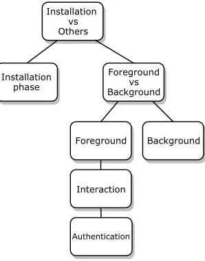
In our classification problem we have multiple classes. There are two methods in which we can predict multiple classes. Some algorithms naturally handle multi-class classification (e.g. decision trees and neural networks) where others need to perform multiple iterations of one-class classifications (e.g. Naive Bayes) in which we separate one class from the rest. If we look at our application phases, there is a natural division between the phases in this same structure, and as such the classification of the application phases can therefore also be divided in this way. We have depicted these divisions in Figure 3.

The first distinction we can make is between installation traffic and other traffic. Installation traffic is the first application phase that stands out from the rest. It is the only application phase that is dependent on an application (the Google play store). If we are able to separate the installation traffic from the other traffic we decrease the complexity of our classificaton problem by one class. The ’other’ traffic can be further split into two groups; foreground and background traffic. This division occurs because the foreground traffic can be even further divided whereas the background traffic has no further divisions. Finally we can divide the foreground traffic into interaction and authentication traffic. These two phases are the most fine-grained phases of the foreground traffic.

Based on these divisions we performed two experiments. In the first experiment we attempted to identify whether network traffic belongs to the installation phase or to any of the other phases. This is the first step in the process. This experiment is also supported by it’s importance for our defensive monitoring use case. The second experiment looked at distinguishing foreground and background traffic, which is one step further in the tree. This classification step is useful for the usage statistics and defensive monitoring use cases. The other two phases are not covered in this work, and are suggested for future work.

IV. EXPERIMENTALEVALUATION

In this section we present the experiments settings and the results of the tests we performed. We perform two experiments as explained in Section III-F. The experiments are both evaluated on our qualitative and quantitative datasets where we apply two different techniques of splitting data into a training and test set in order to achieve the best possible evaluation. We first discuss the dataset on which we evaluate our approach and then elaborate on our method of splitting data into a training and testing set.

A. Datasets

The device we used to generate the network data for our datasets was a Samsung Galaxy Note 4 running the latest Android version avaiable for that device, which was 6.0.1. In total we have captured two datasets for our experiments. One dataset contains many applications (we will refer to this as the quantitative dataset), but with smaller amounts of data for each application. We also captured one dataset with a lower amount of applications, but with larger amounts of data for

Installation vs Others

Installation phase

Foreground vs Background

Foreground Background

Interaction

Authentication

Fig. 3. Division of classification steps. The first step divides the network traffic into installation traffic or ’others’. The second step divides network traffic into foreground and background traffic. Finally the foreground traffic can be separated into interaction and subsequently authentication. We performed experiments for the first two steps.

each application (which we will refer to as the qualitative dataset). The rationale behind the quantitative dataset is that we would like to test how well our method works for a broad range of applications. However we also expect that our system will improve when larger amounts of data are available. Therefore we have captured our qualitative dataset. All the applications used in the captures originate from the top 400 most popular applications as of March 29th 2019. Some applications were left out because they were not compatible with the Android version that our test device was running, and some applications were removed from the Android play store during the experiment. This has resulted in a total of 361 applications for the quantitative dataset and 65 applications for the qualitative dataset. The full list of applications used in each dataset is listed in the Appendix.

For the quantitative dataset each application received a total of 4.000 actions, which were simulated in two iterations using the Android monkeys. The actions consisted of random taps and swipes and were constrained to stay within the specified application (e.g. a random action which would launch a different application is not possible). A delay of 100ms between different types of actions were introduced to allow the application to respond to the input it has received. In the first iteration we did an initial launch of the application and sent 2.000 random actions. A seed of 42 was used to allow for reproducibility. We then simulated activation of the home button, which sent the application into the background. The device was left idle on the home screen for 30 seconds before proceeding to the next iteration. In the second iteration the application was resumed from the background and another 2.000 actions were simulated, this time with a seed of 69.

initiated with a launch of the application, followed by a total of 3.600 actions. After the touch events from the Android monkeys the application was sent to the background by simulating activation of the home button. The device was left idle for 2 minutes on the home screen. The next iterations consisted of resuming the application from the background, simulating another 3.600 actions and finally sending the application into the background again.

Some applications require a user to authenticate before the application’s intended functionality can be accessed. Because the Android monkeys perform random touch events, the chance of obtaining such authentication data is practically nonexistent. Therefore to introduce authentication phase data in our network traffic we manually created user accounts for a subset of applications. We perform the login actions by executing a script that sends specific touch events to the device which simulates a user logging in. After the login procedure is completed we execute the same routine as with every other application. We have also indicated for which applications a login script was made in the Appendix.

B. Train Test Split

In machine learning we train a classifier on one set of data, and evaluate it on a different set of test data. Usually a large initial set of data is split into two parts, which are then used for training and testing. Standard practice is to use a (k-fold) random split which decreases the chance of having a model which coincidentally fits very well on the specific test set, but which is not generaliseable to new data. We evaluate our models by choosing a training and test set based on this method of splitting. However, recent work [28] has suggested that randomly splitting positively biases your model when predicting temporally sequential data. The reason for this is that when randomly splitting, the training set could contain datapoints from the future, which can hold valuable information when predicting datapoints of the past. Their work suggests to enforce a constraint in which all datapoints in the training set are chronologically before all datapoints in the test set to prevent any temporal bias. In order to evaluate our models as completely as possible, we have evaluated our algorithms using this method of splitting data as well.

For some applications, we were not able to obtain a valid training and test set by splitting chronologically. A valid training and test set contains network traffic of both classes. The reason that we are not able to obtain a valid split is that there are some applications with very little background traffic. Therefore if we encountered an application for which we were not able to obtain a valid train and test split, we skipped it. We have indicated the applications for which we were able to get a valid split in the Appendix.

C. Evaluation metrics

There are several different metrics that can be used to evaluate the effectiveness of a classification algorithm. These metrics are based on four different outcomes for a prediction. A true positive (TP) is defined as a prediction where the model

correctly predicts the positive class. A true negative (TN) is the correct prediction of a negative class. Similarly a false positive (FP) is a prediction where the sample belongs to the negative class and the model predicted a positive class. Finally the false negative (FN) is a sample that belongs to the positive class and the model predicted the negative class. What is considered as the positive class depends on the definition. For our experiments we use the following definitions. In the first experiment installation traffic is defined as the positive class, and other traffic is the negative class. For the second experiment, foreground traffic is considered the positive class and background traffic the negative class. We use the following metrics:

Accuracy— Accuracy is defined as the fraction of correctly predicted samples of all samples. A high accuracy means that the system is able to generally classify the samples correctly. We calculated this using the following formula:

Accuracy= T P +T N

T P+F P +T N+F N (4)

Precision— Precision is defined as the fraction of correctly identified positive samples of all positive predicted samples. A high precision means that the system is able to detect positives with a low false positive rate. We calculated this using the following formula:

Precision= T P

T P +F P (5)

Recall — Recall is defined as the fraction of identified positive samples out of all positive samples. A high recall means that the system is able to detect the majority of all positive samples. We calculated this using the following formula:

Recall= T P

T P +F N (6)

F1-score— The F1-score is a weighted combination of the recall and precision score. This score says something about the balance between precision and recall and is often used when both a low false positive rate and a high true positive rate are neccessary. This is calculated as follows:

F1-Score= 2_⇤ precision⇤recall

precision+recall (7)

D. Installation phase

We set the size of the rolling window to 1 second for this experiment (e.g. if we have a datapoint with a times-tamp of 11:04:36.435 all datapoints within [11:04:35.935 – 11:04:36.935] are included). We started by training a decision tree to classify our network traffic. We split our data into a training and test set by dividing the data in half chronologically. Afterwards we reviewed the most important features by calculating the gini importance. This metric is defined as the sum of the total decrease in node impurity, weighted by the probability of reaching that node. The probability of reaching a node is approximated by the proportion of samples that reach that specific node.

The most important feature was the DNS records. Specifically DNS records pointing to a SN encoded subdomain of gvt1.com. This domain is owned and used by google for application updating purposes3_{. This is an indicator that network traffic}

from this domain belongs to some sort of installation process. The sum of bytes received by the device was also an important feature. The tree set the threshold on 3.2 million bytes received by the device with a low average of bytes sent by the client. This is indicating that the device was downloading a large amount of data with little client activity. The unique count of flows supported this finding. Sequences where less than 5.5 unique destinations were contacted were also indicative of installation traffic. The combination of these thresholds and features, correspond to samples where a large amount of network traffic originate from a small number of google domains while the client performs little activity.

We performed classification of the network traffic using the algorithms explained in section III. The results are listed in Table II.

The Naive Bayes method scored the least of the four algo-rithms when looking at the overal metrics. The results improved when splitting randomly over splitting in chronological order for both the quantitative and qualitative captures. This is expected as the distribution is more representative of the whole distribution when we sample datapoints uniformly.

The decision tree and random forest were the best performing overall algorithms. We see a notable difference between random split training and chronological split training. This is expected as random splitting positively biases the algorithm. The algorithms achieves a higher precision than recall indicating it minimizes false positives over false negatives for the quantitative dataset. For the qualitative dataset we see a higher recall compared to precision. This is due to the fact that there is a different distribution of installation traffic compared to ‘other’ traffic for both datasets. The quantitative dataset contains a larger portion of installation traffic whereas the qualitative dataset is more skewed towards ‘other’ traffic. When the positive class is the majority it is easier to minimize false positives. Similarly when the positive class is the minority false negatives are easier to minimize. Overall the algorithms achieve a balance between the precision and recall which is

3_{https://www.systemtek.co.uk/2017/08/what-is-gvt1-com/, Accessed}

13-08-2019

what we aim for in the installation prediction problem. We do not expect the installation of new applications to be the most frequent event in a system. If it does occur, we want to be sure to detect it, but we do not want a large amount of false positives. We achieved a high accuracy and F1-score with both the decision tree and random forest. The random forest achieved a slightly higher precision compared to the decision tree and is therefore the best performing algorithm.

For a neural network with LSTM cells we needed to keep the sequential order of our data aligned when feeding the data into the network. Therefore, we could not use the random split, and only evaluated this model using the chronological split. For the neural network with LSTM cells we created an architecture which enforces a 10-step memory. This means that every iteration in the model is able to utilize data from the previous 10 samples. In order to work with the LSTM the data was reshaped into a matrix of samples where each sample consists of 10 adjacent datapoints. These are then sequentially input into the model.

The LSTM performed the worst of all the algorithms. A possible cause is that the model suffers from the imbalance in the dataset as neural networks generally need more training data compared to other models. For some applications there is a very large difference in amount of traffic for installation and others.

E. Foreground vs. Background

In this experiment we address the classification of foreground and background traffic, which is the second step in our classification tree. Foreground and background traffic has many different use cases as described in Section I. We excluded any traffic from the dataset that does not belong to the foreground or background class. Here traffic from the interaction and authentication class are considered to be a subset of foreground traffic. Therefore we mapped the labels from these two classes to the foreground class.

For this experiment we require knowledge about the appli-cation that generated the network traffic inbeforehand because the models are not yet able to classify the behaviour of the applications as a single group (e.g. there is a large difference in behaviour between a barcode scanner and a video streaming application). There are several options on how to determine which application generated the traffic, e.g. using an application identification classifier such as [7]. However, application identification using a classification method is out of scope for this work. We solved this by determining this information during the data capture process as described in Section III. After separating the network data by application, we looked at four different classifiers and evaluated their effectiveness. The classification performance was averaged over the applications and is listed per algorithm in Table III.

Naive Bayes method performed better for the qualitative captures compared to the quantitative captures when splitting chronologically. We believe this is due to the fact that the model is able to take advantage of the extra information in the qualitative captures. Compared to the other algorithms Naive Bayes method scored similarly on recall but performed worse on the precision. This can be explained by the fact that the Naive Bayes method has a preference to predict the majority class and therefore obtains a better recall, but lacks in precision.

2) Decision Tree: The second algorithm showed a large improvement over the Naive Bayes method. For the decision tree we assigned a max depth of 15, and the splitting criterion used was the gini index. We added the max depth in order to keep the model relatively small and decrease the learning time of the models. The decision tree scored best out the four algorithms when splitting in chronological order. The model came in second place when splitting randomly for the quantitative dataset. However for the qualitative dataset the random forest model was able to surpass the decision tree by a small amount. We believe there is not enough data in the quantitative dataset to develop a very complex model, which is why the decision tree outperformed the random forest. This also explains why the decision tree performed less than the random forest in the qualitative dataset. The dataset is a bit skewed towards the foreground class where we have between 2.5 and 3 times as much foreground traffic. Because the decision tree scores higher on the precision, we believe that the model is able to actually distinguish between the two classes, instead of defaulting to the majority class as in the Naive Bayes method.

3) Random Forest: After using the decision tree classifier we also learned a random forest. For this algorithm we also defined a max depth of 15 for the random forest model in order to decrease the learning time. The random forest was the best performing algorithm out of all four on accuracy, precision and recall (except for a chronological split on quantitative captures). In comparison to the Decision Tree, the accuracy and precision showed a large improvement, where the recall only showed minor improvements. This means that the ensemble trees are able to decrease the false positives where the true positives and false negatives stay relatively the same. The model performed significantly better on the random split compared to the chronological split for all metrics.

4) RNN with LSTM: The neural network performed compa-rably with the Naive Bayes method based on accuracy. However, the precision and recall are much lower compared to the other algorithms. This can be explained by the fact that the RNN mainly predicts the majority class possibly caused by the fact that there is a class imbalance. This is also reflected in the higher recall compared to the precision for the RNN model as the recall is dependent on the number of false negatives.

V. DISCUSSION

In this section, we dicuss the interpretation of our findings. We first provide some interesting notions about the algorithms in combination with our use cases. Afterwards we compare

TABLE II

CLASSIFICATION PERFORMANCE FOR THE MODEL USED IN THE INSTALLATION TRAFFIC EXPERIMENT

Accuracy Precision Recall F-measur

e

Quantitati

ve

captur

es

Randomly split

NB 0.79 0.77 0.70 0.70

DT 0.99 0.99 0.99 0.99

RF 0.99 0.99 0.99 0.99

LSTM - - -

-Chronological split

NB 0.76 0.74 0.65 0.66

DT 0.82 0.83 0.73 0.75

RF 0.85 0.86 0.72 0.79

LSTM 0.78 0.75 0.70 0.71

Qualitati

ve

captur

es

Random split

NB 0.86 0.87 0.84 0.83

DT 1.00 1.00 1.00 1.00

RF 1.00 1.00 1.00 1.00

LSTM - - -

-Chronological split

NB 0.78 0.57 0.68 0.56

DT 0.96 0.90 0.93 0.92

RF 0.96 0.92 0.93 0.93

LSTM 0.88 0.79 0.68 0.71

TABLE III

CLASSIFICATION PERFORMANCE FOR THE MODELS USED IN THE BACKGROUND AND FOREGROUND EXPERIMENT

Accuracy Precision Recall F-measur

e

Quantitati

ve

captur

es Randomly splitNB 0.83 0.68 0.77 0.66

DT 0.91 0.81 0.80 0.77

RF 0.93 0.85 0.80 0.78

LSTM - - -

-Chronological split

NB 0.61 0.48 0.52 0.45

DT 0.70 0.62 0.54 0.49

RF 0.69 0.62 0.52 0.47

LSTM 0.63 0.33 0.46 0.36

Qualitati

ve

captur

es Random splitNB 0.80 0.61 0.65 0.57

DT 0.92 0.80 0.79 0.78

RF 0.93 0.84 0.79 0.79

LSTM - - -

-Chronological split

NB 0.73 0.54 0.57 0.51

DT 0.83 0.71 0.61 0.60

RF 0.84 0.74 0.61 0.60

our work with previous work and then highlight the limitations and suggest solutions for future work.

A. Findings

This section outlines the findings from our research. We start with the algorithm choices for each use case and then we elaborate on the effect of chronological splitting the dataset in train and test. Finally we explain which method of splitting data is more realistic and touch upon methods in which an actor could evade our monitoring method.

1) Algorithm Choice: We have previously outlined two different use cases for why we are interested in mobile application phases. There are many more use cases, and each of these have different metrics that are important. The models we used in our experiments score differently on these metrics and therefore we advise to choose the model based on the metric that is important to the problem.

The Naive Bayes method and the RNN with LSTM cells scored the lowest of all models, and favor predicting the majority class in general. Because the accuracy and reliability were rather low, we believe that these methods are not sufficient to solve the problems outlined in this work. A possible solution to improve these models is to decrease the class imbalance through sampling.

The decision tree scored high on the accuracy and recall score. The model requires a low time to complete training and has a high explainability factor. Therefore if the use case requires a quick model where a high true positive rate is desired, the decision tree is a very good option.

When precision is more important, we advise to use a random forest. This model requires more training time and is less comprehensible, but achieves a higher precision and comparable or slightly higher recall than the decision tree. It also performed the best in the experiments we performed.

The evolutionary intrusion detection system requires a high accuracy and precision because false positives are one of the main problems in these systems. Therefore this use case requires a system with a high precision and accuracy. The random forest showed the best results on these fronts as it achieved a high accuracy, recall and precision. Usage statistics have a less strict requirement for a low amount of false positives, as it’s decisions are based on statistics of large amounts of datapoints and not individual events. Therefore this use case mainly focuses on accuracy and the F1-score. When training time and storage are not a problem a random forest can be used, however the decision tree scored nearly as high as the random forest on the F1-score.

2) Chronological Split: The models used in our experiments improved significantly with the qualitative dataset compared to the quantitative datasets when splitting in chronological order. We believe this is due to the fact that we observe a larger amount of events at the beginning of the qualitative dataset which are then repeated later on in this dataset, whereas in the quantitative dataset, we observe more new events later on in the dataset. This means that our model is not (yet) optimized for these smaller training phases, and therefore is less accurate

in predicting these events. This highlights the need for a model that is able to handle smaller amounts of data and able to adapt to new data and future changes as it can significantly improve classification performance.

In our opinion, the chronological split is more realistic compared to a random split, because the random split essentially introduces datapoints from the future to the training set. This is especially useful in the case for dynamic environments as with mobile applications. We often see new datapoints, and this factor should be taken into account during training. In order to get a realistic expectation of how the model can perform, a chronological split should be used. The random forest showed the most promise when trained on the chronological training set.

3) Evading the system: Evading monitoring detection is a very important aspect for adversaries. Our system is based on statistical properties of packet lengths. This makes our system vulnerable to evasion through the introduction of noise by obfuscation of packet lengths. Attackers could use a method as described by Chaddad et al. [21].

B. Comparison With Other Works

To the best of our knowledge we are the first to attempt to classify mobile application phases and therefore there is no direct related work we can compare our method with. However if we look at mobile application phases and what they consist of, we can identify two main components. You can view application phases as the resulting behaviour state for applications after some type of user action are performed. E.g. the user action ‘send email’, is done in the ‘foreground’ phase for that specific application. Therefore the two fields with which we compare our work follows directly from these components.

The first field we compare our work with is user action identification and it is the most similar to our work. User actions are usually specific to a certain application. This means that they are generally not applicable to other applications. Our mobile application phases are application agnostic and therefore can be generalised over the entire mobile application landscape. This generalisation from user actions to application phases does decrease the granularity of the output information and for some use cases a different method is better suited than ours, especially when detailed user information is crucial (e.g. user profiling or user action-based IDS). Another benefit of application phases compared to user actions is that even though we use a supervised learning classifier, new phases are much less likely to be introduced in comparison to user actions. In terms of classification performance Conti et al. [8] achieves slightly better results to that of ours. Their method classifies user actions for seven different applications and achieves accuracy and F1-score between 90 and 100%.

The second similar group are application identification methods. Both fields rely on the identification of network traffic. Mobile application identification methods usually rely on flow based prediction, such as in Taylor et al. [7]. They created AppScanner which identifies mobile applications based on a set of fingerprints created from encrypted network traffic. Their fingerprints are based on statistical features of aggregated flows. We have shown that such flow-based methods are not very effective in classifying mobile application phases. Their work achieves an accuracy between 77% and 96% when predicting applications.

C. Limitations

The main limitation of our work is lack of realistic network data. The network traffic used for this experiment was generated using random interactions by Android monkeys, performed in a in a predictable manner. We always performed a set of actions, then paused for a pre-determined amount of time, and resumed. Another factor concerning the realism of the network data is caused by the randomness in the interactions. Because they are generated randomly they may not fully resemble human-like interaction. E.g. some applications also require interactions in a specific sequence or external factors, in order to execute their inteded functionality. A barcode scanner requires barcodes to execute its functionality, and messaging apps require a second actor to interact with.

One of the features that we use for our classification is based on the DNS records. The DNS records may change, or we could see a completely new DNS record. If we have no prior knowledge to which class these changed or new records belong we cannot use the information to classify. Therefore any new DNS record that was not present in the training of the model, will be futile. In a real world setting we may have no access to the DNS records. In such case, we could perform a reverse DNS lookup to obtain the record.

D. Future Work

More realistic data could be gathered by using less pre-dictable sequences. For example we could replace the pause inbetween two interaction sequences to a random amount to introduce long and short background sequences. We could also group applications based on how they are used in real life. For example, if you look at how messaging applications are used in comparison to games, we expect to see a different use pattern. Messaging applications are used for a short time, then moved to the background. This process repeats very often. Games on the other hand, are most likely to be used for a longer period, and then moved to the background for a longer period as well. This information could be incorporated into the system.

Realistic authentication data is very hard to obtain, because most people only login once every so often, and stay logged in. Therefore to obtain realistic data for this application phase many different users are required.

A possible solution for the small amount of labeled data is to use an idea by D. Mocanu and E. Mocanu [29]. Their idea involves one-shot or few-shot learning to decrease the need

for a large amount of labeled training samples. They learn a mixture model of variational auto-encoders which automatically incorporates new predicted data samples after an initial learning period, and then re-trains the model using the new datapoints. This would allow the system to develop over time and only needs a small initial training phase.

We were not able to identify interaction and authentication traffic in our work. The main problem is that we have very little interaction and authentication data which makes it incredibly hard to learn patterns from this data. In relation to the previous statement on how to improve the realism of the dataset we also advise to look at the possibility of incorporating more interaction and authentication data. For example data which includes people chatting via a messaging application would introduce a lot of interaction traffic. Another option could be using something like a text-processing application (e.g. notes or email) as these applications also use the keyboard.

Finally one of the problems we still face is that we need to learn a model for each application, as there is a difference in network behaviour between (some) applications. The application phases are application agnostic, but the model is in it’s current state not yet able to classify the network traffic using just a single model. In order to create a robust and easy to understand system, we would like to limit the amount of models used, by grouping similar applications together. Therefore one of the ideas we have is the combination of a clustering method that groups applications into several clusters of similar applications and then use a supervised method to learn a model for each of those groups. This would allow the system to classify completely unknown applications as well, by first identifying the cluster it is most similar to, and then classifying it’s traffic with the model that belongs to that cluster.

VI. RELATEDWORK

Mobile application phase detection is a new area of research. There are some related fields, for which we will highlight the most important work in this section. Similar works can be divided into two main groups. Application identification is an area of research in which the goal is to identify which application has generated observed network traffic. The second group consists of works that try to identify specific user actions. User actions range from identifying the act of reading a twitter message to browsing through instagram photos and listening to music. We will discuss some of the most important related works for each of these categories.

A. Application identification