http://go.warwick.ac.uk/lib-publications
Original citation:
Dziuk, Gerhard and Elliott, Charles M.. (2013) Finite element methods for surface PDEs. Acta Numerica, Vol.22 . pp. 289-396.
Permanent WRAP url:
http://wrap.warwick.ac.uk/53966
Copyright and reuse:
The Warwick Research Archive Portal (WRAP) makes the work of researchers of the University of Warwick available open access under the following conditions. Copyright © and all moral rights to the version of the paper presented here belong to the individual author(s) and/or other copyright owners. To the extent reasonable and practicable the material made available in WRAP has been checked for eligibility before being made available.
Copies of full items can be used for personal research or study, educational, or not-for-profit purposes without prior permission or charge. Provided that the authors, title and full bibliographic details are credited, a hyperlink and/or URL is given for the original metadata page and the content is not changed in any way.
Publisher’s statement:
© Acta Numerica and Cambridge University Press. http://dx.doi.org/10.1017/S0962492913000056
A note on versions:
The version presented in WRAP is the published version or, version of record, and may be cited as it appears here.
http://journals.cambridge.org/ANU
Additional services for
Acta Numerica:
Email alerts: Click here
Subscriptions: Click here
Commercial reprints: Click here
Terms of use : Click here
Finite element methods for surface PDEs
Gerhard Dziuk and Charles M. Elliott
Acta Numerica / Volume 22 / May 2013, pp 289 396
DOI: 10.1017/S0962492913000056, Published online: 02 April 2013
Link to this article: http://journals.cambridge.org/abstract_S0962492913000056
How to cite this article:
Gerhard Dziuk and Charles M. Elliott (2013). Finite element methods for surface PDEs. Acta Numerica, 22, pp 289396 doi:10.1017/S0962492913000056
Request Permissions : Click here
doi:10.1017/S0962492913000056 Printed in the United Kingdom
Finite element methods for surface PDEs
∗Gerhard Dziuk
Abteilung f¨ur Angewandte Mathematik, Albert-Ludwigs-Universit¨at Freiburg im Breisgau,
Hermann-Herder-Straße 10, D–79104 Freiburg im Breisgau, Germany
E-mail: [email protected]
Charles M. Elliott
Mathematics Institute, University of Warwick, Coventry CV4 7AL, UK E-mail: [email protected]
In this article we consider finite element methods for approximating the so-lution of partial differential equations on surfaces. We focus on surface finite elements on triangulated surfaces, implicit surface methods using level set de-scriptions of the surface, unfitted finite element methods and diffuse interface methods. In order to formulate the methods we present the necessary geomet-ric analysis and, in the context of evolving surfaces, the necessary transport formulae. A wide variety of equations and applications are covered. Some ideas of the numerical analysis are presented along with illustrative numerical examples.
CONTENTS
1 Introduction 290
2 Parametrized surfaces and hypersurfaces 291 3 Partial differential equations on surfaces 301
4 Triangulated surfaces 305
5 Partial differential equations on moving surfaces 323
6 More surface PDEs 343
7 PDEs on implicit surfaces 351
8 Implicit surface finite element method 363 9 Unfitted bulk finite element method 368
10 Applications 382
References 391
1. Introduction
Surface partial differential equations arise in a wide variety of applications. Further, they are examples of partial differential equations on manifolds. As such they provide a remaining challenge within the general subject of the numerical analysis of partial differential equations. The framework is essen-tially geometric because the domain in which the equation holds is curved. They are linked naturally to the geometric equations for surfaces such as the minimal surface equation, motion by mean curvature and Willmore flow. In an earlier Acta Numerica article (Deckelnick, Dziuk and Elliott 2005) we surveyed numerical methods for geometric partial differential equations and mean curvature flow.
The purpose of this article is to give an account of numerical methods for surface partial differential equations. Our interest and research in this field was stimulated in 2003 during the Isaac Newton Institute programme ‘Computational challenges in partial differential equations’. Since this time there has been burgeoning interest in both the numerical analysis of such problems and the application to complex physical models.
The starting point was the use of surface finite elements to compute solu-tions to the Poisson problem for the Laplace–Beltrami operator on a curved surface proposed and analysed in Dziuk (1988). Here an important con-cept is the use of triangulated surfaces on which finite element spaces are constructed and then used in variational formulations of surface PDEs us-ing surface gradients. This approach was extended by Dziuk and Elliott (2007b) to parabolic (including nonlinear and higher-order) equations on stationary surfaces. The evolving surface finite element method (ESFEM) was introduced by Dziuk and Elliott (2007a) in order to treat conservation laws on moving surfaces. The key idea is to use the Leibniz (or transport) formula for the time derivative of integrals over moving surfaces in order to derive weak and variational formulations. An interesting upshot is that the velocity and mean curvature of the surface which appear in certain for-mulations of the partial differential equation do not appear explicitly in variational formulations. This gives a tremendous advantage to numerical methods that exploit this, such as those of Dziuk and Elliott (2007a, 2010). Further numerical analysis of surface finite element methods may be found in Dziuk and Elliott (2012, 2013) and Dziuk, Lubich and Mansour (2012). Applications to complex physical and biological models may be found in Eilks and Elliott (2008), Elliott and Stinner (2010), Barreira, Elliott and Madzvamuse (2011) and Elliott, Stinner and Venkataraman (2012).
Another approach is to use implicit surface methods. The starting point for these methods is the level set method for evolving surfaces (Sethian 1999, Osher and Fedkiw 2003). Here the idea is to use a level set function
the surface equation on all level sets of φ. Such methods are formulated in Bertalm´ıo, Cheng, Osher and Sapiro (2001), Greer, Bertozzi and Sapiro (2006), Burger (2009) and Dziuk and Elliott (2008, 2010).
Further, we describe in some detail numerical schemes based on the use of diffuse interfaces. These arise in phase field approximations of interface problems (Caginalp 1989, Deckelnick et al. 2005), and it is natural to ex-ploit the methodology to generate methods for solving partial differential equations on the interfaces (R¨atz and Voigt 2006, Elliott, Stinner, Styles and Welford 2011).
An important feature of the methods described in this article is the avoid-ance ofchartsboth in the problem formulation and the numerical methods. The surface finite element method is based simply on triangulated surfaces and requires the geometry solely through knowledge of the vertices of the triangulation. On the other hand, the methods based on implicit surfaces require only the level set functionφ. All the geometry is then encoded inφ. The layout of the article is as follows. In Section 2 we set basic notation and concepts concerning geometric quantities, surface gradients and integra-tion by parts for parametrized surfaces, using maps X, and hypersurfaces, using level set functionsφ. Elliptic partial differential equations on surfaces are formulated in Section 3. Surface finite elements on triangulated surfaces are formulated and analysed for elliptic equations in Section 4.
Complex applications involving surfaces and interfaces frequently require the formulation and approximation of parabolic equations on moving sur-faces. In Section 5 we formulate a scalar conservation law with a diffusive flux on a moving surface and formulate the evolving surface finite element method. Of particular note is the transport theorem for moving surfaces, which is valid triangle by triangle on an evolving surface. This is exploited together with transport property of the finite element basis functions to obtain a method which does not require explicit knowledge of the curvature or velocity, merely knowledge of the triangle vertices. Some more time-dependent equations are discussed in Section 6.
Implicit surface formulations and their numerical approximations are dis-cussed in Sections 7 and 8. Methods which use finite elements in the higher-dimensional ambient space but with variational forms on surfaces or local-ized narrow bands are considered in Section 9. Finally, we briefly discuss some applications in Section 10.
2. Parametrized surfaces and hypersurfaces
We begin in Section 2.1 by recalling some facts from elementary differen-tial geometry concerning parametrized surfaces. We continue in Section 2.2 with hypersurfaces inRn+1 and the basic analysis concepts for such
hyper-surfaces. We introduce the necessary geometric concepts, for example the notion of curvature. The formula for integration by parts is proved, and we formulate the co-area formula. In Section 2.3 we introduce global coordi-nates in a neighbourhood of a hypersurface, the Fermi coordicoordi-nates. These will be quite useful for the numerical analysis of PDEs on surfaces. For theoretical reasons we will introduce the oriented distance function. For the treatment of surface PDEs the Poincar´e inequality on surfaces is central; its proof is in Section 2.4.
2.1. Parametrized surfaces
Let n ∈ N. We call Γ ⊂ Rn+1 an n-dimensional parametrized Ck-surface
(k∈N∪ {∞}) if, for every pointx0∈Γ, there exists an open setU ⊂Rn+1
withx0 ∈U, an open connected setV ⊂Rnand a mapX:V →U∩Γ with
the propertiesX∈Ck(V,Rn+1),X is bijective and rank∇X=non V. The mapXis called a localparametrizationof Γ whileX−1is called a local
chart. A collection (Xi)i∈I, Xi ∈ Ck(Vi,Rn+1) of local parametrizations
such that∪i∈IXi(Vi) = Γ is called a Ck-atlas. IfXi(Vi)∩Xj(Vj)=∅, then
the mapXi−1◦Xj by assumption is aCk-diffeomorphism.
A function f : Γ→Risk-times differentiableif all the functions f◦Xi :
Vi →Rarek-times differentiable.
Let X ∈C2(V,Rn+1) be a local parametrization of Γ, θ ∈V. We define thefirst fundamental form G(θ) = (gij(θ))i,j=1,...,n,θ∈V by
gij(θ) =
∂X ∂θi
(θ)·∂X
∂θj
(θ), i, j= 1, . . . , n.
Superscript indices denote the inversion of the matrixGso that
(gij)i,j=1,...,n =G−1,
and byg= det(G) we denote the determinant of the matrixG.
The Laplace–Beltrami operator on Γ is defined for a twice differentiable functionf : Γ→Ras follows. Let F(θ) =f(X(θ)), θ∈V. Then
(∆Γf)(X(θ)) = 1
g(θ)
n
i,j=1
∂ ∂θj
gij(θ)g(θ)∂F
∂θi
(θ)
. (2.1)
Thetangential gradientis given by
(∇Γf)(X(θ)) =
n
i,j=1
gij(θ)∂F
∂θj
(θ)∂X
∂θi
2.2. Hypersurfaces
Definition 2.1. Let k∈N∪ {∞}. Γ⊂Rn+1 is called a Ck-hypersurface if, for each pointx0 ∈Γ, there exists an open set U ⊂Rn+1 containing x
0
and a function φ ∈ Ck(U) with the property that ∇φ = 0 on Γ∩U and such that
U ∩Γ ={x∈U |φ(x) = 0}. (2.3)
The linear space
TxΓ =
τ ∈Rn+1 | ∃γ: (−, )→Rn+1 differentiable, γ((−, ))⊂Γ, γ(0) =x andγ(0) =τ
is called the tangent space to Γ at x ∈ Γ. It is easy to show that TxΓ =
[∇φ(x)]⊥, the set of all vectors that are orthogonal to∇φ(x), where φis as in (2.3). In particular,TxΓ is an n-dimensional subspace ofRn+1.
A vectorν(x)∈Rn+1is called aunit normal vectoratx∈Γ ifν(x)⊥TxΓ
and|ν(x)|= 1. In view of the above characterization of TxΓ, we then have
ν(x) = ∇φ(x)
|∇φ(x)| or ν(x) =−
∇φ(x)
|∇φ(x)|. (2.4)
A C1-hypersurface is called orientable if there exists a continuous vector fieldν: Γ→Rn+1 such thatν(x) is a unit normal vector to Γ for allx∈Γ. The connection between the parametrized surfaces of Section 2.1 and hypersurfaces is given by the following well-known little lemma.
Lemma 2.2. Assume that Γ is aCk-hypersurface inRn+1. Then for every
x ∈Γ there exists an open set U ⊂Rn+1 with x ∈ U and a parametrized
Ck-surface X : V → U ∩Γ such that X is a bijective map from V onto
U∩Γ. IfX :V →U∩Γ is a parametrizedCk-surface andθ∈V, then there is an open set ˜V ⊂V with θ∈V˜ such that X( ˜V) is a Ck-hypersurface.
This means that locally we can always work with hypersurfaces. And we may use all the definitions from Section 2.1 for hypersurfaces.
Definition 2.3. Let Γ ⊂Rn+1 be a C1-hypersurface and let f : Γ → R be differentiable atx∈Γ. We define the tangential gradient of f atx∈Γ by
∇Γf(x) =∇f(x)− ∇f(x)·ν(x)ν(x) =P(x)∇f(x),
where P(x)ij = δij −νi(x)νj(x) (i, j = 1, . . . , n+ 1). Here f is a smooth
extension off : Γ→ Rto an (n+ 1)-dimensional neighbourhood U of the surface Γ, so thatf
Γ =f. ∇denotes the gradient in R
n+1 and ν(x) is a
The Laplace–Beltrami operatorapplied to a twice differentiable function
f ∈C2(Γ) is given by
∆Γf =∇Γ· ∇Γf =
n+1
i=1
DiDif. (2.5)
See the proof of Theorem 2.10 in Section 2.3 for the construction of an extensionf. We shall use the notation (as in the above definition)
∇Γf(x) = (D1f(x), . . . , Dn+1f(x))
for the n+ 1 components of the tangential gradient. Note that ∇Γf(x)·
ν(x) = 0 and hence∇Γf(x)∈TxΓ.
Let us show that (2.1) and (2.2) are equivalent to the settings in Defi-nition 2.3. Since the tangential gradient is a tangent vector, ∇Γf ◦X = n
i=1αiXθi with certain scalars αj. We solve this equation for α1, . . . , αn
by multiplying it byXθk, to get
Fθk =∇Γf ◦X·Xθk = n
i=1
αiXθi ·Xθk = n
i=1
αigik. (2.6)
For the first equality on the left we have used the fact that, by the chain rule applied to F(θ) = f(X(θ)), we have Fθk =
n
l=1Dlf ◦XXlθk, since
Xθk is a tangent vector. From (2.6) we infer that αl =
n
k=1Fθkgkl, and
this finally gives (2.2). Now it is easy to derive (2.1).
Lemma 2.4. ∇Γf(x) only depends on the values of f on Γ∩U, where
U ⊂Rn+1 is a neighbourhood of x.
Proof. It is sufficient to show thatf ≡0 on Γ∩U implies that∇Γf(x) = 0. Choose γ : (−, ) → Rn+1 such that γ(0) = x, γ((−, )) ⊂ Γ∩U and
γ(0) =∇Γf(x). Since f(γ(t)) =f(γ(t)) = 0 for all|t|< , we have
0 =∇f(x)·γ(0) = ∇Γf(x) +∇f(x)·ν(x)ν(x)· ∇Γf(x) =|∇Γf(x)|2,
which implies the result.
We denote by C1(Γ) the set of functions f : Γ → R, which are differen-tiable at every point x ∈ Γ and for which Djf : Γ → R, j = 1, . . . , n+ 1 are continuous. Similarly one can defineCl(Γ) (l∈N) provided that Γ is a
Ck-hypersurface withk≥l.
Definition 2.5. For Γ∈C2 we define
Hij =Diνj (i, j= 1, . . . , n+ 1). (2.7)
Weingarten map. The restriction of H to the tangent space is called the Weingarten map.
Forx∈Γ the quantity
H(x) = traceH(x) =
n+1
i=1
Hii(x) (2.8)
is the mean curvature of Γ at the point x. It differs from the common definition by a factor of n. We note that the eigenvalues κ1, . . . , κn of H
(apart from the trivial eigenvalue 0 in the ν-direction) are the principal curvaturesof Γ.
Let us have a look at the most simple example. The sphere of radius
R > 0, Γ = {x ∈ Rn+1 | |x| = R}, is given by the level set function
φ(x) =|x| −R for 0<|x|<∞. We may choose
ν = ∇φ |∇φ| =
x
|x|
and get forx∈Γ
Hij(x) =Diνj(x) =Di
xj
|x|=
1
RDixj =
1
R(δij −νiνj) =
1
R
δij−
xixj
R2
.
This matrix has an eigenvalue 0 with eigenvector Rx and neigenvaluesκj =
1
R (j= 1, . . . , n). The mean curvature of Γ is then given as H = n R.
The following result concerning the exchange of tangential derivatives is easily proved.
Lemma 2.6. For Γ∈C2 and u∈C2(Γ) we have
DiDju−DjDiu= (H∇Γu)jνi−(H∇Γu)iνj. (2.9)
fori, j= 1, . . . , n+ 1.
2.3. Global coordinates
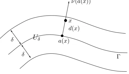
It is quite convenient to use global coordinates in a neighbourhood of a hypersurface, the so-called Fermi coordinates. This avoids working with charts and atlases (see Section 2.1) when proving results and carrying out the numerical analysis. For this one introduces theoriented distance func-tionfor Γ.
Uδ
δ δ
d(x)
(a(x))
a(x)
x ν
[image:10.493.159.373.59.183.2]Γ
Figure 2.1. StripUδ around the hypersurface Γ and normal coordinatesx=a(x) +d(x)ν(a(x)).
Assume in the following thatG⊂Rn+1is bounded and open with exterior normal ν and assume that Γ = ∂G is a Ck-hypersurface (k ≥ 2). The oriented distance function for Γ is defined by
d(x) =
infy∈Γ|x−y| x∈Rn+1\G,¯
−infy∈Γ|x−y| x∈G.
One easily verifies that d is globally Lipschitz-continuous with Lipschitz constant 1. Since∂Gis aC2-hypersurface, it satisfies both a uniform interior and a uniform exterior sphere condition, which means that for each point
x0 ∈∂Ω there are ballsB and B such that ¯
B∩(Rn+1\Ω) ={x0}, B¯∩Ω =¯ {x0},
and the radii of B, B are bounded from below by a positive constant δ
uniformly inx0. With this observation the following lemma is easily proved.
Lemma 2.8. We define
Uδ =
x∈Rn+1 | |d(x)|< δ.
Then d ∈ Ck(U
δ), and for every point x ∈ Uδ there exists a unique point
a(x)∈Γ such that
x=a(x) +d(x)ν(a(x)). (2.10)
Moreover, we have that
∇d(x) =ν(a(x)), |∇d(x)|= 1, forx∈Uδ.
We also extend the normal constantly in the normal direction: ν(x) =
ν(a(x)) for x ∈ Uδ. Thus we have introduced a global coordinate system
around Γ. Every point x ∈ Uδ can be described by its Fermi coordinates
(normal coordinates)d(x) and a(x) according to (2.10).
Theorem 2.9. Let Γ(r) ={x ∈Rn+1 | d(x) =r} be the parallel surface to Γ = Γ(0) for|r|< δ. Then
Uε
f(x) dx= ε
−ε
Γ(r)
f(x) dA(x) dr (2.11)
forf ∈C0(Uδ) and 0< ε < δ.
We note that this formula changes to
Uε
f(x) dx= ε
−ε
Γ(r)
f(x)|∇φ(x)|dA(x) dr (2.12)
if the surfaces are given by an arbitrary level set function φ as in (2.3), Γ(r) = {x ∈ Rn+1 | φ(x) = r}, and the strip around Γ is taken to be
Uδ ={x ∈Rn+1 | |φ(x)|< δ}.In this case one does not work with parallel
surfaces to Γ.
With the co-area formula one can prove the formula for integration by partson surfaces Γ.
Theorem 2.10. Assume that Γ is a hypersurface in Rn+1 with smooth boundary∂Γ and that f ∈C1(Γ). Then
Γ
∇ΓfdA=
Γ
f HνdA+
∂Γ
f µdA. (2.13)
Here,µdenotes the co-normal vector which is normal to∂Γ and tangent to Γ. A compact hypersurface Γ does not have a boundary, ∂Γ = ∅, and the last term on the right-hand side vanishes.
Note that in (2.13) dAin connection with an integral over Γ denotes the
n-dimensional surface measure, while dAin connection with an integral over
∂Γ is the (n−1)-dimensional surface measure.
Proof. We extend f to the tubular neighbourhoodUε of Γ by
f(x) =f(a(x)) (x∈Uε).
Then the chain rule gives
∂f ∂xj
(x) =
n+1
k=1
Dkf(a(x))∂ak
∂xj
(x).
The tangential derivativeDkf appears because we have that
∂ak
∂xj
(x) = ∂
∂xj
(xk−d(x)νk(x)) =δjk−νj(x)νk(x)−d(x)Hjk(x),
and the matrix (˜akj)j,k=1,...,n+1(˜akj =ak,xj) maps any vector into a tangent
vector. Thus we have
Uε
ν
µ
M(ε)
Γ
[image:12.493.140.392.63.170.2]Γ(−ε) Γ(ε)
Figure 2.2. Geometric situation around the given surface Γ. Parallel surfaces Γ(ε), Γ(−ε) and normalν, co-normalµ.
In particular, we obtain ∇f(x) = ∇Γf(x) for x ∈ Γ. We apply Gauss’s theorem tof on Uε and get
Uε
∇f(x) dx=
∂Uε
f(x)ν∂Uε(x) dA(x).
We have that∂Uε= Γ(ε)∪Γ(−ε)∪M(ε), where M(ε) ={x+rνΓ(x)|x∈
∂Γ, r∈[−ε, ε]}(see Figure 2.2). Thus
1 2ε
Uε
(I−d(x)H(x))∇Γf(a(x)) dx (2.15)
= 1 2ε
Γ(ε)
f(x)νΓ(x) dA(x)−
Γ(−ε)
f(x)νΓ(x) dA(x)
+
M(ε)
f(x)µΓ(x) dA(x)
,
with the normalνΓ and the co-normal µΓ to Γ, which do not depend onε. We take the limit ε→ 0 on both sides of this equation. Obviously, for the left-hand side
lim
ε→0
1 2ε
Uε
(I−d(x)H(x))∇Γf(a(x)) dx=
Γ
∇Γf(x) dA(x).
The limit of the first two terms of the right-hand side of (2.15) is given by
d dε
ε=0
Γ(ε)
f(x)νΓ(x) dA(x) =
Γ
f(x)H(x)νΓ(x) dA(x),
For the last term on the right-hand side of (2.15) we have that
lim
ε→0
1 2ε
M(ε)
f(x)µΓ(x) dA(x) =
∂Γ
f(x)µΓ(x) dA(x),
because the integrand does not depend onε.
The formula for integration by parts on Γ leads to the notion of a weak derivative and to the concept of Sobolev spaces on surfaces. Sobolev spaces are the natural spaces for solutions of elliptic partial differential equations. Let Γ∈C2 for the following.
Forp∈[1,∞] we letLp(Γ) denote the space of functionsf : Γ→Rwhich are measurable with respect to the surface measure dA (then-dimensional Hausdorff measure) and have finite norm, where the norm is defined by
fLp(Γ) =
Γ
|f|pdA
1
p
forp <∞, and for p=∞ we mean the essential supremum norm.
Lp(Γ) is a Banach space and for p = 2 a Hilbert space. For 1≤p < ∞
the spacesC0(Γ) andC1(Γ) are dense in Lp(Γ).
Definition 2.11. A function f ∈ L1(Γ) has the weak derivative vi =
Dif ∈ L1(Γ) (i ∈ {1, . . . , n+ 1}) if, for every function ϕ ∈ C1(Γ) with compact support{x∈Γ|ϕ(x)= 0} ⊂Γ, we have the relation
Γ
f DiϕdA=−
Γ
ϕvidA+
Γ
f ϕHνidA.
The Sobolev spaceH1,p(Γ) is defined by
H1,p(Γ) =f ∈Lp(Γ)|Dif ∈Lp(Γ), i= 1, . . . , n+ 1 with norm
fH1,p(Γ)= fpLp(Γ)+∇Γf
p Lp(Γ)
1
p.
Fork∈Nwe define
Hk,p(Γ) =f ∈Hk−1,p(Γ)|Div(k−1)∈Lp(Γ), i= 1, . . . , n+ 1,
whereH0,p(Γ) = Lp(Γ). For p = 2 we use the notation Hk(Γ) = Hk,2(Γ). We denote byv(l) allweak derivatives of order l. Then
vHk,p(Γ)=
k
l=0
v(l)pLp(Γ)
1
p .
2.4. Poincar´e’s inequality
For the convenience of the reader we show how the Poincar´e inequality for a function with mean value zero on a compactn-dimensional hypersurface can be deduced from the Poincar´e inequality in Rn+1 with the use of global coordinates.
Theorem 2.12. Assume that Γ ∈ C3 and 1 ≤ p < ∞. Then there is a constantc such that, for every function f ∈ H1,p(Γ) withΓfdA = 0, we have the inequality
fLp(Γ)≤c∇ΓfLp(Γ). (2.16)
Proof. Clearly it is sufficient to prove the inequality for L1 instead of Lp
and it is sufficient to work with smooth functions. Assume thatf ∈C1(Γ) with ΓfdA = 0. We extend this function to the tubular neighbourhood
Uδ of the surface Γ,δ being sufficiently small, by
f(x) =f(a(x)), x∈Uδ.
We state the following intermediate lemma.
Lemma 2.13. Let Γ ∈ C2 be a compact hypersurface. Then there is a constantc, such that for every 0< ε < δ we have
21εU
ε
f(x) dx−
Γ
f(x) dA(x)≤cε
Γ
|f(x)|dA(x). (2.17)
The proof of this lemma is left to the reader. We note that by the co-area formula from Theorem 2.9 we have
1 2ε
Uε
f(x) dx= 1 2ε
ε
−ε
Γ(r)
f(a(x)) dA(x) dr
with an integrand which does not depend onε.
We continue with the proof of Theorem 2.12. From (2.17) we get the inequality
(1−c1ε)
Γ
|f(x)|dA(x)≤ 1 2ε
Uε
|f(x)|dx
≤ 1
2ε
Uε
f(x)− 1 |Uε|
Uε
f(y) dydx+c2 1
|Uε|
Uε
f(y) dy
≤c3(ε)
Uε|∇
f(x)|dx+c2 1
|Uε|
Uε
by using the Poincar´e inequality forf onUε. We also have that
|U1ε|U
ε
f(x) dx= 2ε |Uε|
21εU
ε
f(x) dx−
Γ
f(x) dA(x)
≤c4ε
Γ
|f(x)|dA(x).
Thus we have the estimate
(1−c1ε−c4ε)
Γ
|f(x)|dA(x)≤c3(ε)
Uε
|∇f(x)|dx
≤c5(ε)
Γ
|∇Γf(x)|dA(x).
For the last estimate we have used that by definition ∂f∂ν = 0. A suitable choice ofε >0 gives the estimate
Γ
|f(x)|dA(x)≤c
Γ
|∇Γf(x)|dA(x).
This is Poincar´e’s inequality inL1(Γ). Forp >1 we apply this result to|f|p
instead of f, use that |∇Γ|f|p| = p|f|p−1|∇Γf| and the H¨older inequality, and the theorem is proved.
The formula for integration by parts on surfaces directly implies Green’s formula. From Theorem 2.10, using the summation convention that we sum over doubly appearing indices, we have
Γ∇Γ
f· ∇ΓgdA=
Γ
Dif DigdA=
Γ
Di(f Dig) dA−
Γ
f DiDigdA
=
Γ
f DigHνidA+
∂Γ
f DigµidA−
Γ
f∆ΓgdA.
SinceDigνi=∇Γg·ν = 0, we have the following theorem.
Theorem 2.14.
Γ
∇Γf · ∇ΓgdA=−
Γ
f∆ΓgdA+
∂Γ
f∇Γg·µdA. (2.18)
3. Partial differential equations on surfaces
3.1. Elliptic equations on hypersurfaces
The Poisson equation
We begin with the model case of the Poisson equation
−∆Γu=f (3.1)
on a compact hypersurface Γ inRn+1 and thus without boundary. Here f
is a given right-hand side or source term which is taken to be from L2(Γ) or more generally fromH−1(Γ), the dual space of H1(Γ).
Aweak solutionof (3.1) is a functionu∈H1(Γ) which satisfies the relation
Γ
∇Γu· ∇ΓϕdA=
Γ
f ϕdA (3.2)
for every test functionϕ∈H1(Γ). Sinceϕ= 1 is allowed as a test function we have to impose the condition Γf = 0 on the right-hand side. If the right-hand sidef is a functional only fromH−1(Γ), then the weak form of the equation reads
Γ∇Γ
u· ∇ΓϕdA=f, ϕ,
where the brackets stand for the evaluation of the functionalf at the func-tionϕ.
Obviously there is no uniqueness of weak solutions in this case, since every constant is a solution. We will fix the free constant by choosing the mean value ofu to vanish. The following theorem can easily be proved.
Theorem 3.1. Let Γ∈C2be a compact hypersurface inRn+1and assume
thatf ∈ H−1(Γ) with the propertyf,1= 0. Then there exists a unique solutionu∈H1(Γ) of (3.2) withΓudA= 0.
The proof is an application of the Lax–Milgram theorem or the Riesz representation theorem. The bilinear form
a(u, v) =
Γ
∇Γu· ∇ΓvdA
is a scalar product on the Hilbert space X = {u ∈ H1(Γ) | ΓudA = 0} because of Poincar´e’s inequality (2.16). The right-hand sidef was chosen to be in the spaceH−1(Γ) of linear functionals.
Besides the existence of weak solutions the most important ingredient for suitable numerics is the proof of regularity and of a priori estimates for solutions of the Poisson equation. We shall show how to prove ana priori
estimate in theH2(Γ) norm. For this we use the following little lemma, in which we use the usual notational convention for the seminorms | · |H1(Γ)
and| · |H2(Γ).
Lemma 3.2. Let Γ∈C2 and u∈H2(Γ). Then
with the constantc=
HH −2H2L∞ (Γ).
Proof. By approximation arguments we can assume that Γ ∈C3 and u∈ C3(Γ). We have
|u|2H2(Γ)=
n+1
i,j=1
Γ
(DiDju)2dA,
and with the formula for integration by parts on Γ (2.13) in combination with Lemma 2.6 we obtain (using the summation convention)
Γ
DiDjuDiDjudA=
Γ
DiDjuDjuHνi
=0
dA−
Γ
DiDiDjuDjudA
=−
Γ
Di DjDiu+Dku(νiHjk−νjHik)
DjudA
=−
Γ
DiDjDiuDjudA−
Γ
DiDku(νiHjk−νjHik)Dju
=0 dA − Γ
DkuDjuDi(νiHjk−νjHik) dA
=−
Γ
DiDjDiuDjudA−
Γ
(HH − H2)jkDjuDkudA.
For the remaining third-order term we observe that
Γ
DiDjDiuDjudA=
Γ
DjDiDiuDju+νiHjkDkDiuDjudA
=
Γ
Dj∆ΓuDjudA−
Γ
(H2)ijDiuDjudA
=−
Γ
(∆Γu)2dA−
Γ
(H2)ijDiuDjudA.
Here we have used the fact that
νiDkDiu=Dk(νiDiu)−DkνiDiu=−HikDiu.
Altogether we have shown that
|u|2H2(Γ)=∆Γu2L2(Γ)−
Γ
(HH −2H2)∇Γu· ∇ΓudA
≤ ∆Γu2L2(Γ)+HH −2H2L∞(Γ)∇Γu2L2(Γ),
and this finally proves the estimate (3.3).
Theorem 3.3. Assume that Γ∈C2 and thatf ∈L2(Γ) withΓfdA= 0. Then the weak solution from Theorem 3.1 satisfiesu∈H2(Γ) and
uH2(Γ)≤cfL2(Γ).
For the proof we use the basic estimate (choose ϕ=u in (3.2))
|u|H1(Γ)≤cfL2(Γ)
(for which we use Poincar´e’s inequality again), together with the PDE point-wise almost everywhere, to obtain
|u|H2(Γ)≤cfL2(Γ),
if the solution has square integrable second derivatives.
The H2(Γ)-regularity of u is taken from the theory of linear PDEs on Cartesian domains in Rn. Here the arguments are purely local. For this
we parametrize the C2 surface Γ according to Lemma 2.2 locally by X ∈ C2(Ω,Γ), X = X(θ) with some open domain Ω ⊂ Rn. If we set U(θ) =
u(X(θ)), thenU is a weak solution of the linear PDE
− gkjUθj√g
θk =f◦X
√
g
on Ω. For the notation see Section 2.1. The coefficients of this PDE are in
C1(Ω) and the right-hand side is inL2(Ω) because by assumption Γ∈C2. The well-known regularity result from Cartesian PDEs (see for example Gilbarg and Trudinger 1998) then gives U ∈H2(Ω) for any Ω ⊂⊂Ω, and this in turn givesu∈H2(Γ).
General elliptic PDEs
In the previous section we have shown how the Poisson equation is solved on a compact surface. The methods are easily extended to general linear elliptic PDEs in divergence form and to boundary value problems (on surfaces with a boundary):
−
n+1
i,j=1
Di(aijDju)− n+1
i=1
Di(aiu) + n+1
i=1
biDiu+cu=f − n+1
i=1
Digi. (3.4)
We assume for the given coefficients that
aij, ai, bi, c∈L∞(Γ), gi ∈L2(Γ) (i, j = 1, . . . , n+ 1).
We also assume that the coefficient vectorsa(x) = (a1(x), . . . , an+1(x)) and
g(x) = (g1(x), . . . , gn+1(x)) are tangent vectors at x ∈ Γ, that is, they
lie in TxΓ, and that the matrix A(x) = (aij(x))i,j=1,...,n+1 is symmetric
condition implies that in general constant coefficientsaij are not admissible.
They have to depend on thex-variable. Neverthelessaij =δij is obviously
allowed.
As ellipticity condition we assume a so-called Ladyzhenskaya condition, which says that there exists a numberc0 >0 such that
n+1
i,j=1
aijξiξj + n+1
i=1
aiξ0ξi+ n+1
i=1
biξiξ0+cξ02 ≥c0
n+1
i=1
ξ2i,
almost everywhere on Γ for allξ = (ξ1, . . . , ξn+1)∈Rn+1 withξ·ν= 0 and
allξ0 ∈R.
With the PDE (3.4) we associate the bilinear form a,
a(u, ϕ) =
Γ
n+1
i,j=1
aijDjuDiϕ+ n+1
i=1
aiuDiϕ+ n+1
i=1
biDiuϕ+cuϕdA,
and the functionalF,
F, ϕ=
Γ
f ϕ+
n+1
i=1
giDiϕdA,
foru, ϕ∈H1(Γ), for which we assumeF,1= 0.
Theorem 3.4. Let Γ∈C2 be a compact hypersurface. Assume that the
coefficients satisfy the above conditions. Then there exists a unique weak solution of (3.4) withΓudA= 0, that is, there exists a unique u∈H1(Γ) such that
a(u, ϕ) =F, ϕ
for everyϕ∈H1(Γ).
Proof. The proof of this theorem is a direct application of the Lax–Milgram theorem.
4. Triangulated surfaces
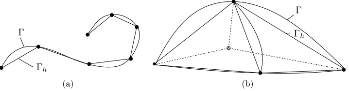
In this section we discuss the discretization of surfaces in combination with the discretization of elliptic surface PDEs. The continuous surface Γ is replaced by a piecewise polynomial surface; in the most simple case the approximating surface Γh is a polygonal one. This introduces a geometric
error between Γ and Γh, which we discuss in Section 4.2. In Section 4.4
Γ
Γh
(a)
Γ
Γh
[image:20.493.86.445.57.151.2](b)
Figure 4.1. (a) Approximation of a smooth curve by a polygonal curve and (b) approximation of a smooth surface by a polygonal surface.
4.1. Triangulations
The smoothn-dimensional surface Γ (∂Γ =∅) is approximated by a surface Γh which lies in the strip Uδ (see Lemma 2.8) and which is a Lipschitz
surface. The strip can be chosen with locally varying width: see (4.1). In particular, for n = 1, Γh is a polygonal curve, and for n = 2, it is
a triangulated (and hence polyhedral) surface consisting of triangles. A three-dimensional surface inR4 consists of tetrahedra.
We assume that the discrete triangulated surface Γh besides (4.1) has
the following properties. Γh is the union of finitely many non-degenerate
(closed)n-simplices in Rn+1. We letTh denote the set of these simplices:
Γh=
T∈Th
T.
The verticesXj(j= 1, . . . , J) of the simplices are taken to sit on the smooth
surface Γ. ForT,T˜ ∈ Th, eitherT∩T˜=∅orT∩T˜is an (n−k)-dimensional
side simplex (k∈ {1, . . . , n}) common to both of the simplicesT and ˜T. For
T ∈ Th we denote byh(T) its diameter and byρ(T) the in-ball radius. Also,
h= max
T∈Thh(T), ρ= minT∈Thρ(T).
We assume that the quantity
σ = max
T∈Thσ(T), σ(T) =
h(T)
ρ(T)
is uniformly bounded independently ofh.
Note that, by Lemma 2.8, for every simplex T ⊂ Γh there is a unique
curved simplex ˜T =a(T) ⊂ Γ. In order to avoid a global double covering (see Figure 4.2), we assume that for each point a ∈ Γ there is at most one point x ∈ Γh with a = a(x). This implies that there is a bijective
correspondence between the triangles on Γh and the induced curvilinear
Figure 4.2. Approximation of an ellipse Γ by a polygon Γh violating the simple covering condition.
[image:21.493.56.403.200.298.2](a) (b) (c) (d)
Figure 4.3. Refine and project for the sphere. We start from a
macro-triangulation (a) with 6 vertices and 8 triangles, and obtain the first (b), second (c) and sixth (d) refinement. The finest triangulation consists of 258 vertices and 512 triangles. The method of refinement is bisection of triangles.
(a) (b) (c)
Figure 4.4. Discrete spheres as a macro-triangulation ofS1,S2 andS3
[image:21.493.55.407.381.484.2]For the description of the approximation of surfaces we take the practical point of view. In order to generate triangulated parametric surfaces the two main techniques are as follows.
(1) Construct a macro-triangulation for the given smooth surface in such a way that the coarse discrete surface Γhis contained in a strip of unique
projection around Γ. Then refine and project the new nodes onto the smooth surface. For an example see Figure 4.3.
(2) Glue together patches (charts). Here one follows the classical differen-tial geometric path. The additional difficulty from the numerical point of view is the joining of two or more different grids.
Both methods can be used to generate a discretization of a standard surface such as a sphere, which can then serve as a parameter domain for the surface to be approximated. One may think of deforming the available discrete surface in order to obtain a new discrete surface. An example of this method is shown in Figure 4.5, where the surface shown is an image of a discretized cylinder.
Refine and project. The following can be understood as setting up a macro-triangulation approximating the smooth surface. For this method we use the description introduced in Section 2.3. We assume that Γ has only one connected component. We start with a discrete surface Γh contained in the
variable stripUδ,
Γh ⊂Uδ ={y+sν(y)| |s|< δ(y), y ∈Γ}, (4.1)
where for a pointy∈Γ we set
δ(y) = min
max
i=1,...,n|κi(y)|
−1
, sup
z∈Γ,z=y
L(y, z) |y−z|
with the sectional curvaturesκi. L(y, z) denotes the geodesic distance
be-tween y and z on Γ. Just as in Section 2.3, one can show that each point
x ∈ Uδ can be uniquely projected onto the smooth surface, yielding the
decomposition
x=a(x) +d(x)ν(a(x)), x∈Uδ,
witha(x) the orthogonal projection of x onto Γ and d(x) the oriented dis-tance betweenxand Γ. Given a refinement of Γh, a new refined triangulation
of Γ may be obtained by projecting the new nodes on Γh onto Γ.
For any functionη defined on the discrete surface Γh we define an
exten-sion or lift onto Γ by
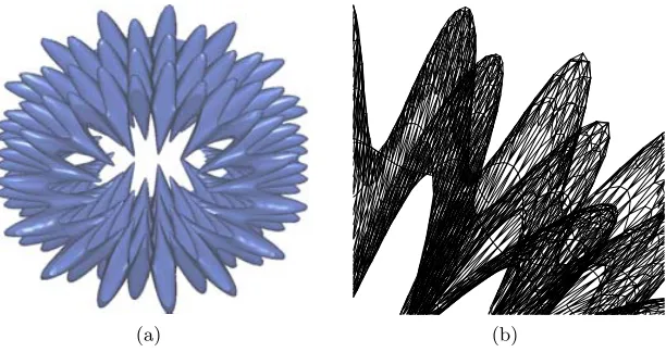
(a) (b)
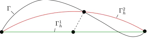
Figure 4.5. (a) A complicated hypersurface Γ approximated by a piecewise linear surface. (b) Close-up of the discrete surface Γh.
where, by our assumptions,x(a) is defined as the unique solution of
x=a+d(x)ν(a). (4.3)
Furthermore, we understand byηl(x) the constant extension from Γ in the normal directionν(a(x)).
We will use a finite element space
Sh =
φh ∈C0(Γh)|ϕh|T is linear affine for eachT ∈ Th
. (4.4)
The lifted finite element space is then
Shl =ϕh=φlh |φh ∈Sh
. (4.5)
4.2. Approximation of geometry
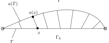
In order to avoid too many technical arguments, we begin with a piece-wise linear approximation of a smooth surface Γ ∈ C2 and its geometry. The extension to a higher-order approximation then follows the arguments in the piecewise linear case, and in fact is based upon a piecewise linear approximation.
Piecewise linear approximation of geometry
In this section we collect estimates for the geometric error which is produced by approximating the smooth surface Γ by a discrete surface Γh.
T
Γ
Γh
x
a(T)
[image:24.493.148.381.63.155.2]a(x)
Figure 4.6. A curved ‘simplex’a(T) is parametrized over a planar one. Orthogonal projection onto the smooth surface Γ.
Lemma 4.1. Assume Γ and Γh are as above. The map a : Γh → Γ is
bijective. For the oriented distance function to Γ we have the estimate
dL∞(Γh) ≤ch2. (4.6)
The quotient, δh, between the smooth and discrete surface measures dA,
and dAh, defined byδhdAh = dA, satisfies
1−δhL∞(Γh)≤ch2. (4.7)
LetP and Ph be the projections onto the tangent planes, Pij =δij−νiνj,
Ph,ij =δij−νh,iνh,j,and let
Rh=
1
δh
P(I−dH)Ph(I−dH), (4.8)
Hij =dxixj =νixj. Then
(I −Rh)PL∞(Γh)≤ch2. (4.9)
Proof. Let T ∈ Th be a simplex of the discrete surface. By assumption
it lies in the strip Uδ (see Lemma 2.8). Without loss of generality we may
assume thatT ⊂Rn× {0}. The corresponding curved triangle ˜T =a(T) is thus parametrized overT. Note that the parametrization is not given as a (vertical) graph. This is crucial for all our arguments! See Figure 4.6 for a sketch of the situation.
We let Ih denote the Lagrange interpolation on T. Since the vertices of
T lie on Γ, we have that the interpolant Ihdvanishes identically onT and,
with the well-known estimates for the Lagrangian interpolation (see Ciarlet 1978), we obtain
dL∞(T) =d−IhdL∞(T)≤ch2|d|H2,∞(T)≤ch2dC2(Uδ), (4.10)
and similarly, forj= 1, . . . , n,
To derive the estimate of the surface elements (4.7), we observe that
dA=
D12+· · ·+Dn2+1dx1· · · dxn
while dAh= dx1· · ·dxn, with
Di = (−1)n+1+i
∂a1
∂x1 · · · ∂a1
∂xn
..
. ... ...
∂ai−1 ∂x1 · · ·
∂ai−1 ∂xn ∂ai+1
∂x1 · · ·
∂ai+1
∂xn
..
. ... ...
∂an+1 ∂x1 · · ·
∂an+1 ∂xn .
Nowaj(x) =xj−d(x)νj(x), and thus forj, k= 1, . . . , n,
∂aj
∂xk
=δjk−νk(x)νj(x)−d(x)Hjk(x) =P(x)jk +O(h2), (4.12)
since from (4.10) and (4.11) we know that|νkνj| ≤ ch2 for j, k = 1, . . . , n
and|dHjk| ≤ch2. Similarly, forj = 1, . . . , n,
∂an+1
∂xj
=−νn+1νj+O(h2). (4.13)
The multilinearity of the determinant, together with (4.12) and (4.13), im-plies that fori= 1, . . . , n
Di =−νn+1νi+O(h2), Dn+1= 1 +O(h2). (4.14)
Then
D2
1+· · ·+D2n+1−1 =
D21+· · ·+Dn2+1−1
D2
1+· · ·+Dn2+1+ 1
= ν
2
n+1(1−νn2+1) +O(h2)
D2
1+· · ·+Dn2+1+ 1
=O(h2),
becauseνn2+1= 1 +O(h2). We have proved (4.7).
The proof of (4.9) follows from the previous estimates when we keep in mind that in our situationνh =en+1.Note that byνhwe mean the piecewise
constant vector defined by the normals to the simplices of Γh. We find that
(Rh−I)P =P PhP −P+O(h2) =O(h2),
since for a unit vectorz we have
|(P PhP−P)z|=|z· νh−(νh·ν)ν
because from (4.11),
|νh−(νh·ν)ν|=|en+1−νn+1ν|=
1−ν2
n+1=O(h).
This proves (4.9).
In order to compare the norms between functions on Γh and their lift
(4.2) to Γ we need the following lemma.
Lemma 4.2. Let η : Γh → R with lift ηl : Γ → R. Then, for the plane
T ⊂Γh, and smooth curved triangles ˜T ⊂Γ, the following estimates hold if
the norms exist. There is a constantc >0 independent ofh such that 1
cηL2(T)≤ η
l
L2( ˜T)≤cηL2(T), (4.15)
1
c∇ΓhηL2(T)≤ ∇Γη
l
L2( ˜T)≤c∇ΓhηL2(T), (4.16)
∇2
ΓhηL2(T)≤c∇Γ2ηlL2( ˜T)+ch∇Γη
l
L2( ˜T). (4.17)
Proof. The proof is contained in Dziuk (1988). Here we only give the main ideas. In the following let d be the distance function with respect to the smooth surface Γ. By definition (see (4.2))
η(x) =ηl(x−d(x)ν(x)), x∈Γh.
The chain rule together with the definition of the tangential gradients on smooth and discrete surface, the latter one in a piecewise sense, gives
∇Γhη(x) =Ph(x) I−d(x)H(x)
∇Γηl(a(x)), x∈Γh, (4.18)
wherePh and H are as in Lemma 4.1. The results then easily follow from
the estimates of that lemma, and in particular the estimate 0< 1c ≤δh ≤
c <∞.
For later use we list interpolation inequalities which are now available. The lemma was proved in Dziuk (1988) for the gradient. It is easily extended to theL2-estimate.
Lemma 4.3 (interpolation). For n ≤ 3 and given η ∈ H2(Γ), there
exists a uniqueIhη∈Shl such that
η−IhηL2(Γ)+h∇Γ(η−Ihη)L2(Γ)≤ch2 ∇2ΓηL2(Γ)+h∇ΓηL2(Γ)
.
(4.19)
Proof. The interpolant is constructed in an obvious way. Sinceη∈H2(Γ), by Sobolev’s embedding it is inC0(Γ) since Γ is at most three-dimensional. (Compare with Remark 4.10.) Thus the pointwise linear interpolation ˜Ihη∈
Xh is well defined. The vertices of Γh lie on the smooth surface Γ and so
the nodal values of η are well defined for this interpolation. We then lift ˜
Γ
Γ1h
[image:27.493.112.348.64.127.2]Γ2h
Figure 4.7. Higher-order approximation Γkh to Γ fork= 2.
Higher-order approximation of geometry
In the previous subsection we discussed the polygonal approximation of smooth hypersurfaces. The higher-order approximation of the smooth sur-face Γ is based on the piecewise linear approximation and is related to an isoparametric approximation to boundaries in the usual finite element methods. Let
Γ1h=
T1∈Th1
T1
be the piecewise linear approximation of Γ from the previous subsection. As shown, the map a: Γ1h → Γ is bijective. We denote by ak =Ihka∈Pk(T1)
thekth-order interpolation on the planar simplexT1 at the Lagrange nodes
ofT1. We then define the kth-order discrete surface Γkh by
Γkh=
T1∈Th1
ak(T1).
Figure 4.7 illustrates this definition. Then the next lemma follows from the proof of Lemma 4.1 in combination with the common estimates for the Lagrange interpolation on (flat) simplices: see Demlow (2009).
Lemma 4.4. Assume that Γ is as in Lemma 4.1 and let Γkh be the k th-order (k≥1) approximation described above. Then we have the estimates
dL∞(Γk
h)+1−δ
k
hL∞(Γkh)+(I−Rhk)PL∞(Γkh) ≤chk+1,
where δkh is the quotient of the surface measures on Γ and on Γkh, dA =
δk
hdAh, and δhkRkh =P(I −dH)Phk(I −dH) with the projection Phk = I −
νk
h⊗νhk onto Γkh with the normal νhk of Γkh.
4.3. Discrete charts
Let Γ be given as in Section 2.1 by local charts (Xi)i∈I, Xi ∈Ck(Vi,Rn+1).
We assume that already
Γ =
i∈I
Xi(Vih),
with Vih ⊂ Vi and triangulated domains Vih ⊂ Rn. We interpolate the
smooth parametrization Xih = IhXi, where Ih is the interpolation from
Lemma 4.3 on the polygonal domainVih. We assume that ifUij =Xih(Vih)∩
Xjh(Vjh)=∅, then the mapXih−1◦Xjh:Xjh−1(Uij)→Xih−1(Uij) is bijective,
continuous and piecewise linear. Then the discrete surface is defined by
Γh =
i∈I
Xih(Vih).
The advantage of this way to discretize the surface Γ is that it allows the approximation of immersions.
4.4. The surface finite element method(SFEM)
In the previous section we constructed and analytically treated an approx-imation of the smooth surface Γ by a discrete surface Γh. For the following
the discrete surface is the union of n-simplices, Γh =∪T∈ThT. The
exten-sion to higher-order approximations is then an extenexten-sion. For a function
g: Γh→Rwe understand thetangential gradienton the discrete surface in
the sense of Definition 2.3 as
∇Γhg=Ph∇g
in a piecewise sense, on each simplex. Here (Ph)ij = δij −νhiνhj (i, j =
1, . . . , n). ∇gdenotes the (n+ 1)-dimensional gradient of a continuation of
gorthogonal to the simplex.
In the following we will set up a finite element method on this discrete surface in order to solve PDEs. Because this approach is quite transparent, we treat piecewise linear finite elements on the discrete surface first, and we solve the Poisson equation.
We use the finite element space (see (4.4))
Sh =
φh ∈C0(Γh)|ϕh|T is linear affine for eachT ∈ Th
. (4.20)
This space is spanned by the nodal basisχ1, . . . , χJ, which is given by
χj ∈Sh, χj(Xk) =δjk (j, k= 1, . . . , J).
Here we denote byXj ∈Γ the nodes,i.e., the vertices, of the triangulation
Th. Every functionUh∈Sh has the form
Uh(x) = J
j=1
with real constantsαj (j= 1, . . . , J).
Associated with the finite element spaceSh defined on the discrete surface
is the lifted finite element space
Shl =ϕh=φlh |φh ∈Sh
. (4.21)
Note thatShl is a subspace of the continuous spaceH1(Γ). This space will appear in theoretical considerations only.
Intermediate remark. We can definerth-order finite element spaces onk th-order approximations of the smooth surface: see Lemma 4.4. The finite element space of rth order (r ≥ 1) on the piecewise linear approximation Γ1h to Γ is given by
Sh,r1 =ϕh∈C0(Γ1h)|ϕhT ∈Pr(T), T ∈ Th1
.
The general isoparametric finite element space on Γkh is then defined by
Sh,rk =ϕh∈C0(Γhk)|ϕh◦ak ∈Sh,r1
.
In the following we will continue to work with piecewise linear finite elements on piecewise linear approximations Γh = Γ1h and Sh = Sh,11 with Sh from
(4.4), to keep the methods transparent. For more information concerning the higher-order case we refer to Demlow (2009).
Definition 4.5. LetFh ∈L2(Γh) with the property that
ΓhFhdAh= 0.
A function Uh ∈Sh is a discrete solution of the Poisson equation (3.1) on
Γh if
Γh
∇ΓhUh· ∇ΓhφhdAh =
Γh
FhφhdAh, (4.22)
for every discrete test functionφh∈Sh.
The discrete Poisson equation is a linear system for the solution Uh =
J
j=1αjχj. Equation (4.22) is equivalent to n
j=1
Skjαj =Fk (k= 1, . . . , J),
where
Skj =
Γh
∇Γhχk· ∇ΓhχjdAh (k, j= 1, . . . , J)
is the stiffness matrix and Fk =
ΓhFhχkdAh (k = 1, . . . , J) is the
right-hand side. The linear system then reads
Sα=F
First we note that, for solvability of the discrete system, we need the integral over the right-hand side Fh to vanish, because in (4.22) φh = 1
is a possible test function. According to the continuous setting the linear system is not uniquely solvable, but solvable only up to additive constants.
Lemma 4.6. Assume that the situation is as in Definition 4.5. Then there is a unique discrete solution to the Poisson equation with the property that
Γh
UhdAh= 0.
Proof. We only have to show uniqueness for a solution. For this we insert
φh =Uh as a test function into the homogeneous Poisson equation ((4.22)
with Fh = 0) and find that ∇ΓhUhL2(Γh) = 0. This implies that Uh is
constant on each simplex of the triangulation separately. SinceUh∈C0(Γh),
Uh =c∈Ron Γh. Since the integral ofUh over Γh vanishes, we have that
Uh= 0 on Γh.
With respect to the implementation of the method we mention that the method is precisely like a Euclidean method except for the fact that the nodes of the triangulation are (n+1)-dimensional. Since the stiffness matrix is assembled in a loop over all simplices and set up by calculating element stiffness matrices forT ∈ Th,
ST jk =
T
∇Γhχ
T
j · ∇Γhχ
T
k dAh (j, k= 1, . . . , n+ 1),
the method is quite simple. Note that the element stiffness matrix is a planar integral. ByχTk we denote the basis function with respect to thekth vertex ofT.
4.5. Error analysis
We begin with an estimate for the geometric error when approximating bilinear forms. The most important bilinear forms are
m(u, ϕ) =
Γ
uϕdA, a(u, ϕ) =
Γ
∇Γu· ∇ΓϕdA, (4.23)
foru, ϕ∈H1(Γ), and the discrete analogues
mh(Uh, φh) =
Γh
UhφhdAh, ah(Uh, φh) =
Γh
∇ΓhUh· ∇ΓhφhdAh,
(4.24) forUh, φh∈Sh.