Formulation and optimization of the energy based blended quasicontinuum method

http://wrap.warwick.ac.uk/

Original citation:

Luskin, M., Ortner, Christoph and Van Koten, B.. (2013) Formulation and optimization of

the energy-based blended quasicontinuum method. Computer Methods in Applied

Mechanics and Engineering, Vol.253 (No.1). pp. 160-168.

Permanent WRAP url:

http://wrap.warwick.ac.uk/48640

Copyright and reuse:

The Warwick Research Archive Portal (WRAP) makes this work of researchers of the

University of Warwick available open access under the following conditions. Copyright ©

and all moral rights to the version of the paper presented here belong to the individual

author(s) and/or other copyright owners. To the extent reasonable and practicable the

material made available in WRAP has been checked for eligibility before being made

available.

Copies of full items can be used for personal research or study, educational, or

not-for-profit purposes without prior permission or charge. Provided that the authors, title and

full bibliographic details are credited, a hyperlink and/or URL is given for the original

metadata page and the content is not changed in any way.

Publisher’s statement:

NOTICE: this is the author’s version of a work that was accepted for publication in

Computer Methods in Applied Mechanics and Engineering. Changes resulting from the

publishing process, such as peer review, editing, corrections, structural formatting, and

other quality control mechanisms may not be reflected in this document. Changes may

have been made to this work since it was submitted for publication. A definitive version

was subsequently published

Computer Methods in Applied Mechanics and Engineering,

Volume 253(1). pp.160-168.

http://dx.doi.org/10.1016/j.cma.2012.09.007

A note on versions

:

The version presented here may differ from the published version or, version of record, if

you wish to cite this item you are advised to consult the publisher’s version. Please see

the ‘permanent WRAP url’ above for details on accessing the published version and note

that access may require a subscription.

FORMULATION AND OPTIMIZATION OF THE

ENERGY-BASED BLENDED QUASICONTINUUM METHOD

M. LUSKIN, C. ORTNER, AND B. VAN KOTEN

Abstract. We formulate an energy-based atomistic-to-continuum coupling method based on blending the quasicontinuum method [14] for the simulation of crystal defects. We present optimal choices of approximation parameters (blending function and finite element grid) and confirm our analytical predic-tions in numerical tests.

1. Introduction

A major goal of materials science is to predict the macroscopic properties of materials from their microscopic structure. For this purpose, it is necessary to un-derstand the behavior of defects in these materials. We propose a computational tool, the energy-based blended quasicontinuum method (BQCE), for understand-ing defects such as cracks, dislocations, vacancies, and interstitials in crystalline materials.

Accurate modeling of the region near a defect requires the use of computationally expensive atomistic models. Such models are practical only for small problems. However, a defect may interact with a large region of the material through long-range elastic fields. Thus, accurate simulation of defects requires the use of a large computational domain; typically, the size required rules out the use of atomistic models for the entire region of interest.

Fortunately, the long-range elastic fields generated by a defect are well described by continuum models which can be efficiently computed using the finite-element method. Thus, defects can be accurately and efficiently simulated by coupled mod-els which use an atomistic model near the defect and a continuum model mod-elsewhere. We call any such model anatomistic-to-continuum coupling.

Many atomistic-to-continuum couplings have been proposed in recent years [1– 3, 8, 11, 14, 19, 21]; see [13, 22] for a survey of atomistic-to-continuum couplings and computational benchmark tests. These couplings fall into two major classes: energy-based and force-based. Energy-based couplings provide an approximation to the atomistic energy of a configuration of atoms. Force-based couplings provide a non-conservative force-field which approximates the forces on each atom under the atomistic model. Our BQCE method is an energy-based coupling. Both types of

Date: December 10, 2011.

2000Mathematics Subject Classification. 65N12, 65N15, 70C20.

Key words and phrases. atomistic models, coarse graining, atomistic-to-continuum coupling, quasicontinuum method.

ML and BVK were supported in part by DMS-0757355, DMS-0811039, the PIRE Grant OISE-0967140, the University of Minnesota Supercomputing Institute, and the Department of Energy under Award Number DE-SC0002085. CO was supported by EPSRC grant EP/H003096 “Analysis of atomistic-to-continuum coupling methods”.

couplings have intrinsic advantages; the development of energy-based couplings is especially important for finite-temperature applications since equilibrium statistical properties and transition rates can be directly approximated [5, 12].

The primary source of error for most energy-based couplings is theghost force. We say that a coupling suffers from ghost forces if it predicts non-zero forces on the atoms in a perfect lattice. Although many attempts have been made to develop an energy-based coupling free from ghost forces such couplings are currently known only for a limited range of problems [6, 18, 19, 21].

Shapeev’s method [19] applies to one and two-dimensional simple crystals with an atomistic energy based on a pair interaction model, and can be extended to 3D if a modified “continuum model” is used [20]. GR-AC was proposed in [6, 21], and has recently been implemented for a two dimensional crystal with nearest neighbor multi-body interactions in [18]. No ghost force free methods are currently known for three-dimensional crystals, for multi-lattice crystals (except in 1D [15]), or for atomistic models with general multi-body interactions. The field-based coupling of Iyer and Gavini [11] is another interesting approach; however, it is unlear at present whether it is competitive in terms of computational complexity and generality.

In our BQCE method, the ghost forces cannot be eliminated but can be con-trolled in terms of an additional approximation parameter (the blending width). BQCE applies to a wide range of problems for which no ghost force free methods are known; these problems include three-dimensional crystals with general multi-body interactions as well as multi-lattices. We believe that BQCE is an attractive method for such challenging and physically important problems.

The key feature of BQCE is ablending regionwhere the atomistic and continuum contributions to the total energy are smoothly mixed. The ghost forces of the BQCE method can be made arbitrarily small by increasing the size of this blending region. BQCE shares the idea of a blending region with the bridging domain method [3], the AtC coupling [1], and the Arlequin method [2]. By contrast, the energy-based quasicontinuum method (QCE) [14], Shapeev’s method [19], and GR-AC [6, 18, 21] exhibit an abrupt transition between the atomistic and continuum models. We call any method with a blending region ablended method, and we call the weights which mix the atomistic and continuum contributions to the energy ablending function.

Both the bridging domain method and AtC coupling are very general formula-tions, each of them incorporating BQCE and QCE as special cases. Our BQCE for-mulation provides a set of specific instructions for the successful implementation of a blended method. We identify two important practical differences between BQCE and the bridging domain and AtC coupling methods. First, the BQCE method specifies a strong coupling between the atomistic and continuum regions, whereas weak couplings based on Lagrange multipliers or the penalty method have been used in most work involving the bridging domain and AtC coupling methods. Second, in BQCE, we blend the atomistic site-energy with a continuum site-energy based on the continuum site-energy defined in some formulations of the QCE method (see Section 3). This guarantees that BQCE correctly predicts the total energy of a perfect lattice subjected to uniform strain.

predicting lattice instabilities can be reduced by increasing the size of the blending region.

More recently, we have shown similar consistency results in higher dimensions [17]. We have conjectured error estimates based on these consistency results, and we use our conjectured estimates to derive complexity estimates which bound the error of the BQCE method in terms of the number of degrees of freedom used in the simulation. We then use these complexity estimates to derive optimal approxima-tion parameters for the BQCE method [17]. Implementaapproxima-tion of BQCE requires the choice of two approximation parameters: ablending function βand a finite-element mesh T which is used to compute the continuum contribution to the energy. In Section 4.3, we give optimal choices ofβ and T for the problem of a point defect in a 2D crystal.

In the present work, we demonstrate the validity of our analysis in a computa-tional test problem in which we simulate a micro-crack in a two-dimensional crystal (see Figure 1). In Section 4, we give a precise formulation of BQCE for simple lat-tices with a general multi-body interaction model. We will present a formulation of BQCE for multi-lattice crystals in a forthcoming work [17]. In Section 4.3, we offer advice on choosing the blending functionβ and the mesh T based on our analysis in [17]. The results of this analysis are summarized in Table 4.3.

In Section 5, we describe the details of our numerical experiment. We use an atomistic energy based on the Embedded Atom Method. We did not choose our atomistic energy to model any specific physical material; instead, the atomistic energy is a toy model chosen for its simplicity. Finally, we present the results of our experiment in Section 5.3. The observed rates of convergence are in agreement with the rates predicted in Section 4.3. In particular, the error of BQCE in the W1,2

semi-norm decreases as DoF−12 _{where DoF is the number of degrees of freedom.}

2. The Atomistic Energy

Let Λ be a d-dimensional Bravais lattice. We call Λ thereference lattice, and we refer to pointsξ∈Λ asatoms. Let

Y :={y: Λ→_Rd_{;y(ξ)6=y(η) for allξ6=η}}

be the set ofdeformations of Λ. Let Ωa ⊂Λ be a finite subset of Λ. We call Ωa

theatomistic computational domain.

In the Embedded Atom Method (EAM), the energy of Ωasubjected to

deforma-tiony takes the form

(2.1) Ea_{(y) :=} X

ξ∈Ωa

X

η∈Λ

η6=ξ 1

2φ |y(η)−y(ξ)|

+G

X

η∈Λ

η6=ξ

ρ |y(η)−y(ξ)|

,

whereφis a pair potential,ρis an electron density function, andGis an embedding function. We call the inner sum

(2.2) Eξa(y) :=

X

η∈Λ

η6=ξ 1

2φ |y(η)−y(ξ)|

+G

X

η∈Λ

η6=ξ

ρ |y(η)−y(ξ)|

Λ. This is because the pair potential φand electron density functionρ are taken to have acut-off radius rc such that

φ(r) =ρ(r) = 0 for allr≥rc.

When defining the Blended Quasicontinuum Energy (BQCE), we will consider a more general class of potentials than EAM. Roughly speaking, we will require only that the total energy can be decomposed into a sum of localized site-energies associated with each atom. Bylocalized, we mean that the energy associated with an atom ξ does not depend on the positions of atoms beyond a certain cut-off distance. Such an assumption may be violated for certain energies arising from quantum mechanics, but does hold for most empirical potentials including EAM, the bond-angle potentials, and so forth. In addition, we require that the site-energies arehomogeneous; that is, the energies of atoms which have the same local environment are the same.

To make these assumptions precise, we letEa

ξ(y) denote the site-energy associated with atomξunder deformationy and require that it is of the form

(2.3) Ea

ξ(y) :=V

y(η)−y(ξ) :η∈Λ\ {ξ},|y(η)−y(ξ)| ≤rc ,

where V the site-energy potential. We assume that the resulting site-energies are twice continuously differentiable, that is, Ea

ξ ∈C

2_{(Y). The restricted dependence}

ofEa

ξ on atoms within the cut-off radius may also be expressed in the form

∂Ea

ξ

∂y(η)(y) = 0 for allη with|y(η)−y(ξ)| ≥rc.

This quantifies the requirement that the site-energy is localized. GivenEa

ξ we define the energy of Ω subjected toy by

(2.4) Ea_{(y) :=}X

ξ∈Ω

Ea

ξ(y).

We call an energy of the form (2.4) whereEa

ξ satisfies (2.3)homogeneous. When we define the Cauchy–Born strain energy density corresponding to (2.4) in Section 3, we use that Ea _{is homogeneous: if E}a _{is not homogeneous, the energy per unit}

volume in a perfect lattice subjected to uniform strain may not be well defined.

Remark 2.1. The locality assumption can, in principle, be replaced by an assump-tion that the interacassump-tion strength decays sufficiently rapidly with increasing distance between atoms.

Remark 2.2. Homogeneity of the site-energy is our main assumption that is vio-lated for multi-lattices. We show in [17] how to generalize our formulation for that scenario.

3. The Cauchy–Born Site Energy

BQCE is a coupling of an atomistic energy based on (2.4) with a coarse-grained continuum elastic energy based on the Cauchy–Born strain energy density (3.1). Let vor(ξ) denote the Voronoi cell of a site ξ∈ Λ. Then the Cauchy–Born strain energy densityW : GL(_Rd_)→

Rcorresponding to V is defined by

(3.1) W(F) := 1

|vor(0)|E

a 0(y

whereyF ∈Y is the homogeneous deformation yF(ξ) =F ξ. W(F) may be inter-preted as the energy per unit volume in Λ subjected to strain F. Note that the assumption of homogeneity (2.3) ensures thatEa

ξ(y

F_{) =E}a

0(yF) for allξ∈Λ.

We will use the Cauchy–Born strain energy density (3.1) to derive a coarse-grained continuum energy suitable for coupling with the atomistic energy (2.4). First, we define a space of coarse-grained deformations. Choose representative atoms (repatoms) in Λ, and let Λrep _{denote the set of repatoms. Let T be a}

triangulation of Λrep_{, and let P}1_{(T) denote the set of all functions y :}

Rd →Rd

that are continous and piecewise affine with respect toT. We callP1_{(T) the set of}

coarse-grained deformations. The Cauchy–Born energy of a deformationy∈P1_(T)

in a domain Ω is then given by

Ec(y) :=

Z

Ω

W(∇y(x))dx.

The Cauchy–Born approximation is analyzed, for example, in [4, 7, 10].

The definition of the QCE method [14] and our construction of the BQCE method in the next section use a Cauchy–Born site-energy Ec

ξ, which is analogous to the atomistic site-energyEa

ξ. Fory∈P

1_{(T) andξ∈Λ, we defineE}c

ξ by

Ec

ξ(y) : =

Z

vor(ξ)

W(∇y(x))dx

= X

T∈T

|vor(ξ)∩T|W(∇y|T). (3.2)

In formula (3.2),|vor(ξ)∩T|denotes the volume of the intersection of vor(ξ) with the element T. We observe that the sum on the right hand side of equation (3.2) is finite because only finitely many elementsT ∈ T can intersect vor(ξ).

4. _{The Blended Quasicontinuum Energy}

4.1. Formulation of the BQCE method. The Blended Quasicontinuum En-ergy (BQCE) is an atomistic-to-continuum coupling based on the Quasicontinuum Energy (QCE) of Tadmor et al. [14]. In QCE, the reference domain Ωa is

parti-tioned into an atomistic regionA and a continuum region C, and the QC energy EQC _:P1_(T)→

Ris defined by

(4.1) EQC_{(y) :=}X

ξ∈A Ea

ξ(y) +

X

ξ∈C Ec

ξ(y).

In BQCE, the atomistic and continuum energies per atom are weighted averages. Given a blending function β : Ωa → [0,1] the BQCE energy Eβ : P1(T) → R is

defined by

(4.2) Eβ(y) := X

ξ∈Ωa

β(ξ)Eξc(y) + (1−β(ξ))E

a

ξ(y).

The BQCE energy can be rewritten in the form

Eβ(y) = X ξ∈Ωa

β(ξ)

Z

vor(ξ)

W(∇y)dx+ (1−β(ξ))Eξa(y)

= X

ξ∈Ωa

X

T∈T

β(ξ)|vor(ξ)∩T|W(∇y|T) + X ξ∈Ωa

(1−β(ξ))Eξa(y)

= X

T∈T

v_TβW(∇y|T) + X ξ∈Ωa

(1−β(ξ))Ea

ξ(y), (4.3)

where theBQCE-effective volume of the elementT is defined by

(4.4) vβ_T := X

ξ∈Ωa

β(ξ)|vor(ξ)∩T|.

Remark 4.1. The triangulation T need not cover the entire domainΩa. ForT a

triangulation which covers only part of Rd, define

Ω(T) : =∪T∈TT, and

P1(T) : ={y: Ω(T)∪Λ→Rd: y piecewise affine w.r.t. T onΩ(T)}.

We observe that Eβ_{(y) is defined for y ∈ P}1_{(T) if for every ξ ∈ Ω}

a such that

β(ξ)>0 we have vor(ξ)⊂Ω(T). In particular, it is not necessary to assume that the triangulation T is refined to atomistic scale anywhere in the domain Ωa. It is

possible that the use of a mesh which is not refined to atomistic scale may make the implementation of BQCE easier and more efficient in some cases.

4.2. Far-field boundary conditions. A typical application of the BQCE method is the simulation of a defect or defect region in an infinite crystal. To that end, we require far-field boundary conditions at the domain boundary. We propose two choices.

4.2.1. Dirichlet boundary conditions. Let S ⊂ T be a finite subset of T, and let Ω(S) :=∪S∈SS be a polygonal domain. When Dirichlet boundary conditions are imposed, the deformation of the boundary ∂Ω(S) of Ω(S) is fixed to agree with somey0∈P1(T). Precisely, we let

(4.5) Adm :=

y∈P1(T) :y(x) =y0(x) for all x∈∂Ω(S)

denote the space of admissible deformations. We then solve the problem

(4.6) Findy∈argmin

z∈Adm

Eβ_(z),

where we interpret argmin_z∈AdmEβ_{(z) as the set oflocal minimizers ofE}β_.

4.2.2. Periodic boundary conditions. A popular method to construct artificial far-field boundary conditions is to formulate the problem in a periodic cell. To that end, suppose that Ω(T) = Rd, T is periodic, and letS ⊂ T be the finite element

mesh on one periodic cell. That is, suppose that there exists a matrixA∈GL(Rd)

such that

T = [ n∈Zd

An+S ,

Given ahomogeneous far-field macroscopic strain F ∈ GL(Rd), we then define

the admissible set as

(4.7) Adm :=

y∈P1(T) :y(x+An) =y(x) +F Anfor allx∈_Rd _.

The associated variational problem can again be stated as (4.6).

4.3. Complexity and optimal parameters. In [17], we conjecture an error es-timate for BQCE in 2D and 3D. The conjecture is based on our error analysis of BQCE in 1D [23] and on the consistency estimates for BQCE in 2D and 3D in [17]. Following [16, Sec. 7.1], we use our conjectured error estimate to derivecomplexity estimates, which are bounds on the error of the BQCE method in terms of the number of degrees of freedom. We use our complexity estimates to guide the choice of optimal approximation parametersT andβ.

Letyabe an equilibrium of the atomistic energy, and letyβbe an equilibrium of BQCE with the same boundary conditions asya. Let hbe the mesh size function

of the triangulationT (h(x) = diam(T) for a.e. x∈T), and letβ be the blending function. Then we conjecture an estimate of the form:

Err :=kDya−DyβkLp.khD2y_ak_Lp_(C)+kD2βk_Lp

=: CG + GF, (4.8)

for all p ∈ [1,∞] (however, for p ∈ {1,∞}, it is unclear in what generality this result may hold). In (4.8), D2_y

a and D2β should be interpreted as the second

derivatives of smooth interpolants ofya and β, andC := supp(β). The first term,

CG =kh∇2_y

akLp_(C), is the finite elementcoarsening error, while the second term,

GF =kD2_{βkLp, measures the effect of the ghost forces.}

We now describe the problem of a point defect in a 2D crystal. To quantify the notion of a point defect, we assume that for someα >0,

(4.9) |D2ya(x)| 'r−α, wherer=|x|.

It has been observed in numerical experiments that α= 2 for a dislocation, and that α = 3 for a vacancy [9, 16]. We assume that the reference domain Ω is a roughly circular region of radiusN atomic spacings centered at the origin. We let K0 > 0 be the radius of the atomistic region surrounding the defect, and we let

K1 > 0 be the width of the blending region. We then choose a radial blending

functionβ of the form

(4.10) β(x) :=

      

0 ifr < K0,

β0

_|x|−K

0 K1

ifK0≤r < K0+K1,

1 ifK0+K1≤r,

whereβ0: [0,1]→[0,1] is a twice continuously differentiable function withβ0(0) =

β0

0(0) =β00(1) = 0 andβ0(1) = 1.

We summarize our complexity estimates for BQCE in Table 4.3. These estimates are proved in [17]. We distinguish three cases based on the value ofγ:= _pαp₊₂. In the second column, we give the optimal rates of convergence for BQCE. The optimal rates are attained whenK1is given in terms ofK0by the formula appearing in the

third column and when the mesh size functionhis given by

(4.11) h(x) =

|x| K0

γ

Table 1. Complexity estimates and optimal approximation

pa-rameters for BQCE [17]. The estimates above are for the problem of a point defect in a two-dimensional crystal. The variables K0,

K1,N, andαare defined in Section 4.3, andγ:= _pαp₊₂. In all cases,

the optimal rate of convergence is attained whenh=_K|x| 0

γ

and whenK1is given in terms ofK0by the formula in the third column

above.

Case Complexity Estimate Optimal Parameters

γ >1 k∇ya− ∇yβkLp.DoFmax{

1

p−1,

1

p− α

2} _K1=K0

γ= 1 k∇ya− ∇yβkLp.DoFmax{

1

p−1,−12} _K1=K0ln

N K0

12

γ <1 k∇ya− ∇yβkLp.DoFmax{

1

p−1,−

1

2} _K1=Kγ

0N 1−γ

Remark 4.2. The rates of convergence depend on the geometry of the problem and on the norm in which the error is measured. We observe that the error of BQCE does not decrease withDoFwhen measured in theW1,1_{-seminorm. This is because}

the W−1,1_{-norm of the ghost force does not decrease as the size of the blending}

region increases.

Remark 4.3. When αis small, the rate of convergence of BQCE is the same as the rate of convergence of Shapeev’s method in some norms. In fact, if α ≤ 2 (e.g., a dislocation), then theW1,2_{-error of Shapeev’s method decreases as DoF}−1

2 with the number of degrees of freedom [16]. We predict the same rate of conver-gence for BQCE when α ≤ 2. On the other hand, when α is larger, a patch test consistent coupling such as Shapeev’s method may converge faster than BQCE. Whenα >2(e.g., a vacancy, micro-crack, or dislocation dipole), the W1,2_{-error of}

Shapeev’s method decreases asDoF12−

α

2, whereas theW1,2-error of BQCE decreases as DoF−12. Roughly speaking, this is because when αis small, the coarse-graining error dominates, but whenαis large, the ghost force error dominates.

5. Numerical Example

5.1. Setup of the atomistic model. In the 2D triangular lattice defined by

Λ :=

1 1/2 0 √3/2

·Z2

we choose a hexagonal domain Ωawith embedded micro-crack as described in

Fig-ure 1. The sidelength of the domain is N = 300 atomic spacings, and a “micro-crack” is introduced by removing a segment of nine atoms Λcrack_:={−4e

1, . . . ,4e1}

at the center of Ωa.

The domain is supplied with periodic boundary conditions (4.7) with macro-scopic strain given by

F:=

1 γII

0 1 +γI

·F0,

whereF0∝Iminimizes the Cauchy–Born stored energy functionW andγI, γIIare

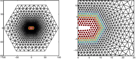
−100 −50 0 50 100 −100

−50 0 50 100

0 5 10 15 20 25

−10 −5 0 5 10

Figure 1. Deformed configuration in atomic units of a BQCE

solution for a microcrack in a computational domain with approx-imately 3N2 _{atoms (N = 100 in this figure, but N = 300 in the}

benchmark described in Section 5.3). The color and size of the atom positions indicate the value of the blending function.

the atomistic model (for the computation of errors) in the same periodic domain in order to avoid taking into account additional approximation errors due to the choice of far-field boundary condition.

The site energy is given by the EAM toy-model (2.2), with

φ(r) =η(r)

e−2a(r−1)−2e−a(r−1)

, ρ(r) =η(r)e−br, and

G( ¯ρ) =c

( ¯ρ−ρ¯0)2+ ( ¯ρ−ρ¯0)4,

where a, b, c,ρ¯0 ∈ R are parameters of the model and η ∈ C2,1(R) is a cut-off

function defined through

    

η(r) = 1, forr < rcut1 ,

η(r)∈[0,1], forrcut

1 < r < r2cut,

η(r) = 0, forr > rcut2 ,

and the requirement thatηis a quintic polynomial in [rcut

1 , r2cut], wherer1cut, r2cutare

additional parameters of the model. In our computational experiment we choose

a= 4.4, b= 3, c= 5, t0= 6e−b, rcut1 = 1.8, rcut2 = 2.5.

5.2. Setup of the BQCE method. Our implementation of the BQCE method is based on (4.3), using standard finite element assembly techniques. The construction of the blending function is governed by two approximation parameters:

• K0∈Ndenotes the number of atomic layers surrounding the micro-crack

whereβ = 1;

• K1∈Ndenotes the number of atomic layers in the blending region.

For the micro-crack problem we expect α = 3 in the context of Section 4.3. Hence, according to Table 4.3, the choiceK1:=K0 (so that the number of atoms

Letdhop(ξ, η) denote the hopping distance in the triangular lattice (with natural

extension to sets), then we define

Λa:=ξ∈Ωa:dhop(ξ,Λcrack)≤K0 , and

Λb:=

ξ∈Ωa:K0< dhop(ξ,Λcrack)≤K0+K1 .

We consider three choices of the blending function, which are all easily defined for general interface geometries:

• QCE:choosing β to be the characteristic function of the atomistic region Λa_{, andK}

1= 0, yields the QCE method defined in (4.1).

• Linear Blending: Letd(ξ) denote the hopping distance from the atomistic region, then we choose

βlin(ξ) := max(1, d(ξ)/K1).

• Smooth Blending: Let ∆2_iβ(ξ) := β(ξ+ai)−2β(ξ) +β(ξ−a1), and let

Φ(β) :=P

ξ∈Ωa

P3

i=1|∆ 2

iβ(ξ)|2, then we define

βsmooth:= argmin

Φ(β) :β(ξ) = 0 in Λaand β(ξ) = 1 in Ωa\Λa∪Λb .

The third approximation parameter is the finite element mesh in the continuum region. We coarsen the finite element mesh away from the boundary of the blending region according to the rule suggested by the complexity estimates in Table 4.3. As a matter of fact it turns out that the mesh size growth is too rapid to create shape-regular meshes, hence we also impose the restriction that neighbouring element can at most grow by a prescribed factor; this introduces an additional logarithmic factor in the complexity estimates [16, Sec. 7.1].

The resulting energy functional is minimized using the preconditioned Pol´ak– Ribi`ere conjugate gradient algorithm described in [22]. We removed the termination criterion in this algorithm and allowed it to converge to its maximal precision, that is, until the numerically computed descent direction ceases to be an actual descent direction for the energy; this occurs at an accuracy of 10−5_{to 10}−6_{in atomic units.}

5.3. Rates of Convergence. In our numerical experiment, we chooseγI =γII=

0.03 (3% shear and 3% tensile stretch), solve the BQCE problem (to be precise, the QCE and the BQCE problems for linear and smooth blending functions) for increasing parameters K0, and compute the error relative to the exact atomistic

solution.

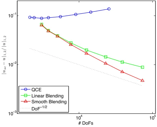
The relative errors in theW1,2_{-seminorm are displayed in Figure 2; the relative}

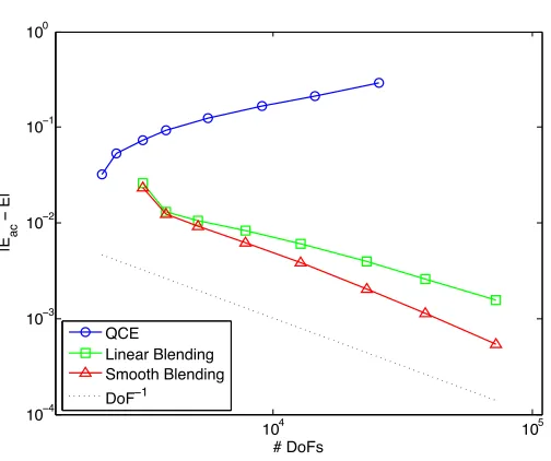
errors in theW1,∞_{-seminorm are displayed in Figure 3; the errors in the energy are} displayed in Figure 4. We observe clear qualitative agreement with our theoretical predictions.

However, it is worth pointing out that the advantage of a smooth blending func-tion is less pronounced than our theory might suggest. As a matter of fact, it appears that smooth blending functions only become advantageous for fairly wide blending regions. (The two last datapoints in the graphs for the BQCE methods correspond, respectively, toK1= 22 andK1= 32.

References

104 105

10−3

10−2

10−1

# DoFs

|

uac

−

u

|1,

2

/

|

u

|1,

2

QCE

Linear Blending Smooth Blending

DoF−1/2

Figure 2. Convergence rates in the energy-norm (the H1

-seminorm) for the micro-crack benchmark problem described in Section 5.

104 105

10−4 10−3 10−2 10−1

# DoFs

|

uac

−

u

|1,

∞

/

|

u

|1,

∞

QCE

Linear Blending Smooth Blending DoF−1

Figure 3. Convergence rates in the W1,∞-seminorm for the micro-crack benchmark problem described in Section 5.

104 105 10−4

10−3 10−2 10−1 100

# DoFs

|E ac

−

E|

QCE

Linear Blending Smooth Blending DoF−1

Figure 4. Convergence rates in the energy, for the micro-crack

benchmark problem described in Section 5.

[3] T. Belytschko and S. P. Xiao. Coupling methods for continuum model with molecular model. International Journal for Multiscale Computational Engineering, 1:115–126, 2003.

[4] X. Blanc, C. Le Bris, and P.-L. Lions. From molecular models to continuum mechanics.Arch. Ration. Mech. Anal., 164(4):341–381, 2002.

[5] L. M. Dupuy, E. B. Tadmor, F. Legoll, R. E. Miller, and W. K. Kim. Finite-temperature quasicontinuum. manuscript, 2011.

[6] W. E, J. Lu, and J. Yang. Uniform accuracy of the quasicontinuum method.Phys. Rev. B, 74(21):214115, 2006.

[7] W. E and P. Ming. Cauchy-Born rule and the stability of crystalline solids: static problems. Arch. Ration. Mech. Anal., 183(2):241–297, 2007.

[8] H. Fischmeister, H. Exner, M.-H. Poech, S. Kohlhoff, P. Gumbsch, S. Schmauder, L. S. Sigi, and R. Spiegler. Modelling fracture processes in metals and composite materials. Z. Metallkde., 80:839–846, 1989.

[9] F. C. Frank and J. H. van der Merwe. One-dimensional dislocations. I. static theory.Proc. R. Soc. London, A198:205–216, 1949.

[10] T. Hudson and C. Ortner. On the stability of bravais lattices and their cauchy–born approx-imations.M2AN Math. Model. Numer. Anal., 46, 2012.

[11] M. Iyer and V. Gavini. A field theoretical approach to the quasi-continuum method.Journal of the Mechanics and Physics of Solids, 59(8):1506 – 1535, 2011.

[12] W. K. Kim, E. B. Tadmor, M. Luskin, D. Perez, and A. Voter. Hyper-qc: An accelerated finite-temperature quasicontinuum method using hyperdynamics. manuscript, 2011. [13] R. Miller and E. Tadmor. A unified framework and performance benchmark of fourteen

multiscale atomistic/continuum coupling methods. Modelling Simul. Mater. Sci. Eng., 17, 2009.

[14] M. Ortiz, R. Phillips, and E. B. Tadmor. Quasicontinuum analysis of defects in solids. Philo-sophical Magazine A, 73(6):1529–1563, 1996.

[15] C. Ortner and A. Shapeev. work in progress.

[16] C. Ortner and A. V. Shapeev. Analysis of an Energy-based Atomistic/Continuum Coupling Approximation of a Vacancy in the 2D Triangular Lattice.ArXiv e-prints, 1104.0311, Apr. 2010.

[18] C. Ortner and L. Zhang. Construction and sharp consistency estimates for atom-istic/continuum coupling methods with general interfaces: a 2d model problem. arXiv:1110.0168.

[19] A. Shapeev. Consistent energy-based atomistic/continuum coupling for two-body potentials in one and two dimensions.Multiscale Model. Simul., 9(3):905–932, 2011.

[20] A. V. Shapeev. Consistent energy-based atomistic/continuum coupling for two-body poten-tials in three dimensions. arXiv:1108.2991.

[21] T. Shimokawa, J. Mortensen, J. Schiotz, and K. Jacobsen. Matching conditions in the qua-sicontinuum method: Removal of the error introduced at the interface between the coarse-grained and fully atomistic region.Phys. Rev. B, 69(21):214104, 2004.

[22] B. Van Koten, X. H. Li, M. Luskin, and C. Ortner. A computational and theoretical in-vestigation of the accuracy of quasicontinuum methods. In I. Graham, T. Hou, O. Lakkis, and R. Scheichl, editors, Numerical Analysis of Multiscale Problems. Springer, to appear. arXiv:1012.6031.

[23] B. Van Koten and M. Luskin. Analysis of energy-based blended quasicontinuum approxima-tions.SIAM J. Numer. Anal., to appear. arXiv:1008.2138v3.

M. Luskin, 127 Vincent Hall, 206 Church St. SE, Minneapolis, MN 55455, USA E-mail address:[email protected]

C. Ortner, Mathematics Institute, Zeeman Building, University of Warwick, Coven-try CV4 7AL, UK

E-mail address:[email protected]