warwick.ac.uk/lib-publications
Original citation:
Song, Baofang, Barkley, Dwight, Hof, Björn and Avila, Marc. (2017) Speed and structure of
turbulent fronts in pipe flow. Journal of Fluid Mechanics, 813 . pp. 1045-1059.
Permanent WRAP URL:
http://wrap.warwick.ac.uk/85635
Copyright and reuse:
The Warwick Research Archive Portal (WRAP) makes this work by researchers of the
University of Warwick available open access under the following conditions. Copyright ©
and all moral rights to the version of the paper presented here belong to the individual
author(s) and/or other copyright owners. To the extent reasonable and practicable the
material made available in WRAP has been checked for eligibility before being made
available.
Copies of full items can be used for personal research or study, educational, or not-for profit
purposes without prior permission or charge. Provided that the authors, title and full
bibliographic details are credited, a hyperlink and/or URL is given for the original metadata
page and the content is not changed in any way.
Publisher’s statement:
This article has been published in a revised form in Journal of Fluid Mechanics
http://dx.doi.org/10.1017/jfm.2017.14
This version is free to view and download for
private research and study only. Not for re-distribution, re-sale or use in derivative works. ©
copyright holder.
A note on versions:
The version presented here may differ from the published version or, version of record, if
you wish to cite this item you are advised to consult the publisher’s version. Please see the
‘permanent WRAP URL’ above for details on accessing the published version and note that
access may require a subscription
Under consideration for publication in J. Fluid Mech.
Speed and structure of turbulent fronts in
pipe flow
By Baofang Song
1,2†
, Dwight Barkley
3, Bj¨
orn Hof
4, & Marc Avila
1,21
Center of Applied Space Technology and Microgravity, University of Bremen, 28359 Bremen, Germany
2Institute of Fluid Mechanics, Friedrich-Alexander-Universit¨at Erlangen-N¨urnberg, 91058
Erlangen, Germany
3
Mathematics Institute, University of Warwick, Coventry CV4 7AL, United Kingdom
4Institute of Science and Technology Austria, 3400 Klosterneuburg, Austria
(Printed ?; revised ?; accepted ?. - To be entered by editorial office)
Using extensive direct numerical simulations, the dynamics of laminar-turbulent fronts in pipe flow is investigated for Reynolds numbers betweenRe=2000 and 5500. We here investigate the physical distinction between the fronts of weak and strong slugs both by analysing the turbulent kinetic energy budget and by comparing the downstream front motion to the advection speed of bulk turbulent structures. Our study shows that weak downstream fronts travel slower than turbulent structures in the bulk and correspond to decaying turbulence at the front. AtRe '2900 the downstream front speed becomes faster than the advection speed, marking the onset of strong fronts. In contrast to weak fronts, turbulent eddies are generated at strong fronts by feeding on the downstream laminar flow. Our study also suggests that temporal fluctuations of production and dissi-pation at the downstream laminar-turbulent front drive the dynamical switches between the two types of front observed up toRe '3200.
1. Introduction
In pipe flow, turbulence first appears at relatively low Reynolds numbers in localised patches known as puffs. Only at higher Reynolds numbers does turbulence begin to expand in streamwise extent and eventually render the flow fully turbulent. Such ex-panding turbulent regions are known as slugs. The structure of puffs and slugs, as well as the transformation process between them as Reynolds number increases, has been the subject of many experimental and numerical studies (Lindgren 1969; Wygnanski & Champagne 1973; Sreenivasan & Ramshankar 1986; Darbyshire & Mullin 1995; Durst &
¨
Unsal 2006; Nishiet al.2008; Duguetet al.2010).
In more detail, puffs are arrowhead-shaped structures with a sharp upstream front and a diffusive downstream front (see figure 1a). Within a puff, individual fluid parcels do not persist in a turbulent state. Rather turbulence is generated at the upstream front and then decays continuously as fluid parcels pass to the downstream front (Rotta 1956; Wygnanskiet al.1975; Darbyshire & Mullin 1995; van Doorne & Westerweel 2009; Hof
et al.2010). In contrast, at high Reynolds numbers slugs have a spatially extended bulk region between the upstream and downstream fronts, and in the bulk region turbulence shows no significant spatial variation, indicating that the interior part of slugs is in a
0.6 0.8 1 1.2 1.4 1.6
2000 2500 3000 3500 4000 4500 5000 5500
upstream front downstream front
Speed
Reynolds number (d)
[image:3.595.102.480.102.403.2]Nishi et al. 2008 Durst et al. 2006 Wygnanski & Champagne 1973 Lindgren 1957 Exp. Barkley et al. 2015 DNS Barkley et al. 2015 model of Barkley et al. 2015
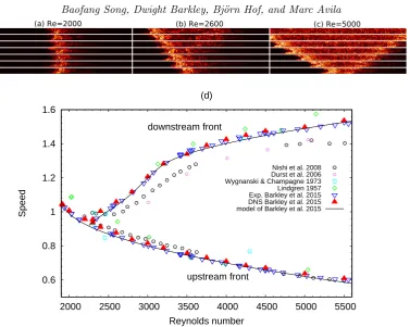
Figure 1.Temporal evolution of (a) a puff atRe= 2000, (b) a slug atRe= 2600, and (c) a
slug atRe= 5000. The flow is from left to right, and turbulence is visualised by the transverse turbulent fluctuationsq (defined in§2.1) in a frame of reference co-moving at the average of the upstream and downstream front speeds. The length scale in the vertical (radial) direction is stretched by a factor of 2 for better visualisation. Dark areas correspond to small fluctuations and bright areas correspond to large fluctuations. Time evolves in the upward direction and panels are separated by 10D/U in (a, c) and by 100D/U in (b), whereU is the bulk velocity and D the pipe diameter. (d) Front speeds as a function of Reynolds number taken from the literature as indicated.
persistent turbulent state (see figure 1c). In their seminal experimental work Wygnanski & Champagne (1973) investigated the energy budget of slugs. Their measurements above Reynolds number 4200 (atRe= 4.2×10³,Re= 2×10⁴, andRe= 2.32×10⁴based on
the bulk velocity U and pipe diameter D) showed that the upstream and downstream
fronts of slugs have a similar, well-defined structure. They observed that within the bulk region there is sufficient turbulent kinetic energy production to sustain turbulence and hence that the bulk region corresponds to that of fully turbulent pipe flow.
Duguet et al. (2010) conducted detailed direct numerical simulations of slug forma-tion and noted that slugs take multiple forms as manifested by different downstream front structures. At moderate Reynolds numbers slugs have diffusive downstream fronts, not unlike the downstream fronts observed for puffs (see figure 1b), whereas at high Reynolds numbers the downstream fronts are sharper, with a well-defined structure sim-ilar in intensity to the upstream fronts (see figure 1c). This variation in the structure of downstream fronts can be clearly seen in earlier experimental work (e.g. Nishi et al.
as weak fronts and the sharper form as strong fronts. The corresponding slugs are thereby called weak and strong slugs, respectively.
The origin of the various structures has recently been elucidated with the guide of an advection-reaction-diffusion model (Barkley 2011; Barkley et al. 2015). Figure 1(c) illustrates this sequence by showing the speeds of upstream and downstream fronts as a function of Reynolds number. Points show measurements from a variety of past studies. The up and down triangles are from recent experiments and direct numerical simulations aimed at accurately resolving the details of front speeds within the transitional regime. The corresponding model analysis is shown with solid curves. At low Reynolds numbers (Re . 2250) turbulence is localised in the form of puffs and hence the upstream and downstream front speeds are identical. Both front speeds decrease with increasingRe.
As Re is increased above Re ' 2250, the downstream front speed begins to abruptly
increase withRe, thereby deviating from the upstream front speed. This marks the onset of expanding turbulent slugs. Within the model analysis, this transition from puffs to slugs is understood as a change from excitability to bistability. Initially, for Re only slightly aboveRe '2250 turbulent slugs take the weak form and the expansion rate of the turbulent structure is modest. (See figure 1(b) and note that the time scale here is 10 times larger than that of the other two visualisations.) At high Reynolds numbers expansion is much more rapid and the slugs take the strong form with sharp fronts at both upstream and downstream ends (figure 1c). For a comprehensive discussion on the model and theoretical perspective of the route to turbulence in pipe flow, see Barkley (2016).
The focus of the current work is the distinction between weak and strong slugs. Al-though the dynamics of weak and strong fronts was described within a model system, further study of real pipe flow is essential to elucidate the physical mechanisms distin-guishing them. The issues are the following. Firstly, the model is only one dimensional, whereas in reality fronts are evolving in a highly complicated fashion and are spatially convoluted (Holzner et al. 2013). This complexity results from three dimensionality of the interface and intrinsic turbulent fluctuations and that cannot be fully captured by the one-dimensional model. Hence it is important to compare model fronts with those from full simulations of the Navier–Stokes equations. Secondly, and more importantly, the model assumes certain physical properties of turbulent pipe flow that we establish as facts for the first time in the present work. Specifically, here we carry out extensive direct numerical simulations (DNS) of the Navier–Stokes equations to analyse the physics of the laminar-turbulent fronts of slugs. Through the analysis we elucidate the key distinction between weak and strong fronts, both in terms of the kinetic energy budget across the fronts and in terms of front motion relative to the advection speed turbulent structures within the bulk.
2. Characterisation of front types
2.1. Preliminaries
In principle the simulations could be initiated in multiple ways, for example, by a forc-ing that mimics wall injection in the laboratory experiments (e.g. Darbyshire & Mullin (1995); Hof et al. (2003); Hanet al. (2000); Reuter & Rempfer (2004); Mellibovsky & Meseguer (2007)), or by perturbing laminar flow with localised pair of streamwise rolls (e.g. Mellibovskyet al.(2009)). In our case, the initial conditions are all taken to be snap-shots from turbulent puff simulations at a fixed Reynolds number (Re = 2000), so that initial conditions resemble the snapshots shown in figure 1(a). In this way all initial con-ditions are already fully nonlinear turbulent states of nearly identical streamwise extent and amplitude. Such initial conditions always transform rapidly into slugs in simulations at higher Reynolds number. The initial transients corresponding to the transformation into slugs are excluded from the analysis. Then 150 to 500 snapshots of each expand-ing slug are recorded. (We used a 180D-long pipe with periodic boundary conditions in the streamwise direction for all simulations. The number of snapshots depends on how quickly the slug length grows and fills the whole domain. Hence the number decreases with increasingRe.) For further details, see Barkley et al. (2015). For the phase-plane plots that appear in §2.2, we re-analyse the same data set generated by Barkley et al.
(2015) who used the data to obtain the front speeds shown in figure 1(d). For the the energy budget analysis in §3 and for the advection speeds computations in§4, further computations have been performed using the same computational techniques.
From the DNS data, we use
q(z) :=
s Z Z
(u2
r+u2θ)rdrdθ
as an indicator of the local turbulence intensity along the pipe axis, where r, θ, z are radial, azimuthal, and axial coordinates, and ur and uθ are the radial and azimuthal velocity components, (non-dimensionalised by the bulk velocityU).
As proposed by Barkley (2011) the turbulence intensity, q, and the axial centreline velocity,u=uz(r= 0), provide a convenient and compact characterisation of the state of the flow. For fully developed laminar flowq= 0 andu= 2, while for a turbulent flow,
q > 0 and u < 2. The lower value of uin the turbulent case results from a plug-like
velocity profile corresponding to a lower mean shear in the turbulent state.
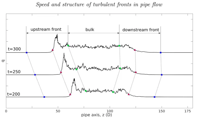
Because turbulent slugs are not fixed structures but expand over time, for our analysis it is necessary to divide a turbulent slug into three parts: upstream front, bulk, and downstream front (see figure 2). A position for the laminar-turbulent fronts can be defined by setting a threshold inqabove which the flow is considered as turbulent. We have used the threshold valueq= 2×10⁻², but we have verified that none the results that are to
follow are sensitive to the precise value of the threshold, for a substantial range of values. The upstream and downstream front regions are then taken to be of fixed streamwise extent (40D), while the size of the bulk region varies with time. The relationship between q andu is numerically obtained separately in each of the three regions. To remove the effect of fluctuations and determine the mean dynamics of the fronts, we compute average over time (the saved snapshots) and the ensemble of runs.
2.2. Fronts in the u-qphase plane
Figure 2.Division of a slug into upstream front, bulk and downstream front. A slug atRe=2800
is plotted at three time instants in a reference frame co-moving with the bulk flow. The flow is from left to right. Red triangles mark the position of the upstream and downstream fronts given by the cutoffq= 0.02. The bulk region is bounded between green circles, which are located 15D to the inside relative to the front positions (red triangles). Blue squares mark the beginning of the fronts and are located 25Dto the outside relative to the front positions. With these choices the fronts span 40Din length.
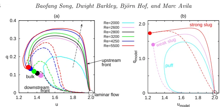
Referring to figure 3(a), starting from the parabolic laminar flow on the upstream side, there is a sharp increase in turbulence intensityq across the upstream front while the centreline velocityuremains almost unchanged. This is as expected since the modification of the mean shear must respond to the turbulent fluctuations. This rise inqoccurs both for slugs and for puffs. For puffs the rise is rather moderate (see the cyan curve for
Re = 2000 in figure 3a), while for slugs, the rise is both larger and steeper. For slugs, the value of u decreases by less than 5% during the rise of q, in agreement with the measurements of Wygnanski & Champagne (1973). Following this sharp jump inq, the centreline velocityudecreases, corresponding to a blunting of the shear profile in response to the high level of turbulence excitations. Subsequently, both uand q gradually level off in the bulk part of the structure shown with points in the phase plot. The constant levels of qanduin the bulk indicate that turbulence production and dissipation are in balance. In fact, the values ofuandqindicated by points are identical to those obtained from simulations of fully turbulent pipe flow at the corresponding Reynolds number.
0 0.1 0.2 0.3 0.4
1.2 1.4 1.6 1.8 2.0
q
u (a)
upstream front
downstream front
laminar flow bulk
Re=2000 Re=2600 Re=2800 Re=3200 Re=4250 Re=5500
0 1.0 2.0
1.2 1.4 1.6 1.8 2.0
qmodel
umodel
(b)
strong slug
weak slug
[image:7.595.100.465.101.278.2]puff
Figure 3.(a) The structure of turbulent-laminar fronts from DNS seen as trajectories in the
(u, q)-phase plane. Upstream fronts for slugs are shown with solid lines while downstream fronts are shown as dashed lines. Filled circles correspond to the bulk region of the slug. The dashed arrow indicates the direction of increasing Reynolds number. The turbulent puff atRe= 2000 does not have a bulk region and for this case we do not distinguish upstream and downstream fronts with different line types. Trajectories form counterclockwise loops in the phase plane as one travels in space from the upstream to the downstream along the pipe. Phase-space trajectories have been obtained by averaging over time and over multiple runs at eachRe(typically 20 runs with 150 to 500 snapshots per run, depending on Re). (b) For comparison, the structure of turbulent-laminar fronts from a model of turbulent pipe flow (Barkley 2016). The trajectories are taken directly from Barkley (2016) figure 20.
AsRe increases, the overshoot ofqacross the downstream front becomes increasingly sharp and the shape of the curveq(u) becomes very close to that of the upstream front. (The upstream front is always of strong type.) This is in agreement with Wygnanski & Champagne (1973), who measured the streamwise velocity profile of upstream and downstream fronts forRe >4200 in anr-zpipe cross-section and showed that they were similar.
For comparison, in figure 3(b) we show phase plane trajectories for a model puff, weak slug, and strong slug typical of those from the model of pipe flow proposed in Barkley
et al. (2015) and discussed in detail in Barkley (2016). While the model captures the qualitative essence of the three states (a closed loop for a puff, a monotonic decay of q for a weak downstream front and increase ofq before dropping for a strong downstream front), it is clear that the model fails to capture quantitatively the structure of fronts from full DNS. The fact that the model value ofq do not agree with those from DNS is not significant, as this could be accounted for with some straightforward rescaling. What is significant is that the strong overshoots in q observed in the DNS are missed by the model. This shows that further work is needed to obtain a model that quantitatively captures the fronts in turbulent pipe flow.
2.3. Dynamic switching between weak and strong fronts
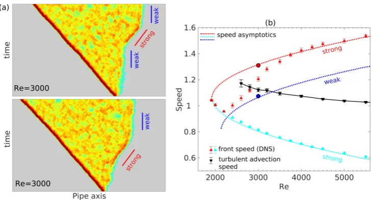
Figure 4. Switching between weak and strong front atRe = 3000. (a) Space-time diagrams showing the colourmap ofq for two typical slugs in a moving frame of reference with the speed of 1.06U (the speed of the weak front at this Reynolds number). Grey areas correspond to small fluctuations and dark red areas correspond to large fluctuations. The bars show the slopes, i.e. the inverse of the speeds, of transient weak and strong fronts in this frame of reference. (b) Front speed as a function of Reynolds number from DNS (up-triangles) and from an asymptotic analysis of fronts in a model system (dotted lines), reproduced from Barkley et al. (2015). The circles show the speeds of the transient weak and strong fronts highlighted in (a). Black down-triangles show the mean turbulent advection speed in the bulk region of slugs computed using equation (4.2) and discussed in§4
behaviour has not been reported previously and was not observed in modelling studies. The speeds of these two front types have been determined separately and are plotted on the speed diagram of figure 4(b) as separate circles. They lie almost perfectly on the weak and strong speed asymptotics predicted by the theory of Barkley et al. (2015), who considered the limit of infinitesimally thin fronts. In this limitqis a discontinuous function ofuinstead of a steep but continuous function as shown in figure 3(a). As the front transiently takes one of the two forms, the ensemble average speed (the red up-triangle atRe = 3000 in figure4(b)) sits between the two asymptotic values. Our DNS data show that for 2800<Re <3200 dynamic switches in downstream front type are often observed. Outside of this range we find almost entirely constant downstream front types, weak fronts at low Re and strong fronts at high Re. The marked differences in propagation speed and turbulent intensity between the two front types calls for a deeper investigation of the physical distinction between them, which we address in the following sections.
3. Energy budget at the fronts
access to temporally and spatially resolved data, which motivates us to revisit their turbulent kinetic energy budget in order to shed light on the origin of the different turbulent intensity profiles at weak and strong fronts.
Here we use the Reynolds decomposition of the velocity fieldu= ¯u+u0whereuis the total velocity, ¯uis the mean velocity field averaged over time and over the homogeneous (azimuthal) direction, andu0 is the fluctuation with respect to the mean. The equation of the mean turbulent kinetic energyk= 12u0·u0 reads (Pope 2000, pp.123-128):
¯ Dk
¯
Dt +∇ ·T =P−, (3.1)
where D¯D¯t= ∂t∂ + ¯u· ∇is the material derivative associated with ¯u, and
Ti =
1 2u
0
iu0ju0j+u0ip0− 2
Reu
0
jsij (3.2)
is the mean energy flux due to diffusion and the work by fluctuating pressurep0 through the surface of a fixed control volume. Here the Einstein summation convention is used and
sij =
1 2 ∂u0 i ∂xj +∂u 0 j ∂xi (3.3)
is the fluctuating rate of strain. The production term and dissipation term are
P=−u0iu0j∂ui ∂xj
, = 2
Resijsij. (3.4)
We note that Wygnanski & Champagne (1973) defined the dissipation as
˜ = 1 Re ∂u0 i ∂xj ∂u0 i ∂xj −1 2
∂2(u0
iu0i) ∂xj∂xj
(3.5)
which does not fully account for the viscous dissipation in turbulence and mixes vis-cous dissipation and energy flux (transport) due to diffusion. As a result their analysis underestimated dissipation.
In the frame of reference co-moving with the fronts at velocity UF, the equation for
the mean kinetic energy of the turbulent fluctuations reads
∂k
∂t =P−−( ¯u−UF)· ∇k− ∇ ·T = 0, (3.6) as the fronts are in statistical equilibrium in this frame of reference.
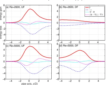
Figure 5 shows the cross-sectionally integrated energy budget for turbulent fronts at
Re = 2600 (a, b) andRe = 5000 (c, d). In the figure, laminar flow is on the left for the upstream front (a, c), and on the right for the downstream front (b, d). In the formulation of Pope (2000) used here, production and dissipation are the source and sink terms in the energy budget and our calculation shows that they are comparable in magnitude at all axial positions. This is in contrast to the calculation of Wygnanski & Champagne (1973), who reported that dissipation is orders of magnitude smaller than production at the fronts (see Table 1 and 2 in their paper). We believe that this discrepancy is due to their definition of the dissipation term.
−4 −2 0 2 4 −6
−4 −2 0 2 4 6
(b) Re=2600, DF P
−ǫ
-∇·T
-(u−UF)·∇k
−4 −2 0 2 4
−6 −4 −2 0 2 4 6
energy loss energy gain
(a) Re=2600, UF
−4 −2 0 2 4
−6 −4 −2 0 2 4 6
(d) Re=5000, DF
−4 −2 0 2 4
−6 −4 −2 0 2 4 6
[image:10.595.108.472.114.396.2]pipe axis, z(D) (c) Re=5000, UF
Figure 5.Kinetic energy budget (integrated over pipe cross-section) in the frame of reference
co-moving with the fronts. Production (red bold line), dissipation (blue dash-dotted line), energy flux (cyan thin line), and convection (violet dashed line) are normalised by the mean turbulence production rate in the bulk. (a, b) Upstream front (UF) and downstream front (DF) of a slug atRe= 2600. (c, d) Upstream front and downstream front of a slug atRe= 5000. In (a, c, d) the peak of the production term is positioned atz= 0. At each Reynolds number, an ensemble of about 500 snapshots is used to perform the energy budget analysis.
are large eddies at the strong fronts extracting energy from the adjacent laminar flow (see figure 6 and online supplementary movies). As one moves further towards the bulk, the energy production rate decreases and dissipation outweighs production. As a result the turbulence intensity decreases and the strong front eventually manifests an intensity peak (see figure 3 and figure 4). Production and dissipation eventually level off in the bulk and come into balance, while the energy flux and convection vanish as the equilibrium (fully developed) profile is reached. All terms in the energy budget for upstream and strong downstream fronts exhibit essentially the same streamwise variation, (apart from the obvious streamwise reflection symmetry). This in turn is responsible for their very similar shape in theu-qphase plane shown in figure 3.
Figure 6.Advection of vortices near weak and strong fronts. (a) Weak front atRe= 2600, (b)
strong front atRe= 5000. Vortices, visualised by using the Λ2criterion, are shown in the frame
of reference co-moving with the downstream front (time evolves in the upward direction). The bulk turbulent region is on the left and the downstream laminar flow is on the right. In each case one vortex is highlighted by red colour and a circle and is tracked in time. In (a) the time separation between two consecutive panels is 1.5D/U, whereas in (b) it is 0.625D/U.
4. Fronts in the frame moving at the bulk turbulent advection speed
The energy budget analysis shows that weak and strong fronts can be clearly distin-guished by the streamwise variation in the turbulence production and dissipation. To shed light on the origin of this difference, we here investigate the dynamics of turbulent vortices near downstream fronts. Figure 6(a)–(b) show isosurfaces of Λ2 at four timeinstants in a frame co-moving with the downstream front at Re = 2600 and 5000, re-spectively. In each case, one of the vortices has been coloured red and circled so as to highlight its motion relative to the front. In theRe= 2600 case, the vortex is generated within the turbulent core. Because it travels faster downstream than the downstream front, it moves towards the front. Eventually it will abandon the turbulent slug at the front. Similar relative motion of the vortices with respective to the fronts for puffs was also observed in Hofet al.(2010). By contrast, atRe= 5000 the vortex is generated at the downstream front and travels away from the front and into the turbulent bulk. The dynamics of these two specific vortices is representative of advecting structures at their respective Reynolds numbers (see supplementary online movie), and suggests that, in addition to the energy budget, weak and strong front can be distinguished by the speed at which vortices are advected relative to the downstream front speed.
In wall-bounded shear flows the advection speed of turbulent structures (vortices and streaks) depends on their size and distance from the wall (Del ´Alamo & Jim´enez 2009; Peiet al. 2012). However, Del ´Alamo & Jim´enez (2009) showed that only small vortices exhibit a clear radial dependence in their advection speed, whereas relatively large vor-tices are in fact advected at a rather uniform speed (also evidenced in Duguet et al.
(2010)). Recently, Del ´Alamo & Jim´enez (2009); Kreiloset al.(2014) proposed a method to define and remove the mean advection speed of turbulence in parallel shear flows.
Starting from the Navier–Stokes equation
∂tu(r, θ, z, t) =−u· ∇u− ∇p+
1
Re∇
2u (4.1)
1.0 1.1 1.2 1.3 1.4 1.5 1.6
3000 4000 5000
speed (U)
Reynolds number (a)
advection velocity c ucentreline
-0.6 -0.4 -0.2 0 0.2
3000 4000 5000
c-u
centreline
(U)
[image:12.595.107.462.127.281.2]Reynolds number (b)
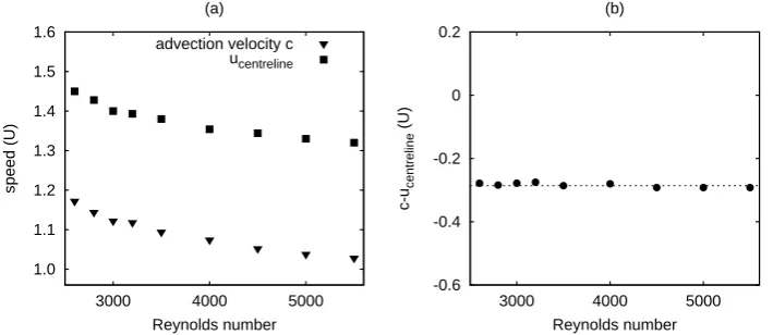
Figure 7.Comparison between the average turbulent advection speed and the average centreline
velocity as a function of Re. (b) Difference between the advection speed and the centreline velocity.
speed can be computed as
c=−< ∂zu(r, θ, z, t)·f(u(r, θ, z, t), p, t)> k∂zu(r, θ, z, t)k2
. (4.2)
Here the inner product and 2-norm of vector fields a and b are defined as <a·b>=
R
V(a·b)dV and kak
2 =<a·a >. Note that equation (4.2) is obtained by minimising
u(r, θ, z+ ∆z, t+ ∆t)−u(r, θ, z, t) in the discrete form
< ∂zu(r, θ, z, t)·(u(r, θ, z+ ∆z, t+ ∆t)−u(r, θ, z, t))>= 0,
with ∆z=c∆t.
This method allows the calculation of an instantaneous mean turbulent advection speed using only a single velocity snapshot and the local time derivatives, therefore, has advantages compared to the methods based on calculating the velocity correlation between flow fields with a proper time separation, which is not known a priori and introduces uncertainties (see e.g., Kim & Hussain (1993); Peiet al.(2012). It has been shown to be able to precisely obtain the advection speed of a travelling wave solution in channel flow (Kreiloset al.2014).
The black down-triangles in figure 4(b) and figure 7(a) show the mean turbulent ad-vection speed as a function of the Reynolds number obtained with equation 4.2. The computations are for fully turbulent pipe flow and give the speed of the bulk turbulent structures. These calculations reveal a simple relation between the average turbulent advection speed and the average centreline velocity in the bulk (see figure 7(b)),
c=ucentreline−(0.286±0.008), (4.3)
where 0.008 is the standard deviation of the speed difference. This relation holds in the whole range of Reynolds numbers investigated. It should be noted that for the purposes of modelling, Barkleyet al.(2015) and Barkley (2016) assumed that turbulence is advected more slowly than the centreline velocity by a fixed constant. The results here demonstrate that this is in fact the case.
move. As seen in figure 4(b), at lowRe.2900, mean turbulent advection speedcis larger than the speeds of both upstream front (cyan up-triangles) and downstream front (red up-triangles). Hence, in the frame in which the bulk turbulent structures are stationary, both fronts move to the left (upstream direction). New turbulent structures are generated at the upstream front as it moves to the left. These structures then decay back to laminar flow as the downstream front subsequently passes. ForRe&2900 the speed of the strong front is larger than c. Hence, in the frame in which the bulk turbulent structures are stationary, downstream fronts now moves to the right (downstream direction), generating new turbulent structures. Hence turbulent structures are now generated at both fronts and the large eddies produced at the fronts extract energy from the adjacent laminar flow, on both the upstream and downstream end of the slug, in agreement with the energy budget analysis. This strong correlation between front speed and turbulence intensity can also be seen in the colourmap of figure 4: the strong front is red (highq), whereas the weak front is yellow. From our argument it could thus be inferred that weak slugs feature a decaying downstream front whereas strong slugs possess a turbulence-producing downstream front, and the transition between weak and strong fronts should occur at
Re ≈ 2900. Our data support this argument and indeed below 2900, weak fronts are
(statistically) more likely to occur, while strong fronts dominate above 2900.
5. Discussion and conclusion
By performing and analysing extensive direct numerical simulations, we have studied the propagation and structure of laminar-turbulent fronts in pipe flow over a wide range
of Reynolds numbers, from Re = 2000 to Re = 5500. The structure of the upstream
front remains qualitatively unchanged over the whole Reynolds number range and its dimensionless speed monotonically decreases as Re increases. The main feature of this front is a sharp peak in turbulent intensity, which is due to the ability of the upstream front to extract energy from the upstream laminar flow. As a result turbulent production is at the upstream front much larger than in the bulk. Dissipation within the upstream front is similar in magnitude to production, but the peak dissipation is reached down-stream of the peak production. This effect has been missed in prior studies. This delay arises because the energy is transferred from the large eddies at the interface down to the smallest scales as the turbulent structures are advected downstream.
The behaviour of the downstream front is more complex and changes drastically as the Reynolds number increases. At low Reynolds numbers the downstream front of slugs is weak, i.e. consisting of a gradual relaminarisation toward the parabolic flow profile as seen in puffs. Interestingly, we have found that turbulence is locally in equilibrium at weak fronts: at each streamwise location production and dissipation balance and there is no streamwise transport of kinetic energy by diffusion or convection. AsReincreases, strong downstream fronts, characterised by a peak in turbulent intensity similar to that of upstream fronts, are found to dominate.
that a different definition of dissipation was used by Wygnanski, which does not fully account for the viscous dissipation in turbulence. As a result (Wygnanski & Champagne 1973) underestimated dissipation at the fronts, which led them to conclude that there is a large net production at strong fronts.
Based on a comparison between the advection speed of turbulence in the bulk of slugs and the speed of fronts, our study reveals the fundamental mechanism of transition be-tween weak and strong fronts. ForRe.2900 the downstream front travels slower than the bulk turbulent advection speed and so in the co-moving frame, turbulence relaminarises along the weak front. In contrast, forRe&2900 the downstream front travels faster than the bulk turbulent advection speed and so it can aggressively invade the laminar flow ahead, while extracting energy from it just as the upstream front does. In the interme-diate regime aroundRe '2900, fluctuations of turbulence production/dissipation, may cause temporal switching between the two types of front (see figure 4). Hence the tran-sition from weak to strong fronts is of statistical nature, exactly as the trantran-sition from transient to sustained turbulence (Avila et al. 2011) or the onset of weakly expanding slugs (Barkleyet al.2015).
Our study has been restricted to pipe flow, but we believe that the front dynamics and physical mechanisms shown here are generic to wall-bounded turbulent flows. Ex-periments in square ducts display both types of fronts and hence support this hypothesis (Barkley et al. 2015). In flows with two spatially extended dimensions, such as chan-nel and Couette flows, advection is possible in the spanwise and streamwise directions (Barkley & Tuckerman 2007; Duguet & Schlatter 2013), resulting in substantially more complex front dynamics and challenging current modelling strategies.
Acknowledgements
We thank Dr. Ashley P. Willis for sharing his spectral toroidal-poloidal pipe flow code and Anna Guseva for reading the manuscript. We acknowledge the Deutsche Forschungs-gemeinschaft (Project No. FOR 1182), and the European Research Council under the European Unions Seventh Framework Programme (FP/2007-2013)/ERC Grant Agree-ment 306589 for financial support. B. S. acknowledges financial support from the Chinese State Scholarship Fund under grant number 2010629145, support from the Max Planck Society and the Institute of Science and Technology Austria (IST Austria). We acknowl-edge the computing resources from Gesellschaft f¨ur wissenschaftliche Datenverarbeitung G¨ottingen (GWDG), the J¨ulich Supercomputing Centre (grant HGU16), the Regionalen Rechenzentrums Erlangen (RRZE) and computing facilities at IST Austria.
REFERENCES
Avila, K., Moxey, D., De Lozar, A., Avila, M., Barkley, D. & Hof, B.2011 The onset of turbulence in pipe flow.Science 333, 192–196.
Barkley, D.2011 Simplifying the complexity of pipe flow.Phys. Rev. E 84, 016309.
Barkley, D.2016 Theoretical perspective on the route to turbulence in a pipe.J. Fluid Mech.
803, P1.
Barkley, D., Song, B., Mukund, V., Lemoult, G., Avila, M. & Hof, B.2015 The rise of fully turbulent flow.Nature526, 550–553.
Barkley, D. & Tuckerman, L. S. 2007 Mean flow of turbulent-laminar patterns in plane
Couette flow.J. Fluid Mech.576, 109–137.
Darbyshire, A. G. & Mullin, T. 1995 Transition to turbulence in constant-mass-flux pipe
Del ´Alamo, J. C. & Jim´enez, J. 2009 Estimation of turbulent convection velocities and
corrections to Taylor’s approximation.J. Fluid Mech.640, 5–26.
van Doorne, C. W. H. & Westerweel, J.2009 The flow structure of a puff.Phil. Trans. R. Soc. A367, 489–507.
Duguet, Y. & Schlatter, P.2013 Oblique laminar-turbulent interfaces in plane shear flows.
Phys. Rev. Lett.110, 034502.
Duguet, Y., Willis, A. P. & Kerswell, R. R.2010 Slug genesis in cylindrical pipe flow.
J. Fluid Mech.663, 180–208.
Durst, F. & ¨Unsal, B. 2006 Forced laminar to turbulent transition in pipe flows. J. Fluid
Mech.560, 449–464.
Han, G., Tumin, A. & Wygnanski, I.2000 Laminar-turbulent transition in Poiseuille pipe flow subjected to periodic perturbation emanating from the wall. Part 2. Late stage of transition.J. Fluid Mech.419, 1–27.
Hof, B., De Lozar, A., Avila, M., T, X. & Schneider, T. M.2010 Eliminating turbulence
in spatially intermittent flows.Science 327, 1491–1494.
Hof, B., Juel, A. & Mullin, T.2003 Scaling of the turbulence transition threshold in a pipe.
Phys. Rev. Lett.91, 244502.
Holzner, M., Song, B., Avila, M. & Hof, B.2013 Lagrangian approach to laminar-turbulent interfaces.J. Fluid Mech.723, 140–162.
Kim, J. & Hussain, F.1993 Propagation velocity of perturbations in turbulent channel flow.
Phys. Fluids5, 695–706.
Kreilos, T., Zammert, S. & Eckhardt, B. 2014 Comoving frames and symmetry-related motions in parallel shear flows.J. Fluid Mech.751, 685–697.
Lindgren, E. R.1969 Propagation velocity of turbulent slugs and streaks in transition pipe flow.Phys. Fluids 12, 418.
Mellibovsky, F. & Meseguer, A. 2007 Pipe flow transition threshold following localized
impulsive perturbations.Phys. Fluids19, 044102.
Mellibovsky, F., Meseguer, A., Schneider, T. M. & Eckhardt, B. 2009 Transition in localized pipe flow turbulence.Phys. Rev. Lett.103, 054502.
Nishi, M., ¨Unsal, B., Durst, F. & Biswas, G.2008 Laminar-to-turbulent transition of pipe flows through puffs and slugs.J. Fluid Mech.614, 425–446.
Pei, J., Chen, J., She, Z.-S. & Hussain, F.2012 Model for propagation speed in turbulent
channel flows.Phys. Rev. E 86, 046307.
Pope, S. B.2000Turbulent flows. Cambridge university press.
Reuter, J. & Rempfer, D. 2004 Analysis of pipe flow transition. Part I. Direct numerical simulation.Theoretical and Computational Fluid Dynamics 17, 273–292.
Rotta, J.1956 Experimenteller beitrag zur entstehung turbulenter str¨omung im rohr.Ing.-Arch
24, 258–82.
Sreenivasan, K. R. & Ramshankar, R. 1986 Transition intermittency in open flows, and intermittency routes to chaos.Physica 23D, 246–258.
Willis, A. P. 20xx The openpipeflow.org Navier-Stokes solver. Tech. Rep.. Open-pipeflow.org/index.php?title=File:TheOpenpipeflowSolver.pdf.
Willis, A. P. & Kerswell, R. R.2009 Turbulent dynamics of pipe flow captured in a reduced
model: puff relaminarisation and localised ‘edge’ states.J. Fluid Mech.619, 213–233.
Wygnanski, I. J. & Champagne, F. H.1973 On transition in a pipe. Part 1. The origin of puffs and slugs and the flow in a turbulent slug.J. Fluid Mech.59, 281–335.
Wygnanski, I. J., Sokolov, M. & Friedman, D.1975 On transition in a pipe. Part 2. The