Some spatial statistical techniques with applications to cellular imaging data

(1)

warwick.ac.uk/lib-publications

A Thesis Submitted for the Degree of PhD at the University of Warwick

Permanent WRAP URL:

http://wrap.warwick.ac.uk/97940

Copyright and reuse:

This thesis is made available online and is protected by original copyright.

Please scroll down to view the document itself.

Please refer to the repository record for this item for information to help you to cite it.

Our policy information is available from the repository home page.

(2)

Some spatial statistical

techniques with applications to

cellular imaging data

Thomas Honnor

A thesis presented in fulfilment of the requirements for

the degree of

Doctor of Philosophy in Statistics

Department of Statistics

University of Warwick

(3)

List of Figures

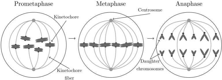
1.1 Diagram of the intermediate stages of mitosis . . . 2

3.1 Diagrams of simulated point pattern realisations . . . 49

3.2 Diagram of some observed point patterns . . . 55

3.3 Diagram of an observed marked point pattern . . . 56

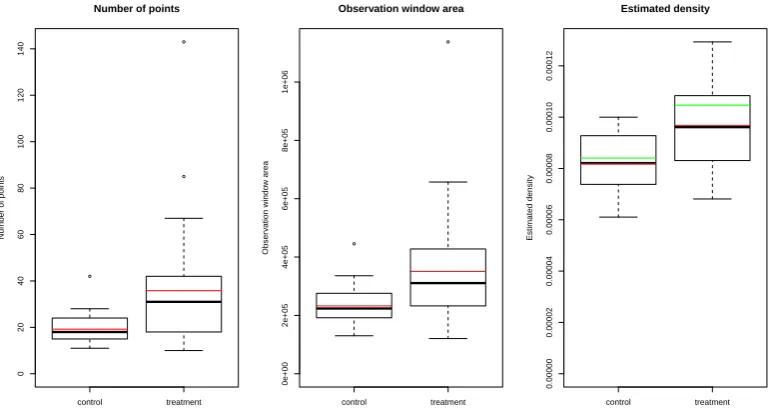
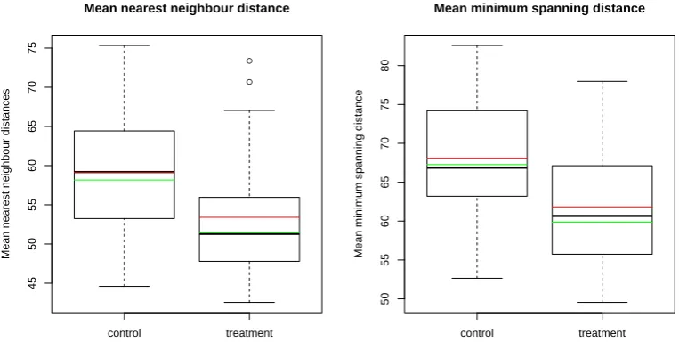
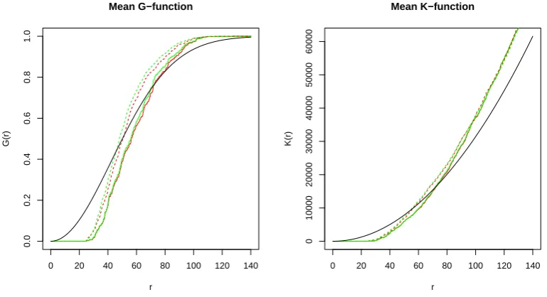
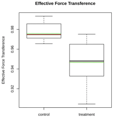
3.4 Plots of first order point pattern summary statistics for observed data 60 3.5 Plots of point separation distance summary statistics for observed data 61 3.6 Plots of second order summary functions for observed data . . . 62

3.7 Plot of marked point pattern summary statistics for observed data . 63 4.1 Diagram illustrating the temporal evolution of a simulated spatio-temporal process and the resulting summary statistic . . . 76

4.2 Diagram illustrating transformations permittable under the symme-tric null hypothesis and the resulting equivalence classes of subregions 82 4.3 Images of spatio-temporal process simulations . . . 88

4.4 Diagrams of true and estimated movement patterns for a simulated spatio-temporal process . . . 89

4.5 Images of observed spatio-temporal processes across five consecutive time points for three samples . . . 98

4.6 Plot of colocalisation between observed data as measured by Pearson’s correlation coefficient . . . 100

4.7 Plots of temporal variation in subregion intensity for observed data . 101 5.1 Diagram of proposed transformation of observed line pattern data to a standardised coordiante system . . . 110

5.2 Diagram of discrepancy between mitotic spindle model and observed data directions . . . 112

5.3 Diagram of observed data for a sample with good model fit . . . 114

(7)

5.5 Plot of smoothed, normalised density estimates of angles between

(8)

List of Tables

3.1 Summary of validation study results for point patterns . . . 52

3.2 Summary of validation study results for marked point patterns . . . 53

3.3 Test results for observed (marked) point pattern data . . . 63

3.4 Treatment effect sizes for observed (marked) point pattern data . . . 65

3.5 Summary of sensitivity analysis results for (marked) point pattern data 68

4.1 Summary of test results for independent spatio-temporal simulations

under a variety of null hypotheses . . . 92

4.2 Summary of test results for dependent spatio-temporal simulations

under the most appropriate null hypothesis . . . 94

4.3 Summary of test results for dependent isotropic spatio-temporal

si-mulations tested under a number of suitable null hypotheses . . . 96

4.4 Summary of test results for observed data . . . 103

5.1 Mitotic spindle model fit comparison scores between observed data

(9)

Acknowledgements

I would like to thank my supervisors, Dr. Julia Brettschneider and Dr. Adam

Johansen; collaborators, Dr. Stephen Royle and his research group; department

colleagues; friends and family for all of their help and support over the course of my

studies. This thesis would not have been possible without you.

Particular thanks go to Dr. Stephen Royle and his research group within the

Centre for Mechanochemical Cell Biology at the University of Warwick for

discussi-ons of the biological and statistical problems of interest to them and for providing

the data that serves to illustrate the ability of the methodologies proposed within

this thesis.

I would also like to thank the Engineering and Physical Sciences Research

Coun-cil for funding these studies through Doctoral Training Grants EP/K503204/1,

(10)

Declarations

This thesis is submitted to the University of Warwick in support of my application

for the degree of Doctor of Philosophy. It has been composed by myself and has not

been submitted in any previous application for any degree.

The work presented was carried out by the author, with real biological data

made available by Dr. Stephen Royle, Department of Mechanochemical Cell Biology,

University of Warwick.

Material from Chapters 3 and 4 respectively has been made available by the

author as working papers:

Thomas R. Honnor, Julia A. Brettschneider, Adam M. Johansen,

Differen-ces in spatial point patterns with application to subcellular biological structures,CRiSM Working Paper 17-01.

Thomas R. Honnor, Adam M. Johansen, Julia A. Brettschneider, A

non-parametric test for dependency between estimated local bulk movement patterns,CRiSM Working Paper 17-03.

Material from Chapter 5 has been published by the author in the following paper:

F. M. Nixon, T. R. Honnor, N. I. Clarke, G. P. Starling, A. J. Beckett, A. M. Johansen, J. A. Brettschneider, I. A. Prior, and S. J. Royle. Microtubule

or-ganization within mitotic spindles revealed by serial block face scanning electron

microscopy and image analysis. Journal of Cell Science, 130(10):1845-1855, April

(11)

Abstract

The aim of this thesis is to provide techniques for the analysis of a variety of types of

spatial data, each corresponding to one of three biological questions on the function

of the protein TACC3 during mitosis. A starting point in each investigation is

the interpretation of the biological question and understanding of the form of the

available data, from which a mathematical representation of data and corresponding

statistical problem are developed.

The thesis begins with description of a methodology for application to two

col-lections of (marked) point patterns to determine the significance of differences in

their structure, achieved through comparison of summary statistics and

quantifica-tion of the significance of such differences by permutaquantifica-tion tests. A methodology is

then proposed for application to a pair spatio-temporal processes to estimate their

individual temporal evolutions, including ideas from optimal transportation theory,

and a test of dependence between such estimators. The thesis concludes with a

proposed model for line data, designed to approximate the mitotic spindle structure

using trajectories on the surface of spheroids, and a comparison score to compare

model fit between models and/or observations.

The results of methodologies when applied to simulated data are presented as

part of investigations into their validity and power. Application to biological data

indicates that TACC3 influences microtubule structure during mitosis at a range of

scales, supporting and extending previous investigations.

Each of the methodologies is designed to require minimal assumptions and

num-bers of parameters, resulting in techniques which may be applied more widely to

(12)

Chapter 1

Introduction

State of the art microscope technology allows the collection of large numbers of

high resolution images. Specialised preparation of biological samples and choice of

imaging approach can lead to the identification of subcellular structures and the

localisation of biomolecular species within such images. The purpose of collecting

such images may be observational, to ascertain the typical behaviour within the cell,

or experimental, to ascertain the impact on the cell of applied external conditions.

It is commonly the case that images are collected from multiple samples, the

ana-lysis of which may be improved in terms of accuracy and reliability by statistical

techniques. This thesis combines three investigations of spatial data arising from

images of biological samples during mitosis and formulates statistical methodologies

for their analysis to answer related biological questions of interest.

1.1 Biological background

Mitosis is the procedure through which eukaryote cells (those within fungi, plants

and animals) replicate, with one cell dividing into two. Chromosomes encode the

genetic material within cells and during mitosis the collection of chromosome pairs

are divided such that one chromosome from each pair makes its way into each of the

two resulting cells. Errors in the division of chromosome pairs can result in the death

of resulting cells or mutations that may be harmful to the organism (Holland and

Cleveland, 2009). A key research topic for cell biologists is therefore the process of

mitosis, the action of biomolecular species during mitosis and the impact of applied

external conditions on the process.

Division of chromosome pairs during mitosis is effectively a mechanical process.

During the prometaphase of mitosis connecting fibers, kinetochore fibers or K-fibers,

grow to connect two anchor points within the cell, centrosomes, to connection points

(13)

Prometaphase Metaphase Anaphase

Kinetochore

fiber Kinetochore

Daughter

[image:13.595.117.502.90.229.2]

chromosomes Centrosome

Figure 1.1: Diagram of the intermediate stages of mitosis.

structures, microtubules, which are believed to be held together by a mesh-like

structure (Booth et al., 2011). Prometaphase is followed by metaphase during which

chromosome pairs are pulled into alignment along the metaphase plate by the action

of the K-fibers. Following this, during the anaphase, chromosome pairs are pulled

apart into different halves of the cell before the cell divides. An illustration of

this process may be seen in Figure 1.1. The structure of those microtubules which

separate chromosomes during mitosis is referred to in combination as the mitotic

spindle.

1.2 Biological questions of interest

Three related biological questions of interest are considered as part of this thesis,

with each providing different types of spatial data and resulting in the development

of corresponding statistical techniques. The theme linking the three problems is

the action of TACC3 (Transforming Acidic Coiled-coil Containing protein 3) during

mitosis.

Investigations are carried out using imaging data at differing scales to investigate

different influences on the mitotic spindle structure. We refer to the micro scale as

that which considers microtubules within a single K-fiber. The macro scale on

the other hand considers microtubules within the entire mitotic spindle structure.

Differentiation is necessary because different imaging techniques are used — it is not

possible to determine every microtubule within a K-fiber from macro scale images,

similarly the field of view of micro scale images is not large enough to make inference

(14)

1.2.1 Localisation of TACC3 and EB3

EB3 (End Binding protein 3) is a protein known to localise on the tips of growing

microtubules during mitosis (Akhmanova and Steinmetz, 2010). There is some

evi-dence that TACC3 also localises on the tips of microtubules (Gutierrez-Caballero

et al., 2015). As a key purpose of microtubules is the division of chromosome pairs

during mitosis, localisation of TACC3 at the tip of microtubules may be used as

important evidence that TACC3 has some function during mitosis. We propose to

investigate data provided by Dr. Stephen Royle (previously investigated as part of

work by Gutierrez-Caballero et al. (2015)) comprised of images displaying

localisa-tion of both TACC3 and EB3, with evidence of dependence between the localisalocalisa-tion

patterns further supporting the belief that TACC3 is localised on the tips of

micro-tubules and that it may have a function during mitosis.

The data available for this analysis is fluorescence microscopy images of both

TACC3 and EB3 captured for multiple cells across a number of time points. The

two proteins are each tagged with a fluorophore which emits light at a specific range

of wavelengths when excited by incident light of particular wavelengths. Provided

emission wavelengths are suitably distinct, the emitted light may be filtered and

recorded by a camera to result in a pair of images for each sample at each time point.

Variation of light intensity within each image may be interpreted as a surrogate for

the spatial distribution of each biomolecular species. Examples of such images may

be seen in Figure 4.5 in Chapter 4.

An existing technique for the comparison of localisation between two images is

colocalisation analysis, described in more detail in Chapter 2. Due to dissatisfaction

with existing approaches and the additional information contained within time series

of images an alternative methodology for analysis is presented in Chapter 4. We

consider time series of images to be representative observations of a spatio-temporal

process, give a methodology for approximation of the temporal evolution of such

processes and provide a test for dependence between temporal evolutions. This

methodology is presented in detail in Chapter 4.

1.2.2 Impact of TACC3 on K-fiber structure

Given the evidence from Gutierrez-Caballero et al. (2015) and our investigations

(Honnor et al., 2017b), that TACC3 is located at the tip of microtubules, and the

results of investigations by Booth et al. (2011) and Nixon et al. (2015) it is proposed

that TACC3 impacts the structure of microtubules within K-fibers. Interpreting

mitosis as a mechanical process, on a micro scale differences in the structure of

(15)

and achieve accurate separation. We propose to investigate data provided by Dr.

Stephen Royle (previously investigated as part of work by Nixon et al. (2015))

comprised of microtubule locations within K-fibers under control conditions and

conditions where TACC3 is overexpressed, with evidence of significant differences

supporting the belief that TACC3 has an impact on microtubule structure within

K-fibers.

The data available for this analysis is obtained by electron microscopy of

indi-vidual K-fibers within multiple cells under both experimental conditions — control

and TACC3 overexpression. K-fiber cross-section images are obtained from parallel

imaging planes approximately perpendicular to what is assumed to be the K-fiber

axis, within which microtubules are distinguishable as dark circles. In some cases

only single images are taken from each sample, from which microtubule centre

loca-tions are reported which we choose to model as point patterns. In other cases two

images are taken from slices through a single sample at different distances along a

K-fiber, from each of which microtubule centre locations are reported. Additional

information is also provided on how microtubule centre locations, one from each

image frame, are paired as ends of a common microtubule. We choose to model

pai-red centre locations as paipai-red point patterns, which we then re-express as a marked

point pattern. Diagrams of both types of pattern may be seen in Figures 3.2 and

3.3 in Chapter 3.

There exists a large literature on the theory and application of point processes, an

introduction to which is provided in this thesis in Chapter 2. We approach the

pro-blem by considering a number of summary statistics of the (marked) point patterns

and comparing summary statistics between experimental groups, with permutation

testing used to obtain a significance level for the difference. This methodology is

presented in detail in Chapter 3.

1.2.3 Mitotic spindle structure modelling

Investigation of the previous problem is carried out at the micro scale, that of

mi-crotubules within individual K-fibers. There may be an extension of this or an

additional impact of TACC3 visible on the macro scale of the whole mitotic spindle,

irregularities in the structure of which may reduce its capability to separate

chro-mosome pairs. We propose to investigate data provided by Dr. Stephen Royle

comprised of microtubule endpoint pair locations under combinations of two

tem-perature levels and three levels of TACC3 expression, with evidence of differences

in microtubule structure indicating that TACC3 and/or temperature changes result

in structural differences of the mitotic spindle.

(16)

obtained by serial block face scanning electron microscopy through multiple cells

under a variety of experimental conditions, a detailed discussion of which is given

by Nixon et al. (2017). Additionally, for each sample a pair of points are provided

as an approximation to the centrosomes or poles of the mitotic spindle to permit

orientation of the structure. We choose to investigate the data through the collection

of straight lines connecting microtubule endpoints. Illustrations of resulting sets of

lines may be seen in Figures 5.3 and 5.4 in Chapter 5.

We make an exploratory approach to modelling the mitotic spindle using

ide-alised microtubules trajectories on the surface of a spheroid proposed based upon

arguments of symmetry and parsimony, to which the deviation of observed lines

may be determined. We then suggest a formula for comparison of model deviations

between two models and/or samples to quantify the difference in the degree to which

they deviate from the model. This methodology is presented in detail in Chapter 5.

1.3 Thesis outline

This chapter has provided a summary of three questions of interest arising from

cellular imaging studies, statistical methodologies to investigate which are the focus

of this thesis, alongside an overview of the biological knowledge necessary to put

the problems in context. Chapter 2 introduces the background theory necessary to

illuminate the methodologies presented in further chapter, including current

appro-aches that have been applied to similar problems and others which we make use

of.

Chapters 3 to 5 each present methodologies for the questions introduced in this

chapter. Chapter 3 introduces a methodology for assessing the significance of the

difference between collections of (marked) point patterns. The methodology is first

applied to simulated (marked) point patterns, before application to patterns arising

from real subcellular images. Chapter 4 introduces a methodology for estimating

local bulk movement patterns and quantifying the significance of the dependence

between pairs of such patterns. The methodology is applied to simulated image

data, before application to real cellular images. Chapter 5 proposes an exploratory

model for the mitotic spindle and statistic for the comparison of model fit between

two models and/or samples. The methodology is applied to line patterns arising

from real cellular images.

The final chapter of this thesis, Chapter 6, provides an overview of the

conclu-sions of each of the previous chapters after which some directions in which each of

(17)

1.4 Novel contributions

This thesis brings together theory from statistics, mathematics and physics in order

to develop statistical techniques for the analysis of a particular range of biological

data, but which are designed with application to more general data sets in mind.

The novel contributions of this thesis are the statistic summarising the degree to

which a collection of lines are oriented in the same direction, the effective force

transference, introduced in Chapter 3; the methodology of estimating the temporal

evolution of a spatio-temporal process by methods of optimal transportation and the

procedure for testing for dependence between two such spatio-temporal processes,

introduced in Chapter 4; and the mathematical model for microtubule direction in

the mitotic spindle and a corresponding model fit comparison score, introduced in

Chapter 5. Application to biological data sets is either completely novel, Chapters

4 and 5, or expands significantly on previous analysis of the same data set, Chapter

(18)

Chapter 2

Background

2.1 Point processes

A summary of the evolution of the study of point processes including state of the art

approaches may be found in works by Møller (2003), Gaetan and Guyon (2009) and

Diggle (2013). This section defines some of the terms and notation used in reference

to point processes in the rest of this thesis, including a description of the Poisson

point process, the foundational tractable point process model. Point processes are

denoted by underlined capital letters X, Y , . . ., point patterns by underlined lower

case letters x, y, . . ., while lower case letters with subscripts xj, xk, . . . are used to

denote points in patterns and lower case letters without subscripts x, y, . . .are used

to denote points in the general spaceRd.

2.1.1 Definition

A spatial point process X is a random countable subset of a space S. The focus

of this thesis is point processes on subsets of R2 and marked point processes on

subsets of R2×R2, but the theory of spatial point processes is introduced in this

and the following sections in the more general case ofS⊆_Rd_{. In practice the entire} processX is typically not visible, rather we observe X restricted to some bounded

observation window W ⊆S.

For any subset x ⊂S, letn(x) denote the cardinality of x, with n(x) =∞ ifx

is not finite. Denote by x_B =x∩B the restriction of a point configurationx toB.

The setxis then said to be locally finite ifn(x_B)<∞whenever B ⊆S is bounded.

The majority of the literature on point patterns and our investigations are restricted

to point processes X whose realisations are locally finite subsets ofS.

As with the notationx_B,X_Bwill be used to denote the restriction of the random

(19)

the space Nlf defined by

Nlf ={x⊆S:n(x_B)<∞ for all boundedB ⊆S}.

Elements of Nlf are referred to as locally finite point configurations. The empty

point configuration is denoted by ∅.

For a point process X on S the count function is the random variable given by

N(B) =n(X_B).

2.1.1.1 Marked point processes

Consider X, a point process on T ⊆ Rd. Given some space V, if a random mark

vi ∈V is assigned to each point xi ∈X, thenY ={(xi, vi) :xi ∈X} ⊂S =T ×V

is called a marked point process with points inT and mark spaceV. Typically, the

mark spaceV is a finite set or a subset of Rp, p≥1.

A disc process is an example of a marked point process with mark space V =

(0,∞), for which the marked point (xi, vi) is understood to represent the disc with

centrexiand radiusvi(Stoyan and Penttinen, 2000). A marked point process of this

type may be produced in the case where X models a forest, with vi recording the

radius of the tree located atxi. Association of point processes with geometric objects

which can be identified with points inRp, for example ellipses or line segments, may

be more broadly classified as germ-grain models (Heinrich, 1992) in which xi, the

germ, specifies the location ofvi, the grain.

A further example of a marked point process is the multitype point process,

where the discrete marks,V ={1,2, . . . , k}, specifykdifferent types of points

(Lot-wick and Silverman, 1982). One of the most studied multitype point process data

sets is the amacrine cell data (Diggle, 1986) which records the locations of different

light detecting cells within the eyes of a rabbit. Multitype point processes with k

types of points may alternatively be considered ask-dimensional multivariate point

process, that is a tuple (X₁, X₂, . . . , X_k) of point processes X₁, X₂, . . . , X_k

corre-sponding to kdifferent types of points. Multitype and multivariate point processes

are equivalent, with the preferred choice of specification potentially dependent upon

the application.

2.1.1.2 Formal treatment of spatial point processes

In the previous section marked point processes onS =T×V with points inT ⊆_Rd were distinguished from point processes on S ⊆ Rd. However, it is possible to

formalise discussion of both of these types of point processes and point processes on

non-Euclidean spaces through a unified measure theoretic framework, where S is a

(20)

More formal treatment requires the specification of σ-algebras for the space S

and the set of locally finite point patternsNlf. As the focus of this thesis is on point

patterns on spaces S ⊆Rd and not on proving theorems related to point patterns,

the treatment of point patterns will be less formal, with B ⊆ S used instead of

the statement that B is a member of a σ-algebra over S, F ⊆ Nlf used instead

of the statement that F is a member of a σ-algebra over Nlf and all sets assumed

measurable with respect to the appropriate Borel σ-algebra.

2.1.2 Properties

2.1.2.1 Stationarity and isotropy

A point process X on Rd is defined to be stationary if its distribution is invariant

under translations. In other words, the distribution of X+x= {xi+x :xi ∈X}

must be the same of that of X for any x∈_Rd_.

A point processX on Rdis defined to be isotropic if its distribution is invariant

under rotations about the origin. In other words, the distribution of RX ={Rxi :

xi ∈X} is the same as that ofX under the action of any matrixRfrom the special

orthogonal group of dimensiond,R∈SO(d).

2.1.2.2 First order properties

The first order properties of the random count variables N(B) for B ⊆S are

des-cribed by the intensity measure. The intensity measure µon Rd is given by

µ(B) =EN(B) B ⊆Rd.

If the intensity measure µcan be written as

µ(B) =

Z

B

ρ(x)dx B ⊆_Rd,

for some functionρ:S →[0,∞), then ρ is referred to as the intensity function.

If ρ(x) = ρ is constant over x ∈ S, then X is said to be homogeneous or first

order stationary with intensity ρ. (A process X may be first order stationary or

homogeneous, but not stationary as in the description of the previous section if

Var(N(B)) varies with the location of B.) The intensity ρ of a homogeneous point

process may then be interpreted as the mean number of points per unit volume.

If ρ(x) is not constant over x∈S, then X is said to be inhomogeneous. In the

inhomogeneous case,ρ(x)dxmay be thought of as the probability of the occurrence

(21)

2.1.2.3 Second order properties

The second order properties of the random count variables N(B) for B ⊆ S are

described by the second order factorial moment measure. The second order factorial

moment measureα(2) _on _S_×_S _{is given by}

α(2)(C) =E

X

xi6=xj∈X

1[(xi, xj)∈C] C ⊆S×S,

where the sum is taken over all distinct pairs of pointsxi and xj.

The intensity measureµand the second order factorial moment measureα(2)

to-gether determine the second order moments of the random count variableN(B), B⊆

Rd through

E[N(B1)N(B2)] =E

 

X

xi∈X

1{xi∈B1} ×

X

xj∈X

1{xj ∈B2}

  =E   X

xi6=xj∈X

1{xi∈B1}1{xj ∈B2}

+ X

xi=xj∈X

1{xi∈B1}1{xj ∈B2}

  =E   X

xi6=xj∈X

1{xi∈B1}1{xj ∈B2]

 +E

 

X

xi∈X

1{xi∈B1∩B2}

 

=α(2)(B1×B2) +µ(B1∩B2) B1, B2 ⊆Rd,

where the second summation term over all pairs of equal pointsxi =xj withxi∈B1

and xj ∈B2 reduces to the sum over the individual points inB1∩B2.

If the second order factorial moment measure α(2) can be written as

α(2)(C) =

Z Z

1{(x, y)∈C}ρ(2)(x, y)dxdy C⊆_Rd×_Rd,

where ρ(2) is a non-negative function then ρ(2) is called the second order product

density. Intuitively, ρ(2)(x, y)dxdy is the probability of observing a pair of points

from X occurring jointly in each of the two infinitesimally small balls with centres

x, y and volumesdx, dy.

2.1.2.4 Complete spatial randomness

A point processXonSsatisfies the independent scattering property, also referred to

as complete spatial randomness, ifX_B(1), X_B(2), . . .are independent for disjoint sets

(22)

the second order product density is simply the product of the intensity functions at

the corresponding locations

ρ(2)(x, y) =ρ(x)ρ(y) x, y∈S.

The concept of complete spatial randomness is important as a baseline for point

processes to be compared to. Violation of complete spatial randomness may be

caused by interactions between points which lead to clustering or regularity of point

locations via attraction or repulsion respectively.

The only stationary point process on S ⊆ Rd which satisfies the property of

complete spatial randomness is the homogeneous Poisson point process. Formal

definition of the Poisson point process and discussion of its properties are introduced

later in Section 2.1.4.

2.1.3 Summary statistics

Exploratory analysis for spatial point patterns and the validation of fitted models is

often based upon the nonparametric estimation of summary statistics. These

sum-mary statistics provide information on the distribution of observed points and may

be compared between observations and to theoretical reference values to illustrate

how these distributions differ.

First and second order summary statistics are described in the following

secti-ons. Higher order summary statistics can also be considered, but the corresponding

nonparametric estimators may be less stable if the number of points observed is not

sufficiently large.

2.1.3.1 First order summary statistics

For x a realisation of a homogeneous point process X on the observation window

W, obtained by first fixing W and then reporting all point locations within W, a

natural unbiased estimator of the intensity ρ is given by

ˆ

ρ= n(x) |W|,

where|W|denotes the volume of the observation windowW.

In the case of inhomogeneous point processes x observed on the window W, a

nonparametric kernel estimator of the intensity function is given by

ˆ ρb(x) =

X

xi∈x

kb(x−xi) cW,b(xi)

x∈W. (2.1)

In this expression kb is a kernel with bandwidth b > 0, i.e. kb(x) = k(x/b)/bd

(23)

cW,b(xi), is an edge correction factor introduced by Diggle (1985) taking the value

cW,b(xi) =

Z

W

kb(x−xi)dx. (2.2)

Nonparametric kernel estimators of the form presented in (2.1) are usually

sen-sitive to the choice of bandwidth, b, while the choice of kernel, k, is less important

(Diggle, 1985). Regardless of the choice of kernel and bandwidth, it can be shown

thatR

W ρˆb(x)dxis an unbiased estimator ofµ(W) (Møller and Waagepetersen, 2003).

2.1.3.2 Pair correlation function

If both the intensity, ρ, and second order product density,ρ(2)_{, exist then the pair}

correlation function, g, is defined by

g(x, y) = ρ

(2)₍_{x, y}₎

ρ(x)ρ(y) x, y∈S,

where it is taken thatg(x, y) = 0 if either or both ofρ(x) andρ(y) equal zero (Diggle,

2013).

The pair correlation function compares the joint probability of observing a pair

of points to the marginal probabilities of observing each point in the pair. For a

homogeneous Poisson point process the pair correlation function is equal to one for

all x, y ∈ S due to satisfaction of the property of complete spatial randomness.

Values ofg(x, y)>1 indicate that pairs of points are more likely to occur jointly at

the locationsx, y than for a homogeneous Poisson point process and the converse is

true for g(x, y)<1.

If the point processX is stationary then g becomes translation invariant. Ifgis

both stationary and isotropic, that isg(x, y) =g(||x−y||) =g(r), then at least for

small values ofr,g(r)>1 indicates aggregation or clustering at distances ofr while

g(r)<1 indicates regularity at distances ofr. Over larger values ofrthe conclusion

to be drawn is less clear as there may be a mixture of aggregation and clustering on

scales less thanr.

Under the assumption that the pair correlation function is stationary and

iso-tropic, g can be estimated from another summary statistic, the K-function, which

is introduced alongside a description of the estimating procedure in the following

section. An edge corrected kernel estimate of the pair correlation function is also

(24)

2.1.3.3 K-function

The K-function for a stationary point process X on the space S is given by

K(r) = 1 ρE

 

1 N(S)

X

xi6=xj∈X

1{||xi−xj||< r}



. (2.3)

In this case ρK(r) is the expected number of further points within a distance of r

from a randomly selected point in X (Diggle, 2013). For this reason, and to aid

future understanding, we refer to theK-function as the scaled neighbourhood count

function.

For a homogeneous Poisson point process X on S ⊆ R2 with intensity ρ and

xi ∈X we have that

µ(b(xi, r)) =

Z

b(xi,r)

ρdx

=ρ|b(xi, r)|

=ρπr2,

for b(xi, r) the two-dimensional ball of radius r centred at xi. As such, the scaled

neighbourhood count function forX is given by K(r) =πr2_{. Values of}_K₍_r₎_{> πr}2

are evidence for aggregation of points within X at distances of less than r. Values

ofK(r)< πr2 are evidence of regularity of points withinX at distances of less than

r.

The transformation of the scaled neighbourhood count function named the L

-function, and given by

L(r) =

K(r) π

1/2

,

in the case of S ⊆R2, is commonly considered as an alternative to theK-function

as the transformation is variance stabilising when estimated for stationary point

processes using nonparametric methods (Møller and Waagepetersen, 2003). For a

homogeneous Poisson point process X with intensity ρ we have L(r) =r and as a

result when plotting the L-function, plots of L(r)−r are often considered. Values

of L(r)−r >0 are evidence for aggregation of points within X at distances of less

than r. Values of L(r)−r < 0 are evidence for regularity of points within X at

distances of less thanr.

The K- and L-functions are cumulative functions and therefore summarise

in-formation across distances of less than or equal to r. As such, care must be taken

when making inferences based upon K(r) at a single distance of r. In cases where

(25)

in this section may be caused by inhomogeneous intensity rather than specific

inte-raction between points. Furthermore, similarity inK- and L-functions for different

point processes is not necessarily an indication that they are identical as very

diffe-rent point process models can share the sameK-function (Baddeley and Silverman,

1984).

Realisations of point processes,x, are typically restricted to observation windows

W ⊂ S and as such modification to the form of (2.3) is necessary to account for

edge corrections. For example, an edge corrector estimator in the case where x is

assumed to be a realisation of a stationary point process is given by

ˆ

Kecf(r) = 1

ˆ ρ

X

xi6=xj∈x

1{||xi−xj||< r} ˆ

ρ|W ∩Wxj−xi|

,

where ˆρ is an estimator of the intensity andWx ={x+y:y∈W} is a translation

of the observation window W by x ∈ Rd. The term |W ∩Wxj−xi| is then an edge

correction factor (Møller and Waagepetersen, 2003).

An alternative edge correction is given by minus sampling as

ˆ

Krs(r) = 1 ˆ ρ2_|_W

r|

X

xi6=xj,xi∈x,xj∈x∩W r

1{||xi−xj||< r},

whereW r={x∈W :b(x, r)⊆W}is the set of points inW whose distance to the

boundary of W is greater thanr. This is known as the simple border correction or

reduced sample estimator of theK-function (Møller and Waagepetersen, 2003).

There is a loss of information in the reduced sample estimate as some pairs of

points are excluded from the sum, while the edge correction factor estimate sums

over all pairs of observed points. On the other hand, if the number of observed

points is sufficiently large then ignoring some pairings for large values of r may be

more acceptable than the potential for very large weights 1/|W∩Wxj−xi|in the edge

correction factor estimation.

If the pair correlation function g is isotropic, depending only upon r=||x−y||,

then it can be related to the derivative of the K function by

g(r) = K

0₍_r₎

2πr ,

in the case when S ⊆R2, where the prime denotes differentiation of K(r) with

re-spect tor. However, estimators ˆKofKare typically the sums of indicator functions,

making it problematic to estimate K0 from ˆK.

2.1.3.4 Empty space function

If the point process X on S is stationary then the empty space function, denoted

(26)

nearest point inX (Diggle, 2013).

F(r) =P(X∩b(x, r)6=∅),

for x any point in S. The empty space function is also referred to as the spherical

contact distribution function.

As in the case of the scaled neighbourhood count function, K, the empty space

function may be estimated using a reduced sampling estimator based upon minus

sampling. Define by d(x, B) = inf{||x−y|| : y ∈ B} the shortest distance from

a point x ∈ Rd to the set B ⊂ Rd. Further, let I ⊂ W denote a finite regular

grid of points chosen independently of X and #Ir denote the number of elements

in the set Ir = I ∩W r for r > 0, where W r has previously been defined as

W r ={x∈W :b(x, r)⊆W}.

An unbiased, reduced sampling estimator of F is then given by

ˆ

FRS(r) = 1 #Ir

X

x∈Ir

1{d(x, x)≤r},

for #Ir>0.

A more efficient estimator ofF is given by the Kaplan-Meier estimate (Baddeley

and Gill, 1997)

ˆ

FKM(r) = 1−

Y

s≤r

1−#{x∈I :d(x, x) =s, d(x, x)≤d(x, ∂W)} #{x∈I :d(x, x)≥s, d(x, ∂W)≥s}

,

for values ofr >0, where ∂W denotes the boundary of the observation set W and

the convention 0/0 = 0 is used.

2.1.3.5 Nearest neighbour function

The nearest neighbour function, G, for a stationary point processX with intensity

ρ is given by

G(r) = 1 ρ|A|E

 

X

xi∈X∩A

1{(X\xi)∩b(xi, r)6=∅}



 r >0,

for an arbitrary setA⊂Rdwith 0<|A|<∞. AsXis assumed to be stationary, the

nearest neighbour function does not depend upon the chosen setA. TheG-function

may be interpreted as the distribution function of the distance from a typical point

inX to its nearest neighbour in X.

A combination of the empty space function and nearest neighbour function is

theJ-function, given by

(27)

for values ofF(r)<1. TheJ-function is the ratio of the probability of observing a

point xj ∈X within a distance of r of any pointx∈S to that of observing a point

xj ∈X within a distance ofr of a randomly selected point xi ∈X\xj. For a point

process satisfying the property of complete spatial randomness, given xi ∈ X the

distribution of X\xi on S\xi is unchanged. As a result, for such point processes

theJ-function satisfies J(r) = 1 forr >0.

Both the spherical contact distribution function and nearest neighbour function

are cumulative functions and thus care should be given to their interpretation at

single values ofr, but in generalF(r)< G(r) and correspondinglyJ(r)<1 indicates

clustering whileF(r)> G(r) and correspondinglyJ(r)>1 indicates regularity.

Similarly to the case of the empty space function, an estimate of G can be

obtained through a reduced sampling estimator

ˆ

GRS(r) = 1 ˆ ρ|W r|

X

xi∈x∩W r

1{d(xi, x\xi)≤r}

over the range of values of r for which |W r|>0.

A Kaplan-Meier estimate of Gis given by

ˆ

GKM(r) = 1−

Y

s≤r

1−#{xi∈x:d(xi, x\xi) =s, d(xi, x\xi)≤d(xi, ∂W)} #{xi∈x:d(xi, x\xi)≥s, d(xi, ∂W)≥s}

for values ofr >0.

Estimates of J may be produced as the ratio of estimators ofF and G.

2.1.3.6 Comparison of nonparametric summary statistic estimates

Estimates of the nonparametric summary statistics presented in this section, for

example K(r), may be bounded by confidence intervals for each value of r.

Confi-dence intervals allow the comparison of nonparametric summary statistic estimates

and the testing of null hypothesesH0 under which it is possible to simulate X.

Confidence intervals for the estimator ˆK may be obtained via a bootstrapping

simulation procedure underH0, provided that it is possible to simulate realisations

of point patterns X under H0 (Davison and Hinkley, 1997). For a given distance

r > 0 define by T0(r) = T(x, r) the estimate of the scaled neighbourhood count

function for the observed point pattern x on the observation window W. Further,

let Ti(r) = T(Xi, r), i ∈ {1,2, . . . , n} be the estimates of K(r) for independent

and identically distributed simulations X₁, X₂, . . . , X_n under H0. The empirical

distribution of T1(r), T2(r), . . . , Tn(r) can then be used to estimate any quantile of

the distribution of T0(r) under H0, where the precision of the estimator is limited

(28)

Although the Ti(r) are independent of each other, vectors (T1(r), . . . , Tn(r)) are

dependent for different values of r > 0. Caution should therefore be taken when

comparing to confidence intervals across different values ofr.

2.1.4 Poisson point process model

The homogeneous Poisson point processes has previously been introduced in Section

2.1.2.4 as the only stationary point process on S ⊆_Rd _{satisfying the requirements} for complete spatial randomness. In this section a formal definition of the Poisson

point process is given and in the following sections its properties are explored in

more detail.

Letf be a density function on a setB ⊆S and letn∈N={1,2,3, . . .}. A point

process consisting of nindependent and identically distributed points with density

f is called a binomial point process of n points in B with density f, denoted by

X∼binomial(B, n, f).

A point process X on S is defined to be a Poisson point process with intensity

function ρ(x) if the following properties are satisfied (Møller and Waagepetersen,

2003):

1. For any B ⊆S with µ(B) = E(N(B))< ∞, N(B) ∼ po(µ(B)), the Poisson

distribution with meanµ(B).

2. For any n ∈ _N and B ⊆ S with 0 < µ(B) < ∞, conditional on N(B) = n, X_B∼binomial(B, n, f) withf(x) =ρ(x)/µ(B).

We then writeX ∼Poisson(S, ρ).

The process Poisson(S, ρ) is called a homogeneous Poisson point process on S

with rate or intensity ρ if ρ is constant. For ρ(x) which varies as a function of

x ∈ S the process Poisson(S, ρ) is called an inhomogeneous Poisson point process

on S. The homogeneous Poisson point process on S with constant unit intensity,

Poisson(S,1), is referred to as the standard or unit rate Poisson point process.

For all further discussion we restrict attention to Poisson point processes defined

on spaces S ⊆Rd, with locally integrable intensity functions ρ:S→[0,∞), that is

R

Bρ(x)dx <∞for all boundedB ⊆S. Under this restriction, the intensity measure is locally finite, that isµ(B)<∞for boundedB ⊆Sand diffuse, that isµ({x}) = 0

forx∈S.

2.1.4.1 Superposition

A union∪∞

i=1Xi of independent point processesX1, X2, . . .is called a superposition.

(29)

and the intensity function ρ=P

ρi is locally integrable, then with probability one,

point locations inX=∪∞

i=1Xi are unique, andX∼Poisson(S, ρ) (Kingman, 1993).

2.1.4.2 Independent thinning

Let p : S → [0,1] be a function and X be a point process on a space S. The

point process X_thin ⊆ X obtained by independently including each point xi ∈ X

in X_thin with probability p(xi), is said to be an independent thinning of X with

retention probabilities p(x), x ∈ S. Furthermore, if X ∼ Poisson(S, ρ) is subject

to independent thinning with retention probabilities p(x), x ∈ S, and we define

ρthin(x) =ρ(x)p(x), x∈ S then Xthin and X\Xthin are independent Poisson

pro-cesses with intensity functions ρthin and ρ−ρthin respectively (Møller and

Waage-petersen, 2003).

2.1.4.3 Independent, random displacement

Consider the point processX onT ⊆Rd. LetY ={(xi, vi) :xi ∈X}be the marked

point process with points in T ⊆ _Rd _{and mark space} _V _⊆

Rd. In the case that,

conditional onX, the marksvi are independent and each distributed according to a

densityfxionR

d_{which does not depend upon}_X_\_xi_{, we may define the point pattern}

X∗obtained by independent, random displacements ofXasX∗={xi+vi:xi∈X}.

If X is a homogeneous Poisson point process with constant intensity ρ and the

distribution of marksfxiis independent of locationxithenX

∗_{is also a homogeneous}

Poisson point process with intensityρ∗=ρ, identical to that ofX (Kingman, 1993).

2.1.4.4 Simulation

Taken in combination, the definition of Poisson point processes as binomial point

processes and the independent thinning property of Poisson point processes provide

a straightforward method for simulating Poisson point processes on bounded sets

B ⊂_Rd_.

To simulate a homogeneous Poisson point process X on the bounded set B ⊂

S ⊆ _Rd _{with constant intensity} _ρ₍_x_{) =} _ρ

0 the procedure begins by determining a

boxB0= [−a1, a1]×[−a2, a2]×. . .×[−ad, ad] containingB,B ⊆B0. The number

of points inB0,N(B0)∼po(ρ02da1a2. . . ad), may then be sampled from the

appro-priate Poisson distribution. The location of the points are then sampled uniformly

overB0 by sampling eachithcoordinate uniformly over the appropriate box

dimen-sion, Uniform[−ai, ai]. The realisation ofXB is then obtained by disregarding those

points whose locations lie outside B in the set B0\B.

(30)

with intensity ρ(x) bounded above by a constant ρ0 ≥ ρ(x),∀x ∈ B with ρ0 > 0

it is convenient to first simulate Y, the homogeneous Poisson process on B with

constant intensity ρ0. The independent thinning of Y with retention probabilities

p(yi) =ρ(yi)/ρ0 is then a realisation of X by the independent thinning property.

2.1.4.5 Summary statistics

For xa realisation of a homogeneous Poisson point pattern with constant intensity

ρ on the observation windowW, the estimator

ˆ

ρ= n(x) |W|,

is both unbiased and the maximum likelihood estimator ofρ.

Simply due to the fact that the homogeneous Poisson point process satisfies the

property of complete spatial randomness, we obtain the previously stated results

that

g(x, y) = 1

K(r) =πr2

L(r) =r

J(r) = 1,

forX a homogeneous Poisson point process on S⊆Rd.

The empty space function and nearest neighbour function are both given by

F(r) =P(n(b(0, r)∩X)>0)

= 1−_P(n(b(0, r)∩X) = 0) = 1−exp(−ρπr2)

⇒G(r) = 1−exp(−ρπr2),

forX a homogeneous Poisson point process with intensity ρ on S⊆_Rd_.

The tractability of summary statistics for the homogeneous Poisson process and

their relative ease of simulation makes them a common reference process when

stu-dying summary statistics. Summary statistics for more advanced point process

models are typically intractable.

2.1.5 Point process density

IfX₁ and X₂ are two point processes defined on the same spaceS, then the

distri-bution of X₁ is said to be absolutely continuous with respect to the distribution of

X₂ if there exists a function f :Nlf →[0,∞] such that

(31)

Should such a function f exist, it is referred to as the density of X₁ with respect

toX₂. Poisson processes are not always absolutely continuous with respect to each

other, but they are always absolutely continuous with respect to the standard (unit

rate) Poisson point process in cases whereSis bounded (Møller and Waagepetersen,

2003)

The Papangelou conditional intensity for a point processX onS with densityf

with respect to the standard Poisson point process is defined by

λ∗(x, x) = f(x∪x)

f(x) x∈Nf, x∈S\x,

where Nf ={x⊂S :n(x)<∞} is the set of finite point configurations contained

within S and it is taken thata/0 = 0 fora≥0 (Gaetan and Guyon, 2009).

Heuris-tically, λ∗(x, x)dx may be interpreted as the conditional probability ofX having a

point in an infinitesimal region containingx and of sizedxgiven that the rest of X

is x.

For a Poisson point process with intensityρthe Papangelou conditional intensity

is given by λ∗(x, x) = ρ(x), which is independent of x. For each of the other

Markov point processes introduced in Section 2.1.6.2, the density f is known only

up to proportionality through h ∝ f with h : Nlf → [0,∞). The Papangelou

conditional intensity is therefore a particularly useful method of describing a point

process because its particular formulation does not depend upon the normalising

constant of f.

2.1.6 Alternative point process models

A single observation of a point process may indicate deviation from homogeneity,

visible by an uneven distribution of points and detectable by the form of previously

mentioned summary statistics or more straightforwardly via quadrat counts

(Dig-gle, 2013). However, with the evidence of a single point pattern it is impossible

to determine whether deviation from homogeneity is caused by an inhomogeneous

underlying intensity or dependencies between point locations. Stronger evidence

for a particular conclusion may be obtained by analysing replicated point patterns,

repeated samples of the same process, but this data is not always available or the

results conclusive.

The following sections introduce Cox processes, for which deviation from

homo-geneity is caused by inhomogeneous intensity, and Markov point processes, for which

(32)

2.1.6.1 Cox processes

Poisson point process models may be too simplistic for real data, but can form a

foundation for the construction of more flexible model classes. Cox processes (Cox,

1955) are a natural extension of the Poisson point process, obtained by considering

the intensity function to be the realisation of a random field.

Consider a point processXon the spaceSand suppose thatZ ={Z(x) :x∈S}

is a non-negative random field, that is Z(x) is a non-negative random variable for

all x∈S, such that with probability one,x→Z(x) is a locally integrable function.

If the conditional distribution ofX givenZ is a Poisson process onS with intensity

functionZ, thenX is defined to be a Cox process driven byZ. In the case whereZ

is deterministic,X simply becomes a Poisson process with intensity functionρ=Z.

Further generalisations of the Cox process are given by Neyman-Scott processes

(Neyman and Scott, 1958), log-Gaussian Cox processes (Møller et al., 1998) and

shot noise Cox processes (Møller, 2003).

2.1.6.2 Markov point processes

Markov point processes form another large class of alternatives to the Poisson point

process and are typically used to model interactions between points (van Lieshout,

2000). These interactions are incorporated through the specification of densities

with respect to the standard Poisson point process, under conditions which ensure

the Markov property. The Markov property requires that the conditional intensity

λ∗(x, x) is dependent only upon x∩b(x, R), those points in x which are within a

distance of R of x, for some constant R. A focus on locally finite point processes

means that they are often used to model repulsive behaviour, but it is also possible

to model attraction through Markov point processes.

Pairwise interaction point processes (Ripley, 1977) form an introduction to the

class of Markov point processes and are specified through their density with respect

to the standard Poisson process

f(x)∝ Y

xi∈x

φ(xi) Y

{xi,xj}⊆x

φ({xi, xj}),

where φ is an interaction function, that is a non-negative function for which f is

integrable with respect to the standard Poisson point process.

The range of interaction of the pairwise interaction point process is defined by

R= inf{r >0 :∀{x, y} ⊂S, φ({x, y}) = 1 if ||x−y||> r}.

The Poisson point process with intensity ρ(x) is equivalent to the pairwise

(33)

is no interaction between points. The range of interaction for the Poisson point

process is therefore R = 0. Pairwise interaction point processes modelling point

processes which are not Poisson are analytically intractable because of the unknown

normalising constant.

Strauss processes (Strauss, 1975) are pairwise interaction point processes for

which φ(x) = β > 0 is constant and φ2({x, y}) = φ2(||x −y||) = γ1{||x−y||≤R}

for 0≤γ ≤1. The parameter γ is the interaction parameter, with the strength of

repulsion between points increasing asγ decreases. The extreme case in whichγ = 0

is referred to as a hard core process with hard core R, as under this formulation

points are prohibited from being closer than a distance of R. The other extreme

case in whichγ = 1 is simply the homogeneous Poisson point process with intensity

β.

2.2 Comparison between pairs of spatial processes

2.2.1 Colocalisation analysis

Colocalisation analysis is a widely used technique for the analysis of fluorescence

microscopy images (Adler and Parmryd, 2012). A number of colocalisation statistics

have been proposed, formulated to quantify the degree to which biomolecules are

deemed to interact based upon similarities in their location and evaluated using a

pair of images, one for each biomolecular species. Although a commonly used term,

colocalisation is poorly defined and may be used by different authors to refer to

both co-occupation and correlation (Adler and Parmryd, 2012). Co-occupation is

deemed to occur when sufficiently high intensity is observed in the same places for

both images, while correlation occurs when there is a linear relationship between

intensity values paired at the same locations.

Given pixel intensity values m0(x) and m1(x) across locationsx within a region

of interest χ∗, a subset of the image spaceχ∗ ⊆χ ={1,2, . . . , n1} × {1,2, . . . , n2},

a number of the most commonly used colocalisation statistics are as follows:

Definition 1. Pearson’s correlation coefficient (Pearson, 1895) is given by

rρ=

P

x∈χ∗(m0(x)−m¯0)(m1(x)−m¯1)

q P

x∈χ∗(m0(x)−m¯0)2

q P

x∈χ∗(m1(x)−m¯1)2

∈[−1,1],

where

¯

m0= 1

|χ∗_|

X

x∈χ∗

m0(x) m¯1= 1

|χ∗_|

X

x∈χ∗

m1(x).

As a measure of colocalisation, Pearson’s correlation coefficient is clearly a

(34)

highlight the implication of values ofm(x) = 0 indicating absence of the biomolecule

atx and m(x)>0 indicating presence of the biomolecule at x, is Manders’ overlap

coefficient.

Definition 2. Manders’ overlap coefficient (Manders et al., 1993) is given by

r=

P

x∈χ∗m0(x)m1(x)

r

P

x∈χ∗m0(x)2

P

x∈χ∗m1(x)2

∈[0,1],

which in turn leads to the specification of the split overlap coefficients

k0 =

P

x∈χ∗m0(x)m1(x)

P

x∈χ∗m0(x)2

k1=

P

x∈χ∗m0(x)m1(x)

P

x∈χ2m1(x)2

,

such thatr =√k0k1.

The split overlap coefficients quantify the degree of colocalisation using a pair

of statistics, withk0 quantifying the degree to which m0 is colocalised withm1 and

k1 quantifying the degree to which m1 is colocalised with m0. Such a distinction

may be useful in cases where a biomolecular species is located everywhere that the

species for comparison is located, while also being located in other regions. In such

cases a single split overlap coefficient may be large enough to indicate a need for

further investigation even if the overlap coefficient is not exceptionally large.

Manders’ overlap coefficient quantifies a combination of co-occupation and

cor-relation in unclear proportions, leading some to recommend against its use in favour

of alternative statistics (Adler and Parmryd, 2010). For example, Manders’

coloca-lisation coefficients which quantify colocacoloca-lisation solely through co-occupation.

Definition 3. Manders’ colocalisation coefficients (Manders et al., 1993) are given by

M0=

P

x∈χ∗m0(x)1{m1(x)>0}

P

x∈χ∗m0(x)

M1=

P

x∈χ∗m1(x)1{m0(x)>0}

P

x∈χ∗m1(x)

∈[0,1].

A development of Manders’ colocalisation coefficients which sets an automatic

threshold, t > 0, to reduce the impact of background noise is given by Costes’

approach.

Definition 4. Costes’ approach (Costes et al., 2004) suggests coefficients

˜ M0=

P

x∈χ∗m0(x)1{m0(x)> t, m1(x)> at+b}

P

x∈χ∗m0(x)

∈[0,1]

˜ M1=

P

x∈χ∗m1(x)1{m0(x)> t, m1(x)> at+b}

P

x∈χ∗m1(x)

(35)

based upon a threshold value oft. The values ofaandbare determined as the

inter-cept and slope respectively of the orthogonal regression ofm1(x) onm0(x),x∈χ∗.

Where orthogonal regression minimises the sum of the squares of the perpendicular

distances to the regression line, in comparison to linear regression where the sum of

the squares of the vertical distances to the regression line is minimised. The

thres-hold is reduced from max{m0(x),(m1(x)−b)/a} to a critical value t at which the

correlation of {(m0(x), m1(x)), x:m0(x)< t orm1(x)< at+b} is zero.

Costes’ approach thresholds to ignore from statistic calculations those points x

at which m0₍_x₎ _{< t}_or_m1₍_x₎ _{< at}₊_b_{, across which the correlation between} _m0

and m1 is zero. A correlation of zero is deemed appropriate to consider at least one

of the intensities at such locations to be representative only of noise and therefore

contributing no evidence of colocalisation. Orthogonal regression is used to result

in thresholds which are independent of the labelling of m0 and m1.

Differences in the quantity being measured between colocalisation statistics make

them difficult to interpret and compare between experiments where different

statis-tics have been used. Co-occupation based measures are typically easier to interpret

as the proportion of each biomolecular species observed at shared locations, but

ignore the fact that interacting biomolecules require a fixed number of biomolecules

of each species and thus a linear relationship between intensities. As an alternative,

correlation based measures do take into account the relationship between intensity

values.

In the commonly expected presence of background noise co-occupation may be

recorded at every pixel location, an issue which Costes’ approach attempts to resolve

through thresholding. Background noise may also impact correlation statistics, for

which specification of a region of interestχ∗ containing large numbers of pixels with

intensity levels consistent with noise alone may mask the strength of any linear

relationship between intensity values.

The majority of the presented colocalisation statistics take values in the range

[0,1], with zero indicating absence of colocalisation and one indicating complete

colo-calisation. Pearson’s correlation coefficient differs, taking values in the range [-1,1],

with zero indicating absence of colocalisation and one indicating strong

colocalisa-tion. Negative values of Pearson’s correlation coefficient are difficult to interpret

in the biological context, although well understood in a statistical context. Fixed

ranges of values provide some ability to interpret the strength of colocalisation, but

there is no convincing method of analysing the significance of obtained

colocalisa-tion statistics. Instead, colocalisacolocalisa-tion statistic values may be classified into one of

five categories from very weak to very strong based upon crude threshold values

(36)

The biggest criticism of each of the proposed and often used colocalisation

statis-tics is their ignorance of the spatial nature of the data within the region of interest

χ∗. Techniques from other statistical fields which do take the spatial nature of the

data into account are described in the following sections as potential inspirations for

measures alternative to colocalisation.

In cases where a single pair of images are compared to analyse colocalisation, it

is difficult to distinguish between coincidental co-occupation of biomolecular species

and true interaction. When a sequence of images is collected over time,

colocalisa-tion may be quantified at each time point to provide a more reliable indicator of

interaction. We approach the problem of determining interaction by estimating and

comparing movement patterns between consecutive time points, on the basis that

chance similar movements are less likely to occur than chance similar localisations.

On an experimental level FRET, Fluorescence (or F¨orster) resonance energy

transfer (Clegg, 1995), is an alternative methodology which may more accurately

determine interaction between biomolecular species. However, false negatives may

be recorded by FRET due to the requirement that fluorophores be very closely

se-parated, which may not be the case even for interacting biomolecules, and false

positives may be recorded as a result of cross-talk or bleed-through between

fluorop-hore colours (Piston and Kremers, 2007).

2.2.2 Metrics between probability distributions

In cases where observed spatial processes are non-negative and finite, observations

may be normalised to be considered as probability densities over space,

µ0(x) = m

0₍_x₎

P

y∈χm0(y)

µ1(x) = m

1₍_x₎

P

y∈χm1(y)

.

which evolve over time. Similar to colocalisation statistics presented in the previous

section, there are a number of methods for quantifying the distance between

proba-bility distributions including total variation distance and Hellinger distance, see for

example the summary by Gibbs and Su (2002). A distance of particular interest is

the Wasserstein metric (Givens and Shortt, 1984).

Definition 5. Let (χ, d) be a metric space. The Wasserstein metric betweenµ0 and µ1 on (χ, d) is W(µ0, µ1) = infE[d(X, Y)], taken over joint distributions of X and

Y with marginals µ0 and µ1 respectively.

Importantly for our analysis, the Wasserstein metric takes into account the space

on which the probability measures are defined, through d, in a manner that