http://www.scirp.org/journal/ojer ISSN Online: 2169-9631
ISSN Print: 2169-9623
Aftershocks Identification and Classification
Giulio Riga
1, Paolo Balocchi
21Lamezia Terme, Italy 2Modena, Italy
Abstract
Usually, earthquakes develop after a strong main event. In literature they are defined as aftershocks and play a crucial role in the seismic sequence devel-opment: as a result, they should not be neglected. In this paper we analyzed several aftershock sequences triggered after a major earthquake, with the aimed at identifying, classifying and predicting the most energetic aftershocks. We developed some simple graphic and numeric methods that allowed us to analyze the development of the most energetic aftershock sequences and esti-mate their magnitude value. In particular, using a hierarchisation process re-lated to the aftershocks sequence, we identified primary aftershocks of various orders triggered by the mainshock and secondary aftershocks of various or-ders triggered by the previous shock. Besides, by a graphic method, it was possible to estimate their magnitude. Through the study of the delay time and distance between the most energetic aftershocks and the mainshock, we found that the aftershocks occur within twenty-four hours after the mainshock and their distance remains within a range of hundreds of kilometers. To define the aftershocks sequence decay rate, we developed a sequence strength indicator (ISF), which uses the magnitude value and the daily number of seismic events. Moreover, in order to obtain additional information on the developmental state of the aftershocks sequence and on the magnitude values that may occur in the future, we used the Fibonacci levels. The analyses conducted on differ-ent aftershocks sequences, resulting from strong earthquakes occurred in var-ious areas of the world over the last forty years, confirm the validity of our approach that can be useful for a short-medium term evaluation of the af-tershocks sequence as well as for a proper assessment of their magnitude value.
Keywords
Aftershock, Mainshock, Seismic Sequence, Branched Structure, Seismic Cycles, Seismic Levels
How to cite this paper: Riga, G. and Ba-locchi, P. (2017) Aftershocks Identification and Classification. Open Journal of Earth-quake Research, 6, 135-157.
https://doi.org/10.4236/ojer.2017.63008
Received: May 31, 2017 Accepted: July 10, 2017 Published: July 13, 2017
Copyright © 2017 by authors and Scientific Research Publishing Inc. This work is licensed under the Creative Commons Attribution International License (CC BY 4.0).
http://creativecommons.org/licenses/by/4.0/
1. Introduction
Studies conducted on seismicity have shown that earthquakes grouping in space and time does not happen randomly, but follows some rules based on interac-tions between the earthquakes.
The earthquake launching the most energetic seismic activity is known as mainshock, which is caused by the release of previously accumulated energy into the lithospheric volume [1], while the groups of earthquakes that follow are known as aftershocks.
A shock is considered an aftershock if it happens within the length of the rupture surface that generated the main event, or within a subsidence area (the so-called aftershock area). Besides, it should occur before the seismicity rate of the area goes back to the basic values recorded in the period preceding the mainshock.
However, theory does not always mirror practice. Indeed, it may happen that the area in which the aftershocks occur overlaps with the aftershocks area of another mainshock or with background seismicity.
A mainshock can be followed by two types of aftershocks [2]: 1) Direct after-shocks which are triggered only by a given primary shock and can be adequately described by the Omori law, which starts with the mainshock occurrence; 2) Secondary aftershocks that occur on any faults that have been so strongly stressed by a previous shock that the Omori law starts when the shock is trig-gered rather than upon the original mainshock occurrence. Secondary after-shocks may be triggered by one of the direct afterafter-shocks or other secondary af-tershocks and may significantly consist of earthquakes which are not triggered by original mainshock’s stress changes [2].
The aftershocks sequences and their spatial and temporal distribution, depend on the mainshock’s characteristics and physical properties as well as the stress, tension, temperature of the occurrence region [3] and are particularly active in the short term (seconds, days), although their activity can go on for years.
The mechanism behind aftershocks triggering is not yet known, but it is con-ceptually linked to field adjustments from post-mainshock stress [4], possibly through viscoelastic processes or changes in the pore pressure due to fluids flow
[5]; whatever the actual process is, the aftershocks should be related to main-shock’s rupture plane.
Seismicity studies showed that time-space earthquakes clustering is not a random process, but a proof that the vast majority of them are triggered by the previous ones due to static or dynamic changes in the stress field [6] [7] [8] [9].
Aftershocks have more defined characteristics compared to any other event in the seismic sequences and are a relaxation process deriving from mainshock dy-namic rupture stress [10].
the seismic moments in the entire sequence is usually equal to only about 5% of the mainshock time [14]. The number of aftershocks that occur over a certain period of time following the mainshock is directly proportional to the main-shock’s rupture area [15].
The aftershock events, usually begin immediately after the mainshock just next to the rupture and around the area affected by the seismic sequence, and are commonly concentrated in places where we might expect Coulomb stress varia-tions resulting from the main rupture [8], [16]. Often we see them clustered around the rupture point, where the flow rate is lower than co-seismic’s [10], or along more complex structures inside the rupture [17]. Aftershocks’ spatial dis-tribution seems almost stationary during the sequence, with the mere migrations of the activity observed [18]. However, Mogi [19] observed this phenomenon even for large offshore earthquakes in Japan. Not only the Author noticed a sub-stantial increase in the size of the subsidence zones (aftershock zones) over time but he also discovered that it did not occur in other cases. Aftershocks-affected areas sometimes show a considerable expansion within days or years after the mainshock [19] [20].
Based on this knowledge, this study has the aim to analyze the seismic se-quence and the mainshok-aftershocks relation to define the future development of the aftershock stage.
2. Aftershocks Characteristics and Classification
An aftershock is a smaller earthquake that happens after, and in the same area as, the mainshock. If an aftershock is larger than the mainshock, the event is classified as main, while the previous one is renamed as foreshock. There is no physical distinction in the relaxation mechanism between mainshocks, fore-shocks and afterfore-shocks [21] [22].
In a seismic sequence, the aftershocks form a triggering pattern that starts from the mainshock (source point) which involves determining which are the earthquakes connected directly or indirectly and classifying them not based on the casual link [23]. To make a distinction between mainshocks and aftershocks, in the past several declustering algoritms were proposed [24]-[34].
Kisslinger [3] qualitatively defines three types of aftershocks: a) Class 1-events occurring in the rupture area of the fault plane or on a thin band around it; b) Class 2-events that occur on the same fault but outside of the co-seismic rupture area c) Class 3-events happening elsewhere, on faults that are different from the one that has generated the mainshock; these events, whether in the same region or not, will not be considered herein as aftershocks, but will be classified as trig-gered earthquakes. The aftershocks occurring within 24 to 48 hours after a strong earthquake mainly in the co-seismic rupture area, indicate that seismicity is predominantly of Class 1; over longer times the aftershocks area increases [35]
[36] [37] [38] [39], and seismicity is predominantly of Class 2.
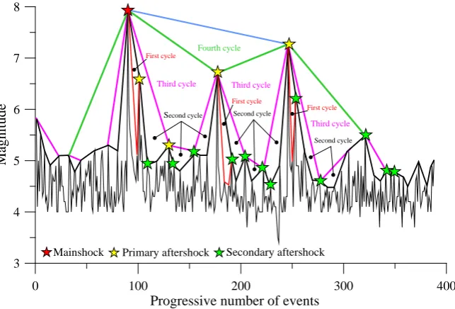
Figure 1. Schematic representation of Nepal earthquake’s aftershocks phase and after-shocks classification. The colored lines indicate the afterafter-shocks cycles.
Figure 2. Schematic representation of Nepal earthquake’s aftershocks phase and
after-shocks classification. The colored lines indicate the afterafter-shocks cycles.
1)Primary or direct aftershocks, which are triggered only by the mainshock (their time of occurrence and magnitude depend on the variations of stress generated by mainshock).
2)Secondary or indirect aftershocks, which are produced by stress variations re-lated to primary aftershocks. They occur after a primary aftershock, and are not directly connected to the original mainshock.
The time elapsed between the first primary aftershock and mainshock may
0 100 200 300 400
Progressive number of events 3
4 5 6 7 8
M
ag
n
it
u
d
e
Third cycle
Mainshock Primary aftershock Secondary aftershock
Fourth cycle
Third cycle
Third cycle Second cycle Second cycle
Second cycle First cycle
First cycle First cycle
0 100 200 300 400
Progressive number of events 3
4 5 6 7 8
M
ag
n
it
u
d
e
7.8 Mw 25/04/15
7.3 Mw 12/05/15 6.7 Mw
26/04/15
5.5 Mw 16/05/15
Mainshock Primary aftershock
Data Range: 24/07/09 to 26/11/15 Latitude: 32N - 26N Longitude: 80.5E - 88.5E Depth Range: 1-50 km Magnitude Range: 2.5-10.0 Catalog used: USGS Seismic sequence
NEPAL EARTHQUAKE
1
2
3
4
1
1
2
2
3
Secondary aftershock
1
1 2
1
2 1 2
[image:4.595.213.535.72.290.2] [image:4.595.210.538.337.587.2]vary, but typically it consists of a few hours/days, while the subsequent second-ary ones may happen in different areas and times.
From Figure 1, which shows the scheme of the aftershocks phase’s develop-mental structure triggered after the Nepal earthquake on 25/04/15 that was ob-tained by analyzing its branched structure [40], we can infer that in the seismic sequence a succession of cyclical movements (seismic cycles) was triggered, whose amplitude varies over time and with increasing magnitude and order. Here, any events occur following a specific hierarchisation process where each earthquake can generate other earthquakes [41].
These seismic events are connected to the event source and are considered as primary [42]. They may also, in turn, generate other minor seismic events, thus triggering a process which continues up to the energy release phase’s triggering point and may end with a major event.
The distribution of the most energetic aftershocks that close the sequence’s seismic cycles is usually repetitive and consists of a first primary aftershock si-tuated in time and space next to the mainshock, followed by a succession of lower magnitude secondary aftershocks and additional primary and secondary aftershocks.
Based on aftershocks time position with respect to mainshock, we obtain the development scheme and classification of the aftershocks shown in Figure 2, where we can observe that big events trigger a seismic events sequence consist-ing of several primary aftershocks of various order followed by secondary after-shocks of various orders, triggered by the previous ones.
Primary aftershocks may be of various order depending on the branched structure as well as aftershocks sequence’s developmental state. The magnitude values of primary aftershocks tend to grow from the third order onwards.
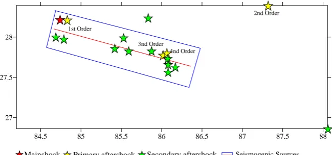
Figure 3 and Table 1 report the spatial distribution of primary and secondary
aftershocks’ seismic sequence that developed after the earthquake occurred in Nepal on 25 April 2015.
We observe that some aftershocks occurred in the co-seismic rupture area while others happened on the same fault, but outside the co-seismic rupture area
Figure 3. Schematic representation of epicenters of Nepal earthquake occurred on 25
April 2015 and relevant primary and secondary aftershocks.
84.5 85 85.5 86 86.5 87 87.5 88
27 27.5 28
1st Order
2nd Order
3nd Order 4nd Order
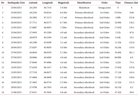
[image:5.595.211.536.545.697.2]Table 1. Primary and secondary aftershocks.
No Earthquake Date Latitude Longitude Magnitude Identification Order Time Distance (km)
1 25/04/2015 28.2305 84.7314 7.8 Mw Mainshock Sourge point 0 0
2 25/04/2015 28.2244 84.8216 6.6 Mw Primary aftershock 1st Order 33.93m 8.86
3 25/04/2015 28.3902 87.3173 5.7 mb Primary aftershock 2nd Order 3.09h 253.8
4 26/04/2015 27.7711 86.0173 6.7 Mw Primary aftershock 3nd Order 24.96h 136.2
5 12/05/2015 27.8087 86.0655 7.3Mw Primary aftershock 4nd Order 17.03d 139.1
6 25/04/2015 27.9945 85.5209 4.9 mb Secondary aftershock 1st Order 3.31h 87.8
7 25/04/2015 28.0979 84.5594 5.2 mb Secondary aftershock 2nd Order 6.54h 19.2
8 25/04/2015 28.2380 85.8290 5.1 mb Secondary aftershock 1st Order 11.52h 122.0
9 26/04/2015 27.8297 85.8650 5.0 Mw Secondary aftershock 1st Order 34.24h 119.9
10 27/04/2015 26.8644 88.0550 5.1 Mw Secondary aftershock 2nd Order 54.40h 361.1
11 27/04/2015 28.0066 84.6820 4.8 mb Secondary aftershock 2nd Order 60.80h 6.0
12 29/04/2015 27.8640 85.4086 4.6 mb Secondary aftershock 1st Order 4.22d 75.4
13 12/05/2015 27.6250 86.1617 6.3 Mw Secondary aftershock 1st Order 17.05d 155.8
14 12/05/2015 27.7318 86.0672 4.6 mb Secondary aftershock 2nd Order 17.12d 142.4
15 12/05/2015 27.6606 86.0849 4.5 mb Secondary aftershock 1st Order 17.14d 150.6
16 16/05/2015 27.5603 86.0734 5.5 Mw Secondary aftershock 3nd Order 21.22d 151.5
17 29/05/2015 27.9798 84.7819 4.8 mb Secondary aftershock 2nd Order 34.15d 6.2
18 11/06/2015 27.8321 85.5836 4.8 mb Secondary aftershock 1st Order 47.42d 94.8
while others, triggered by different earthquakes, occurred elsewhere, on faults adjacent to mainshock’s.
Aftershocks are distributed over a length of 150 km and a width of 70 km, in an easterly direction from the epicenter. One of them, with a 6.6 Mw magnitude (primary second order aftershock) occurred thirty minutes after the mainshock and in the epicentral area. On 12 May, a great Mw 7.3 magnitude aftershock (fourth order aftershock) occurred in the same location as the 25 April main-shock.
This spatial organization, suggests that the seismic rupture initiated on 25 April epicenter spread SE over more than a hundred kilometers, thus showing a SE-oriented stress switching, which probably triggered the 7.3 Mw event that closed the fifth order aftershocks cycle.
Aftershocks’ spatial organization is closely related to any energetic events oc-cured in the aftershocks phase. Immediately after the mainshock, most of the af-tershocks are located near or in close proximity to the mainshock’s rupture plane. Then, in many cases, the aftershocks migrate away from the mainshock, at a speed of 1 km/h up to 1 km/year calculated with reference to the mainshock or the first aftershock of first order.
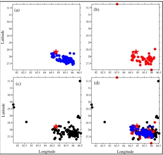
Figure 4 shows the distribution of aftershocks epicenters (USGS data) in the
Figure 4. Aftershocks phase in the Nepal earthquake on 25 April 2015. The red stars in-dicate the mainshock. For a detailed description, see the text.
tribution along the epicenters’ NW-SE direction before the occurrence of the first primary aftershock and an extension in SW-NE direction, with likely in-volvement of other faults after the first primary aftershock.
In particular, Figure 4(a) shows the SE spread of the aftershocks, from the mainshock to the first aftershock of first order. Figure 4(b) shows the after-shocks epicenters from the first aftershock of first order to the primary second order aftershock, in which we observe a shocks’ SW-NE extension. Figure 4(c), which starts from the first aftershock of first order on 19/11/15, we note a sub-sequent NE -NW aftershocks’ extension. Figure 4(d) shows the combination in time and space (aftershocks expansion and migration) from mainshock on 19/11/15.
In summary, the chart confirms an aftershocks extension in space and in time which is common to any aftershocks sequences.
The extent of aftershocks’ area extension or migration depends on the posi-tion of mainshock and primary most energetic shocks in the aftershocks phase.
Figure 5 and Figure 6 display some reports drafted using 86 primary
after-shocks occurred in various areas of the world and recorded by INGV, NIED AND USGS networks between 1970 and 2016.
Figure 5(a) shows the existing relationship between the number of days
elapsed between the mainshock and the most energetic primary aftershock and the aftershock magnitude, while Figure 5(b) shows the relation between the dis-
82 82.5 83 83.5 84 84.5 85 85.5 86 86.5
Longitude 27.5
28 28.5 29 29.5 30 30.5 31 31.5
L
at
it
u
d
e
82 82.5 83 83.5 84 84.5 85 85.5 86 86.5
27.5 28 28.5 29 29.5 30 30.5 31 31.5
82 82.5 83 83.5 84 84.5 85 85.5 86 86.5
27.5 28 28.5 29 29.5 30 30.5 31 31.5
L
at
it
u
d
e
82 82.5 83 83.5 84 84.5 85 85.5 86 86.5
Longitude 27.5
28 28.5 29 29.5 30 30.5 31 31.5
(a) (b)
Figure 5. (a) Relationship between the number of days elapsed between mainshock and the most energetic primary aftershock (abscissa) and the aftershock magnitude (ordi-nate); (b) Relationship between the distance in kilometers between the mainshock and the most energetic primary aftershock (abscissa) and the aftershock magnitude (ordinate).
Figure 6. (a) Relationship between the aftershock’s occurrence time from mainshock
(abscissa) and the distance between the mainshock (ordinate); (b) Relationship between the mainshock and the most energetic primary aftershock magnitudes.
tance in kilometers between the mainshock and the most energetic primary af-tershock and the afaf-tershock magnitude.
In general, our analyses show that in seismic sequences the aftershocks phase tends to develop within seconds, days and years and with a spatial development initially next to the mainshock epicenter, which causes their triggering. Subse-quently, they are organized into placed bands at different distances, even of 100 km. The main aftershock’s incidence mostly occurs at a distance of 0 - 50 km.
The frequency of the aftershocks that occur within 24 hours after the mashock, decreases as the days increase, while aftershocks magnitude values in-crease as the distance inin-creases.
The percentage of aftershocks that occur within 24 hours after the mainshock is 63%, while for those that occur at less than 50 km is 70%.
Figure 6(a) shows the relationship between the number of days elapsed from
(b) (a)
(b) (a)
5 6 7 8 9
Magnitude of mainshock (Mw) 4
5 6 7 8 9
M
ag
n
it
u
d
e
o
f
af
te
rs
h
o
ck
(
M
w
)
b) N = 86
MA = 0.482MM + 2.564
r2 = 0.293
0 4 8 12 16 20
Time (Day) 0
100 200 300
D
is
ta
n
ce
o
f
m
ai
n
sh
o
ck
(
k
m
)
a)
[image:8.595.212.535.310.480.2]the mainshock and the distance between the mainshock and the most energetic primary aftershock. The figure shows that many aftershocks occur less than one day away from mainshock and within 50 km. The aftershocks frequency de-creases as both distance (up to hundreds of kilometers) and time (up to ap-proximately 18 days) increase.
Figure 6(b) shows the relationship between the mainshock magnitude and
the most energetic primary aftershock, which is valid for any area in the world and can be used to assess an aftershock magnitude.
The average aftershock magnitude value (Mf) is calculated using the following empirical relationship, obtained by the graph displayed in Figure 6(d):
0.482 2.564
A M
M = M + (1)
3. Methods for Identifying Aftershocks
3.1. Branched Structure
After the occurrence of a strong earthquake, in order to study the future devel-opment of the seismic sequence, it is crucial to know how aftershocks develop, in particular the value of their magnitude and their type (primary and secondary). The aftershocks occurrence may indicate a greater seismic hazard of the area in the short time following the mainshock.
A simple and effective method to monitor aftershocks evolution, and to iden-tify the most energetic ones, is based on the seismic sequence time hierarchisa-tion process [40], where a primary or secondary aftershock of various order can be described by a branched structure originating from the mainshock.
This procedure allows distinguishing the aftershocks directly triggered by the mainshock from those triggered by other second generation higher order shocks. The method has been tested on various catalogs with good results since after-shocks are easier to define compared to foreafter-shocks.
Figure 7 shows branched structures of various orders that were formed after
the Solomon Island earthquake on 21 April 1977 (point source) and primary and secondary aftershocks of various order located at the seismic nodes of branched structures’ branches.
Primary and secondary aftershocks are distinguished by their magnitude-de- pendent position in the aftershocks sequence and by the connections, both direct and indirect, with the mainshock.
Primary aftershocks are triggered by the mainshock, while the secondary, over the time, are triggered by primary aftershocks-induced stress variations.
Thus, a shock could be an aftershock linked either to the mainshock or to one of the previous aftershocks and, at the same time, to the most energetic shock of subsequent aftershocks.
Figure 7. Branched structure of Solomon Island earthquake on 21 April 1977.
The aftershocks development’s overall scheme can provide useful information about the future sequence development and the likely occurrence of major events.
3.2. Use of Relative Maximum and Minimum Magnitude Values
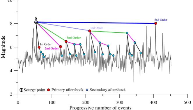
The graphic approach proposed is based on mainshock magnitude values and relative maximum and minimum values that are formed during the aftershocks sequence’s time evolution. The graphic procedure allows forecasting the devel-opment of the most energetic aftershocks that occur immediately after the mainshock or a primary aftershock and assessing their magnitude.Figure 8 shows the procedure suited to identify the first relative minimum
value that is formed after the mainshock and that allows determining even the beginning of the second seismic cycle in the post-earthquake energy release.
The first step consists in identifying the midpoint (Point 3) of the line joining the mainshock (Point 1) with the minimum value that precedes it (Point 2). From point 2 a horizontal line must be drawn util it intrersects the straight ver-tical line (Point 4) crossing the most energetic event (Point 1) and this intersec-tion must be joined with the midpoint (Point 3). From point 1 we draw a line parallel to the line crossing points 3 and 4, thus establishing the channel in which magnitude values fluctuations will develop during the first post-earth- quake phase.
Figure 9 shows the procedure suited to detect the most energetic aftershocks
directly triggered by the main earthquake or by a primary aftershock and the band in which the magnitude values fluctuations will develop.
From the mid-point we draw an half line crossing the minimum value (Point 1) indicated by the broken line of the relative maximum and minimum values and by the mainshock, then we draw the parallel line whose slope will provide the magnitude value at the first aftershock occurrence point (Point 2).
It is necessary to repeat the same procedure for identifying the position and
0 100 200 300 400 500
Progressive number of events
2 4 6 8 10
M
ag
n
it
u
d
e
2nd Order
3nd Order
4nd Order
1st Order
S 5nd Order
Figure 8. Procedure for determining the first minimum value of the relative maximum and minimum values line. The red star indicates the Nepal earthquake on 25 April 2015, the yellow stars the most energetic aftershocks. The red circles indicate the aftershocks magnitude values in the post-seismic phase.
Figure 9. Procedure for determining primary and secondary aftershocks. The red star
in-dicates the Nepal earthquake on 25 April 2015, the yellow stars indicate the most ener-getic aftershocks. The red and blue lines show the aftershocks magnitude values fluctua-tions range.
the magnitude value of other expected aftershocks (4, 8, 12). It is possibile to implement the same procedure from the most energetic aftershocks and from point M1 to obtain the magnitude values fluctuation range of the aftershock ex-pected. For example, from midpoint A1 it is possible to identify Point 11 using
0 100 200 300 400
Progressive number of events
3 4 5 6 7 8
M
ag
n
it
u
d
e
7.8 Mw
7.3 Mw
6.7 Mw
5.5 Mw 25-04-15
26-04-15
12-05-15
16-05-15 5
6
7
1
2
3
4
0 100 200 300 400
Progressive number of events
3 4 5 6 7 8
M
ag
n
it
u
d
e
7.8 Mw
6.7 Mw 25-04-15
M1 A
A1
1 2
3 4
5 7
8
10 11 9
M
12
[image:11.595.212.536.371.604.2]the same procedure and compare it with Point 12 previously identified from point A.
[image:12.595.215.537.478.704.2]This procedure identifies the channel where future aftershock’ possible fluc-tuations will occur, when it is formed, after a relative minimum value (Point 5), a temporary relative maximum value (Point 6), also identifying the most ener-getic one. This method has proved to be very effective, although, from the study of some seismic sequences, we infer that in the energy release phase the values identified through the graphic method are not always respected.
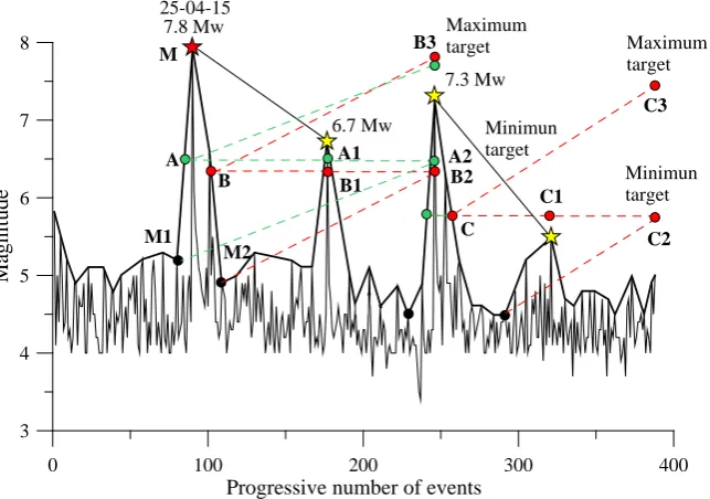
Figure 10 shows the graphic procedure for estimating the expected magnitude
values (magnitude target) of primary and secondary aftershocks, depending on the position of relative maximum and minimum values points in respect to the midpoint of the energy accumulation and release phases (seismic cycles), which are triggered in the seismic sequence.
Operationally, for the calculation of an aftershock minimum magnitude target it is sufficient to calculate the value of the midpoint B between the relative min-imum M2 and the mainshock. The maxmin-imum value is obtained by drawing a line from midpoint M2 up to the calculation point selected (Point B2) and join this with the relative minimum M2 (dashed red line). We then d draw from the mid-point B a line parallel to M2-B2, where the point B3 represents the maxi-mum magnitude value expected. The same procedure can be repeated from midpoint A or from other energetic aftershocks to detect the position of the maximum and minimum magnitude value of other aftershocks expected (Points C2 and C3).
3.3. Index Simplified Force (ISF)
Index Simplified Force ISF is a very simple and sensitive oscillator, which can be
Figure 10. Procedure for determining the magnitude value of primary and secondary
af-tershocks.
0 100 200 300 400
Progressive number of events
3 4 5 6 7 8
M
ag
n
it
u
d
e
7.8 Mw
6.7 Mw 25-04-15
A B
7.3 Mw
Minimun target Maximum target Maximum
target
M
M1
M2
A1
B1 B2
B3
A2
Minimun target
C
C1
used to monitor the seismic sequence strength and the relevant development
[43] and to control the aftershocks phase.
The ISF overall decay rate is similar to the decay rate of a generic aftershocks sequence.
[image:13.595.211.536.295.693.2]Moreover, the greater the magnitude of the mainshock the steeper the power decay law (more similar to an exponential decay).
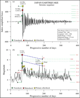
Figure 11 shows the Japan seismic sequence in the time window ranging from
2 January to 31 December 2011, the ISF and simplified Aroon oscillator [40].
Figure 11(a) shows, up to 8 March 2011, an initial portion of small amplitude
cyclical fluctuations, followed, on 9 March, by a first peak due to the occurrence of a magnitude 7.3 Mw foreshock (green star) associated with an increase in the number of recorded events and shortly afterwards by a ISF second increase due to the mainshock, whose magnitude was 9.0 Mw (red star), occurred on the same day. A third peak of greater amplitude formed on 13 March with the af-
Figure 11. (a) Index Simplified Force in the 2011 Japan earthquake’s seismic sequence;
(b) Daily seismic sequence. On the right, red-colored Fibonacci levels 0% - 100% are shown.
0 100 200 300 400
Progressive number of days -800 -400 0 400 800 In d ex s im p li fi ed f o rc e Seismic sequence JAPAN EARTHQUAKE 9.0 Mw 11/03/11 Foreshock Mainshock 7.3 Mw 09/03/11 Aftershock 6.6 Mw 13/03/11
Data Range: 02/01/11 to 31/12/11 Latitude: 42N - 30N Longitude: 145E - 130E Depth Range: 1-50 km Magnitude Range: 2.5-10.0 Catalog used: NIED
0 100 200 300 400
Progressive number of days 2 4 6 8 10 M ag n it u d e 7.3 Mw 10/07/11 4nd Order
Foreshock Mainshock Primary aftershock
2 3 . 6
3 8 . 2
5 0 . 0
6 1 . 8
7 6 . 4
1 0 0 . 0 0 . 0
2 3 .6
3 8 .2
5 0 .0
6 1 .8
7 6 .4
1 0 0 .0 0 .0
a)
b) 9.0 Mw
tershock occurrence, with a magnitude of 6.6 Mw (yellow star) associated with a sharp increase in the number of daily events recorded. After the aftershock on 13 March, the ISF values decreased over time and, at the end of December, reached values similar to pre-foreshock’s on 9 March 2011.
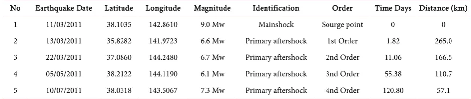
Table 2 reports the most energetic aftershocks closing the seismic cycles that
developed in the daily sequence of aftershocks during Japan earthquake in 2011. Inside the aftershocks sequence we find some seismic levels where magnitude values, during their post-earthquake fluctuation, more frequently stop, which offer some useful information for estimating the magnitude values that might occur in future.
The seismic levels used in this work, which give information on the aftershock sequence’s developmental state are Fibonacci levels [44].
The levels are 23.6%, 38.2%, 50%, 61.8%, 76.4% and 100%, respectively.
Figure 11(a) and Figure 11(b) show ISF and seismic sequence percentage
le-vels, i.e. the static seismic levels.
The procedure adopted consists in identifying in the seismic sequence or ISF chart the previous maximum (Level A) and minimum value (B) from which the maximum value is derived and then dividing the distance between the minimum and maximum values by carrying Fibonacci percentage levels (green dashed ho-rizontal lines).
The graph thus created provides the following information:
• The most energetic post-seismic phase usually ends as the magnitude values
are set under the seismic level-static of 50%;
• The highest occurrence frequency of the most energetic aftershocks occurs in
the seismic level range between 23.6% and 50%;
• The occurrence and the magnitude value of the first primary aftershock
ex-pected after the mainshock depend on the first minimum level (C) that is formed after the main event. The lower the distance of the seismic level C from maximum value A, the greater the magnitude of the first primary after-shock (usually the subsequent magnitude increase from seismic level C, does not exceed 50% of the magnitude difference between maximum value A and seismic level C);
• The aftershocks sequence starts at the end of the process, when magnitude
values are set under the background seismicity maximum value (D) which usually coincides with seismic levels of 61.8% and 76.4% (with greater fre-quency), respectively.
Table 2. Primary aftershocks phase in the Japan earthquake.
No Earthquake Date Latitude Longitude Magnitude Identification Order Time Days Distance (km)
1 11/03/2011 38.1035 142.8610 9.0 Mw Mainshock Sourge point 0 0
2 13/03/2011 35.8282 141.9723 6.6 Mw Primary aftershock 1st Order 1.82 265.0
3 22/03/2011 37.0860 144.2480 6.7 Mw Primary aftershock 2nd Order 11.06 166.5
4 05/05/2011 38.2122 144.1190 6.1 Mw Primary aftershock 3nd Order 55.38 110.7
To know in advance the magnitude values range of the most energetic after-shocks sequence, it is possible to use a quite simple and fast graphic method, which consists in building a dynamic seismic level by combining the maximum value (main event) with the end of the 14.6% seismic level selected for the calcu-lation (Point E1). From the left end of the 23.6% seismic level we draw a parallel line to the previously plotted dynamic level in order to identify Point E2.
The range between the dynamic seismic levels’ ends (Points E1 and E2) represents the preliminary range of magnitude values of higher order most energetic aftershocks.
Figure 12 shows the relationship between the number of daily events and ISF
(all values were considered positive) and between the daily magnitude (maxi-mum value recorded during the day) of aftershocks and IFS.
The graph displayed in Figure 12(a) was built by plotting the highest ISF val-ue (point A) which usually coincides with the day of the mainshock or a subse-quent more energetic aftershock, and joining this point with the origin of the axes (0,0). Subsequent ISF values are progressively arranged along this segment from Point A to the origin of the axes.
The segment represents a trend line expressing the temporal behavior of the aftershocks sequence through ISF.
The ISF chart seems to follow a linear pattern that allows predicting the after-shocks phase evolution and end. In fact, when the ISF values begin to cluster near the axes’ origins, it means that the aftershocks phase is about to be com-pleted. In the graph shown in Figure 12(b), the IFS features a logarithm trend with very dispersed values around the average value, representing a source of uncertainty in the relationship between the daily maximum magnitude and ISF.
Figure 13 shows some reports that can provide useful information on
after-shock sequence development.
Figure 13(a) and Figure 13(b) shows the time trends in the number of daily
Figure 12. (a) Relationship between daily number of earthquakes and ISF. The black line
is the interpolating line, while the red line is the trend line of the aftershocks sequence provided. The green circle shows the greatest ISF value; (b) Relationship between the dai-ly maximum magnitude and ISF.
[image:15.595.211.537.504.678.2]Figure 13. (a) Relationship between the progressive number of days and the number of daily events; (b) Relationship between the progressive number of days and magnitude values; (c) Relationship between the progressive number of days and ISF; (d) Relationship between the progressive number of events and ISF in energy accumulation and release phases. The green and red circles indicate the greatest ISF value in the energy accumula-tion and release phases.
events and magnitude values, while Figure 13(c) displays the ISF temporal trend. The latter figure shows that an exponential decay prevails in the very short term, while a linear ISF decay is dominant in the long term.
Figure 13(d) reports the relationship between the number of daily events and
ISF values in relation to energy accumulation and release phases. By default, we assumed that the energy accumulation earthquakes have a lower magnitude val-ue compared to the previous one, while if the magnitude valval-ue is greater than the previous earthquake, they are considered as release energy earthquakes.
The energy accumulation and release phases originating from ISF maximum values show that energy accumulation shocks outnumbered the energy release phase’s and that the energy accumulation phase was stronger shortly after the mainshock (ISF values are greater and closer to the point of origin (B).
This graph allows evaluating the aftershocks phase development and estimat-ing systematically the ISF value through the followestimat-ing relation:
(
)
ISF=0.5 ISF++ISF− (2)
where,
ISF* is the index of the energy release phase strength (ISF > 0).
0 100 200 300 400
Progressive number of days 0 40 80 120 N u m b er o f d ai ly e v en ts
0 100 200 300 400
Progressive number of days 2 4 6 8 10 M ag n it u d e
0 100 200 300 400
Progressive number of days -800 -400 0 400 800 IS F
0 40 80 120
ISF− is the index of the energy accumulation phase strength (ISF < 0).
The ISF+ and ISF− values can be obtained from the ISF decay curves displayed
in Figure 13(c) or from Figure 13(d).
[image:17.595.234.511.310.689.2]Besides, in order to predict when the most energetic energy release phase will end, Figure 13(d) shows a simple graphic procedure based on the energy accu-mulation phase’s IFS-value. The procedure is as follows: on the positive ordinate axis the ISF maximum value related to the energy accumulation phase is re-ported (Point C). From this, a line is plotted (dashed red line) in parallel with the line joining the origin with Point B. Intersection point D between this paral-lel line and the line joining the origin with the point A, separates the phase in which the most energetic aftershocks occur (IFS+ values greater than D) from the least energetic one (IFS+ values smaller than D).
Figure 14 shows the relationship between the number of daily events and ISF
in relation to some earthquakes occurred in Italy, Gulf of Alaska, Sumatra and Japan.
Figure 14. Relationship between the number of daily events and ISF of the following
earthquakes: (a) Gulf of Alaska of 30/11/1987; (b) Sumatra on 26/12/2004; (c) Japan 11/03/2011; (d) L’Aquila 06/04/2009; (e) Emilia 20/05/2012; (f) Central Italy, 30/10/2016.
0 10 20 30 40
Number of daily events -200 -100 0 100 200 300 IS F
a) Gulf of A laska
0 100 200 300 400
Number of daily events -1000 0 1000 2000 IS F
f) Central Italy
0 40 80 120
Number of daily events -800 -400 0 400 800 IS F c) Japan B B B A A A
0 40 80 120 160 200
Number of daily events -1000 -500 0 500 1000 1500 IS F B A b) Sumatra
0 100 200 300 400
Number of daily events -1000 0 1000 2000 IS F 7.9 Mw 7.0 Mw 6.6 Mw 9.0 Mw 5.2 Mw 9.1 Mw 8.6 Mw 6.5 Mw 5.5 Mw 4.8 Mw 4.7 Mw 5.8 Mw 5.6 Mw 3.8 Mw
0 200 400 600 800
Number of daily events -2000 0 2000 4000 6000 IS F 5.9 Mw 5.4 Mw 5.0 Mw A A B B
d) L 'A quila
e) Emilia 6.7 Mw 4.7 Mw 3.8 Mw D D D D D 5.9 Mw 6.1 Mw 4.1 Mw
3.8 Mw 4.2 Mw
6.2 Mw 5.6 ML
The aftershocks phase can be monitored through the branched structure as well.
Figure 15 presents ISF hierarchisation process in relation to four primary
values of various orders. Simplified Aroon oscillator allows monitoring the trend and identifying the warning signs that precede the highest ISF values.
Usually the first primary point of first order closes the most energetic post-seismic phase, while the closure of the most energetic aftershocks starts from the primary point of higher order with the greatest frequency.
3.4. Numerical Method to Calculate Aftershock’s Magnitude
Knowing the magnitude value of the most energetic aftershock that follows a mainshock is crucial to study the sequence’s time evolution and obtain informa-tion on possible major earthquakes in the future.
The empirical Båth law [45] states that the average difference in magnitude between a mainshock and the most energetic aftershock is 1.2 (Δm), indepen-dently of the mainshock magnitude.
Subsequent studies have confirmed the Båth’s law statement, but have pro-vided Δm values in the 0 - 3 range [2] [46].
Figure 16 shows the empirical relations valid for any area in the world that
allow us to estimate an aftershock magnitude knowing mainshock or after-shocks’ previously occurred.
[image:18.595.212.532.417.719.2]The report shown in Figure 16(a) was obtained from the study of primary
Figure 15. ISF hierarchisation. Under the ISF chart is the simplified Aroon oscillator.
0 100 200 300 400
Progressive number of days
-800 -400 0 400 800
In
d
e
x
s
im
p
li
fi
e
d
f
o
rc
e
Seismic sequence
JAPAN EARTHQUAKE
9.0 Mw 11/03/11
Foreshock Mainshock
7.3 Mw 09/03/11
Aftershock 6.6 Mw
13/03/11
Primary ISF
4nd Order
3nd Order 3nd Order
1st Order
80
50
Figure 16. Relationship between mainshock and the most energetic aftershocks.
and secondary aftershocks whose order was greater than M > 3.6, recorded by INGV, NIED AND USGS seismic networks between 1970 and 2016.
0.942 0.128
A M
M = M − (3)
where MM is the magnitude value of the mainshock or of a subsequent, more energetic aftershock.
The empirical report points out that an aftershock magnitude is, on average, 0.484 (Δm) smaller than the mainshock or aftershock which it depends on and suggests a certain degree of self-similarity to the earthquake that has triggered it.
Figure 16(b) shows the relationship between the mainshock magnitude and
the most energetic aftershock’s recorded within ten days after the mainshock occurrence and in an area of 50 km around the mainshock epicenter.
The aftershock average magnitude value (MA) is calculated by the following relation obtained from the analysis of 55 strong earthquakes occurred in various areas of the world:
0.631 1.419
A M
M = M + (4)
The average difference in size between the mainshock and the most energetic aftershock is 1.287 (Δm), which is slightly higher than that obtained by the em-pirical Båth’s law.
Figure 17 shows the relationship between the mainshock magnitude and the
most energetic aftershock’s recorded within twenty-four hours after the main-shock.
The aftershock average magnitude value (MA) is estimated by the following relation obtained from the analysis of 128 strong earthquakes occurred in vari-ous areas of the world:
0.771 0.0661
A M
M = M + (5) The average difference in size between the mainshock and the most energetic aftershock is 1.575 (Δm).
4. Conclusions
Any mainshock is generally followed by a series of aftershocks, whose duration
2 4 6 8 10
Magnitude mainshock/aftershock 2
4 6 8 10
M
ag
n
it
u
d
e
af
te
rs
h
o
ck
5 6 7 8 9
Magnitude mainshock 4
5 6 7 8
M
ag
n
it
u
d
e
af
te
rs
h
o
ck
b) N=55
MA = 0.631 MM + 1.419 r2=0.431
σ=0.235 a)
N=204
MA = 0.942 MM - 0.128 r2=0.894
σ=0.114
Figure 17. Relationship between the most energetic mainshocks and aftershocks.
may vary from a few weeks to several months or years.
Aftershocks typically give birth to a series of primary and secondary after-shocks of different orders whose magnitude is lower compared to the main event’s, which can be identified through a sequence hierarchisation process. The primary aftershocks result from a triggering process due to mainshock-induced stress variation, and the secondary aftershocks are triggered by stress changes occurred in primary aftershocks.
During our analyses:
• we have created an empirical relation valid for any area in the world, to
esti-mate an aftershock’s magnitude knowing that of a mainshock or a previous aftershock;
• we have observed that some aftershocks occur along the same fault that has
generated the mainshock, or outside the area where the seismic sequence de-velops and additional aftershocks can occur on adjacent faults;
• based on a graphic procedure applied using the seismic sequence’s relative
maximum and minimum values, we obtained useful information for predict-ing the most energetic aftershocks and assesspredict-ing their magnitude;
• we suggested the use of the index simplified force-ISF in combination with
Fibonacci levels, which allows predicting an aftershocks sequence’s time evo-lution and then the developmental state reached by the seismic sequence;
• we determined the relationship between the mainshock’s magnitude and the
most energetic aftershock’s recorded within ten days of the mainshock occur-rence and within an area of 50 km around the mainshock epicenter;
• between the mainshock’s magnitude and the most energetic aftershock’s
rec-orded within twenty-four hours after the mainshock, we have provided an av-erage magnitude difference of 1.287 and 1.575, respectively, which is slightly higher than that obtained with the empirical Båth’s law.
This method allows us to monitor an aftershock development in the short- medium term, providing useful insights into its future development. As some of
5 6 7 8 9 10
Magnitude mainshock
3 4 5 6 7 8
M
ag
n
it
u
d
e
af
te
rs
h
o
ck
N=128
MA = 0.771 MM + 0.0661 r2=0.450
the aforementioned procedures show no close mainshock-aftershock relations, we believe that they deserve further in-depth investigations in order to obtain an even more effective forecasting model.
References
[1] Doglioni, C., Barba, S., Carminati, E. and Riguzzi, F. (2014) Fault On-Off versus Strain Rate and Earthquakes Energy. Geoscience Frontiers, 6, 265-276.
[2] Felzer, K.R., Thorsten, W., Becker, T.W., Abercrombie, R.E., Ekström, G. and Rice, J.R. (2002) Triggering of the 1999 Mw 7.1 Hector Mine Earthquake by Aftershocks
of the 1992 Mw 7.3 Landers Earthquake. Journal of Geophysical Research, 107, 2190.
https://doi.org/10.1029/2001JB000911
[3] Kisslinger, C. (1996) Aftershocks and Fault-Zone Properties. In: Advances in Geo-physics, Vol. 38, Academic Press, Inc., Cambridge, MA.
[4] Lay, T. and Wallace, T. (1995) Modern Global Seismology. Academic Press, Inc., Cambridge, MA, 521 p.
[5] Nur, A. and Booker, J. (1972) Aftershocks Caused by Pore Fluid Flow? Science, 175, 885-887. http://science.sciencemag.org/content/175/4024/885
https://doi.org/10.1126/science.175.4024.885
[6] Main, I. (2006) Earthquakes: A Hand on the Aftershock Trigger. Nature, 441, 704- 705. https://doi.org/10.1038/441704a
[7] Van der Elst, N. J. and Brodsky, E.E. (2010) Connecting Near-Field and Far-Field Earthquake Triggering to Dynamic Strain. Journal of Geophysical Research, 115, B07311. https://doi.org/10.1029/2009JB006681
[8] King, G.C.P., Stein, R.S. and Lin, J. (1994) Static Stress Changes and the Triggering of Earthquakes. Bulletin of the Seismological Society of America, 84, 935-953. [9] Belardinelli, M.E., Bizzarri, A. and Cocco, M. (2003) Earthquake Triggering by
Stat-ic and DynamStat-ic Stress Changes. Journal of Geophysical Research, 108, 2135. https://doi.org/10.1029/2002jb001779
[10] Scholz, C.H. (2002) The Mechanics of Earthquakes and Faulting. 2nd Edition, Cambridge University Press, Cambridge.
https://doi.org/10.1017/cbo9780511818516
[11] Omori, F. (1894) Investigation of Aftershocks. Reports of the Imperial Earthquake Investigation Committee,, 2, 103-139.
[12] Marcellini, A. (1997) Physical Model of Aftershock Temporal Behaviour. Tectono-physics, 277, 137-146.
[13] Utsu, T. (1971) Aftershocks and Earthquake Statistics (III). Journal of the Faculty of Science, Hokkaido University. Series 7, Geophysics, 3, 379-441.
[14] Scholz, C.H. (1972) Crustal Movements in Tectonic Areas. Tectonophysics, 14, 201- 217.
[15] Yamanaka, Y. and Shimazaki, K. (1990) Scaling Relationship between the Number of Aftershocks and the Size of the Main Shock. Journal of Physics of the Earth, 38, 305-324. https://doi.org/10.4294/jpe1952.38.305
[16] Mendoza, C. and Hartzell, S.H. (1988) Aftershock Patterns and Mainshock Faulting. Bulletin of the Seismological Society of America, 78, 1438-1449.
Geophys. Mono. 37, American Geophysical Union, Washington DC, 195-207. https://doi.org/10.1029/gm037p0195
[18] Whitcomb, J., Allen, C., Garmany, J. and Hileman, J. (1973) San Fernando Earth-quake Series, 1971: Focal Mechanisms and Tectonics. Reviews of Geophysics, 11, 693-730. https://doi.org/10.1029/RG011i003p00693
[19] Mogi, K. (1969) Relationship between the Occurrence of Great Earthquakes and Tectonic Structures. Bulletin of the Earthquake Research Institute, University of Tokyo, 47, 429-441.
[20] Tajima, F. and Kanamori, H. (1985) Global Survey of Aftershock Area Expansion Patterns. Physics of the Earth and Planetary Interiors, 40, 77-124.
[21] Houghs, S.E. and Jones, L.M. (1997) Aftershocks: Are They Earthquakes or After-thoughts? EOS, Transactions American Geophysical Union, 78, 505-508.
https://doi.org/10.1029/97EO00306
[22] Helmstetter, A. and Sornette, D. (2003) Båth’s Law Derived from the Guten-berg-Richter Law and from Aftershocks Properties. Geophysical Research Letters, 30, 2069. https://doi.org/10.1029/2003GL018186
[23] Parsons, T. and Velasco, A.A. (2009) On Near-Source Earthquake Triggering. Journal of Geophysical Research, 114, B10307.
https://doi.org/10.1029/2008jb006277
[24] Gardner, J.K. and Knopoff, L. (1974) Is the Sequence of Earthquakes in South-ern-California, with Aftershocks Removed, Poissonian? Bulletin of the Seismologi-cal Society of America, 64, 1363.
[25] Keilis-Borok, V.I., Knopoff, L. and Rotwain, I.M. (1980) Bursts of Aftershocks, Long-Term Precursors of Strong Earthquakes. Nature (London), 283, 259-263. https://doi.org/10.1038/283259a0
[26] Reasenberg, P. (1985) Second-Order Moment of Central California Seismicity, 1969-1982. Journal of Geophysical Research, 90, 5479-5495.
https://doi.org/10.1029/JB090iB07p05479
[27] Davis, S.D. and Frohlich, C. (1991) Single-Link Cluster Analysis, Synthetic Earth-quake Catalogues, and Aftershock Identification. Geophysical Journal International, 104, 289-306. https://doi.org/10.1111/j.1365-246X.1991.tb02512.x
[28] Molchan, G.M. and Dmitrieva, O.E. (1992) Aftershock Identification: Methods and New Approaches. Geophysical Journal International, 109, 501-516.
https://doi.org/10.1111/j.1365-246X.1992.tb00113.x
[29] Zhuang, J., Ogata, Y. and Vere-Jones, D. (2002) Stochastic Declustering of Space- Time Earthquake Occurrences. Journal of the American Statistical Association, 97, 369-380. https://doi.org/10.1198/016214502760046925
[30] Zhuang, J., Ogata, Y. and Vere-Jones, D. (2004) Analyzing Earthquake Clustering Features by Using Stochastic Reconstruction. Journal of Geophysical Research, 109, B05301. https://doi.org/10.1029/2003jb002879
[31] Baiesi, M. and Paczuski, M. (2004) Scale-Free Networks of Earthquakes and After-shocks. Physical Review E, 69, Article ID: 066106.
https://doi.org/10.1103/PhysRevE.69.066106
[32] Baiesi, M. and Paczuski, M. (2005) Complex Networks of Earthquakes and After-shocks. Nonlinear Processes in Geophysics, 12, 1-11.
https://doi.org/10.5194/npg-12-1-2005
[34] Marsan, D. and Lengliné, O. (2008) Extending Earthquake’ Reach through Cascad-ing. Science, 319, 1076-1079. https://doi.org/10.1126/science.1148783
[35] Felzer, K. and Brodsky, E. (2006) Decay of Aftershock Density with Distance Indi-cates Triggering by Dynamic Stress. Nature, 441, 735-738.
http://www.nature.com/nature/journal/v441/n7094/abs/nature04799.html [36] Helmstetter, A. and Sornette, D. (2002) Diffusion of Epicenters of Earthquake
Af-tershocks, Omori’s Law and Generalized Continuous-Time Random Walk Models. Physical Review E, 66, Article ID: 061104.
https://journals.aps.org/pre/abstract/10.1103/PhysRevE.66.061104
[37] Mogi, K. (1968) Development of Aftershock Areas of Great Earthquakes. Bulletin of the Earthquake Research Institute, University of Tokyo, 46, 175-203.
http://repository.dl.itc.u-tokyo.ac.jp/dspace/handle/2261/12382
[38] Tajima, F. and Kanamori, H. (1985) Global Survey of Aftershock Area Expansion Patterns. Physics of the Earth and Planetary Interiors, 40, 77-134.
http://www.sciencedirect.com/science/article/pii/0031920185900664
[39] Valdés, C., Meyer, R., Zuniga, R., Havskov, J. and Singh, K.S. (1982) Analysis of the Petatlan Aftershocks: Numbers, Energy Release, and Asperities. Journal of Geo-physical Research, 87, 8519-8527.
http://onlinelibrary.wiley.com/doi/10.1029/JB087iB10p08519/full https://doi.org/10.1029/JB087iB10p08519
[40] Riga, G. and Balocchi, P. (2016) Short-Term Earthquake Forecast with the Seismic Sequence Hierarchization Method. Open Journal of Earthquake Research, 5, 79-96. https://doi.org/10.4236/ojer.2016.52006
[41] Marzocchi, W. and Lombardi, A.M. (2008) A Double Branching Model for Earth-quake Occurrence. Journal of Geophysical Research, 113, B08317.
https://doi.org/10.1029/2007JB005472
[42] Werner, M.J. (2008) On the Fluctuations of Seismicity and Uncertainties in Earth-quake Catalogs: Implications and Methods for Hypothesis Testing. Dissertation, University of California, Los Angeles.
https://www.ethz.ch/content/dam/ethz/special-interest/mtec/chair-of-entrepreneuri al-risks-dam/documents/dissertation/Max_Werner_thesis_final_Dec07.pdf [43] Riga, G. and Balocchi, P. (2017) How to Identify Foreshocks in Seismic Sequences
to Predict Strong Earthquakes. Open Journal of Earthquake Research, 6, 55-71. https://doi.org/10.4236/ojer.2017.61003
[44] Cohen, G. (2005) Options Made Easy, Your Guide to Profitable Trading, FT Pren-tice Hall. Pearson Education, Inc., London.
ftp://nozdr.ru/biblio/kolxo3/F/FD/FDtrd/Cohen%20G.%20Options%20Made%20Ea sy..%20Your%20Guide%20to%20Profitable%20Trading%20(2ed.,%20FTPH,%2020 05)(ISBN%200131871358)(369s)_FDtrd_.pdf
[45] Båth, M. (1965) Lateral in Homogeneities in the Upper Mantle. Tectonophysics, 2, 483-514.
Submit or recommend next manuscript to SCIRP and we will provide best service for you:
Accepting pre-submission inquiries through Email, Facebook, LinkedIn, Twitter, etc. A wide selection of journals (inclusive of 9 subjects, more than 200 journals)
Providing 24-hour high-quality service User-friendly online submission system Fair and swift peer-review system
Efficient typesetting and proofreading procedure
Display of the result of downloads and visits, as well as the number of cited articles Maximum dissemination of your research work