Semi Numerical Solution for a Boundary Value Problem
N. P. Pai1*, N. N. Katagi1, Krishna B. Chavaraddi2
1Department of Mathematics, Manipal Institute of Technology, Manipal University, Manipal, India 2Government First Grade College, Yellapur, India
Email: *[email protected], [email protected], [email protected] Received October 29, 2012; revised December 9, 2012; accepted December 22, 2012
ABSTRACT
The flow of viscous incompressible fluid through a tube is considered. The similarity transformation is used to reduce the governing equations into nonlinear ordinary differential equation. The solution procedure includes application of long series analysis with polynomial coefficients. The series representing physical parameters ( f
1 , f
1 ) reveal qualitative features which are comparable to pure numerical results. The analysis enables in extending region of validity. A complete description of the solutions is presented.Keywords: Computer Extended Series; Domb-Sykes Plot; Pade’ Approximants; Polynomial Coefficients
1. Introduction
Unsteady flows produced by a simple contraction or ex-pansion of the wall have wide applications, for example, in physiological pumps, peristaltic motion Jafrin [1] pro- blems involving collapsible tubes etc. Bertram et al. [2]. The unsteady flow of a viscous fluid produced by con-traction of the walls of a vessel with one end closed has applications to:
1) Flow through a thin veins where the flow is con-trolled by a valve system;
2) Flow in coronary arteries which are subjected to a varying external pressure.
Secomb [3] extended the analysis of earlier authors for the channel with pulsating walls.
The field of computational fluid dynamics demands innovative new methods for the flow conditions. The explosive growth of numerical algorithms and easy ac-cess to bigger and faster computers are keeping in phase with each other. The expressions of the theoretical physi-cists and others are presenting new scenarios and novel methods in harnessing the remarkable power of digital computers. One method in this class is the semi-analyti- cal semi numerical technique of computer extended se- ries solution. Van Dyke [4] pioneered the use of long series analysis in fluid dynamics. In an earlier study Bu- jurke et al. [5] also successfully used this method.
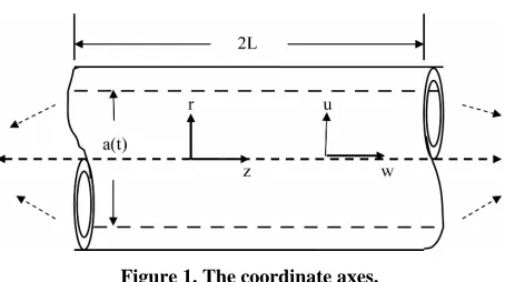
[image:1.595.321.539.563.708.2]In this paper, we investigate the problem of unsteady flow in contracting or expanding pipe, studied by Skalak and Wang [6] using long series methods. This problem Figure 1 for some particular choice of a(t), admits simi-larity transformation leading to a nonlinear differential
equation. The initial approximations enable us, in pro-posing a series expansion with polynomial coefficients to calculate enough terms (universal coefficients) by com-puter. Using a Domb-Sykes plot we find the nature and location of singularity restricting the convergence of the singularity. Then the problem is also analysed using Pade’ approximants and other useful techniques.
2. Mathematical Formulation
Let the inside tube be prescribed by a(t). The Navier- Stokes equations then admit similarity solutions if
0 1a t a t (2.1) where a0 and are constants.
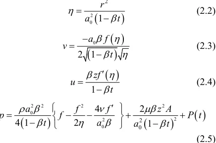
Let u and v be the velocities in cylindrical polar co- ordinate system in the directions of z and r respectively. Then the following transformations
2 0
2
1 r
a t
(2.2)
0
2 1
a f
v
t
(2.3)
1 zf u
t
(2.4)
2 2 2 2
0
2 2
0
2 0
4 2
4 1 2 1
a f f z A
p f
t a a t
P t
(2.5) where is normalized radius, p is the pressure, density, Kinematic viscosity. The constant A and the
Figure 1. The coordinate axes.
function are to be determined from the boundary conditions.
P t
The boundary conditions are on
, d ,d a
r a t v u
t
0, (2.6)
d
0, 0, 0
d u
r v
t
(2.7)
Using above equations, the Navier-Stokes equations take the form
2 2
f f S f f f f ff
0 (2.8) with the boundary conditions
0 00; or 0 0
0 1 0 1 1 f Lt f n
Lt n f
f f (2.9)
Here S is a squeeze number defined by
2 0 4 a S .
3. Method of Solution
We seek the solution of (2.8) in power series of S in the form
0
1
n n
n
f f S f
0
(3.1)
Substituting (3.1) into (2.8) and equating the like
powers of S on both sides, we get
0 2 0
f f
(3.2) and
1
1 1 1 1
0
2 2 n
n n n n n r r n r r
r
f f f f f f f f
(3.3)The relevant boundary conditions take the forms
0 0 0
0
0 0, 0, 1 0, 1 1
0 0, 0, 1 0, 1 0
n n
n
n
f Lt n f f f
f Lt n f f f
0
n
(3.4)
The solutions of the above equations up to O S
2 are2
2 3 4
2 3 4 5
0 1 2
2
5 7 2 1
9 6 3 18
1057 271 47 8 7 1
2700 270 54 27 180 1350
f f f 6 (3.5)
4. Computer Extended Series
As the series (3.5) is slowly converging it is not reliable to analyze the problem accurately with just few terms. It is essential to get higher approximations. As one pro-ceeds to higher approximations the algebra becomes cumbersome and it is difficult to calculate the terms manually. We propose a systematic series with polyno-mial coefficients which is quite useful and efficient in the calculation of higher approximations. In this method we get analytic structure of the solution just by generating universal coefficients. The series (3.5) gives solution for only up to S = 0.9. The forms of polynomial solutions (3.5) and nature of boundary conditions (3.4) suggest form of fn
to be of the form
,
2
2
1
1 k
n n k
n k
f A
(4.1)on substituting (4.1) into (3.3) and equating the coeffi-cients of various powers of on both sides we get re-currence relation An k, in the form
2 2 2 2 2 ,, 2 , 1
4
2 1 ,
2
1
2 2 2
2 2 2 3
, 1, 2 7 2
1 2 2 3
2
1
2 1
, 2
n N J n N J n N J
i n N i J i
n L
L k m N k J r r L r k L J r
A A A
A P N i J
N J N J N J
A A P k N k J r
n (4.2)
1 1 2 4
P k k k k k k1
2 2 1 1 8 1 2 1 2 4
P k k k k k k k k k k
3 2 1 4 2 1 4 1 4 1 4 1 1
P k k k k k k k k k k k k
4 2 2 1 2 2 1 2 2
P k k k k k k k
5 , 1 1 1 1 1 2 1 1
P k k k k k kk k 1
6 , 1 2 1 1 1 2 1 1 1 1 2 1 1 1 1 1 2 1 1 1 1
P k k k k k k k k k k k k k k 2
7 1 1 1 1 1 1 1 1 1 1 1
1 1 1 1 1 1
, 2 1 4 1 1 1 1 2
4 1 1 2 1 2
P k k k k k k k k k k k k k
k k k k k k
1 k
8 , 1 2 1 1 2 1 1 2 2 1 1 1 2 1 2 1 1 1 2 1 1 1 1
P k k k k k k k k k k k k k k 1
9 , 1 2 2 1 2 1 1 1 2 1 1
P k k k k k k k k1
and 1,1 5, 1,2 1
9 1
A A
8 The expression for f
1
2 ,
1 1
1 2 n n 1 2 1 2 1
n k n k
f S A k k k k k
k1
(4.3)
The expression for f
1
2
,
1 1
1 n n 1 2 2 1 1 2
n k n k
f S A k k k k k k k k k
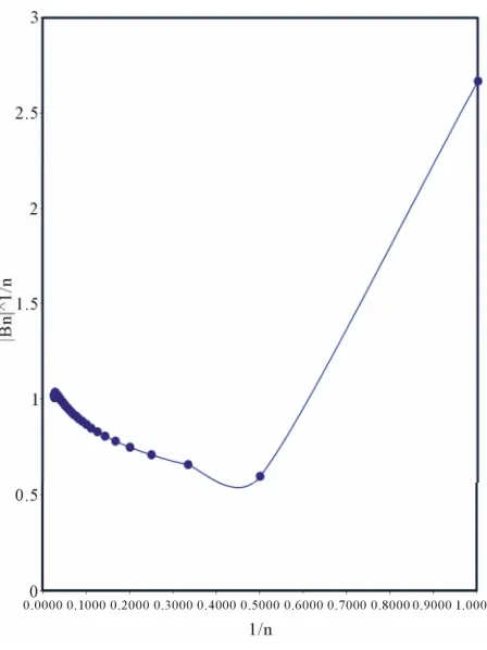
(4.4)The relation (4.3) and (4.4) represents the shear stress and pressure gradient respectively. Domb-Sykes plot (Figures 2 and 3), after extrapolation Vandyke [7], con-firms the radius of convergence of the series (4.3) and (4.4) to be = 0.98 & 0.97 respectively. The region of validity of the above series increased by considering Pade’ sum which are given in Tables 1 and 2.
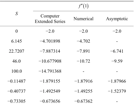
Table 1. Comparison of results for obtained by various methods for different S.
1 f
1
f
S Computer
Extended Series Numerical Asymptotic
0 −2.0 −2.0 −2.0
6.145 −4.701898 −4.702 -
22.7207 −7.887314 −7.891 −6.741
46.0 −10.677908 −10.72 −9.59
100.0 −14.791368 - -
−0.11487 −1.879155 −1.87916 −1.87966
−0.40737 −1.492549 −1.49255 −1.52379
[image:3.595.59.286.554.734.2]−0.73305 −0.673656 −0.67362 -
Figure 3. Domb-sykes plot for the coefficients of 4.4.
Table 2. Comparison of results for f
1 obtained by va- rious methods for different S. 1
f
S Computer
Extended Series Numerical Asymptotic
0.0 0.0 0.0 0.0
6.145 −13.808172 −13.808 -
22.7207 −48.556607 −48.658 −48.810
46.0 −96.517978 −96.55 −96.80
100.0 −206.110078 - -
−0.11487 0.311493 0.31149 0.311
−0.40737 1.175966 1.17596 1.14532
−0.73305 2.527063 2.52706 -
5. Conclusion
A new type of series is presented for studying the prob-lem of unsteady flow produced by squeezing of viscous fluid from a tube. Using recurrence relation (4.2) we
generate universal coefficients (An,k, k1, 2,3, , 2 n;
1, 2,3, , 25
n ). These coefficients in turn give univer-sal polynomial functions fn(η) . The
se-ries (4.3) gives
2, , 25
1,
n
1f and (4.4) represents f
1 have random sign pattern. Using Domb-Sykes plot (Figures 2 and 3), we locate the position ad identifying the nature of the nearest singularity of the series restricting the con-vergence. The series (4.3) and (4.4) are summed using Pade’ approximants Bender and Orszag [8]. Earlier series solution results were only for small value of S. But we are able to go upto S = 100 using Pade’ approximants. The results are in very close agreement with the numeri-cal findings Skalak and Wang [6].6. Acknowledgements
The research is supported by Manipal Academy of Higher Education, Manipal. (Under R & D scheme of M. I. T., Manipal) and one of us (KBC) wishes to thank the higher authority of Department of Collegiate Education, Govt. of Karnataka for their encouragement and support.
REFERENCES
[1] M. Y. Jaffrin and A. H. Shapiro, “Peristatic Pumping,” Annual Review of Fluid Mechanics, Vol. 3, 1971, pp. 13- 36. doi:10.1146/annurev.fl.03.010171.000305
[2] C. D. Bertram, C. J. Reymond and T. J. Pedley, “Map- ping of Instabilities during Flow through Collapsed Tubes of Differing Length,” Journal of Fluids and Structures, Vol. 4, No. 2, 1990, pp. 125-154.
doi:10.1016/0889-9746(90)90058-D
[3] T. W. Secomb, “Flow in a Channel with Pulsating Wall,” Journal of Fluid Mechanics, Vol. 88, No. 2, 1978, pp. 273-287. doi:10.1017/S0022112078002104
[4] M. Van Dyke, “Mathematical Approach in Hydrodynam- ics,” SIAM, Philadelphia, 1997.
[5] N. M. Bujurke and N. P. Pai, “Computer Extended Series Solution for Flow between Squeezing Plates,” Fluid Dy- namics Research, Vol. 16, No. 2-3, 1995, pp. 167-183.
doi:10.1016/0169-5983(94)00058-8
[6] F. M. Skalak and C. Y. Wang, “On the Unsteady Squeez- ing of a Viscous Fluid from a Tube,” Journal of the Aus- tralian Mathematical Society, Vol. 21, 1979, pp. 65-74. [7] M. Van Dyke, “Analysis and Improvement of Perturba-
tion Series,” Mathematics & Physical Sciences, Vol. 27, No. 4, 1974, pp. 423-456. doi:10.1093/qjmam/27.4.423 [8] C. M. Bender and S. A. Orszag, “Advanced Mathematical
[image:4.595.59.286.435.613.2]Appendix
Pade’ Approximants
The basic idea of Pade’ summation is to replace a power series
n n C R
by a sequence of rational functions of the form
00
N n n
N n
M M
n n n
A R
P R
B R
where we choose 0 without loss of generality. We determine the remaining (M + N + 1) coefficients 0 1
1
B
, ,
A A
2, , N; , ,0 1 2, , M
A A B B B B so that the first (M + N + 1) terms in the Taylor’s series expansion of match with first (M + N + 1) terms of power series
N M
P R
n n C R
.The resulting rational function is called a Pade’ approximant. If is a power series representa-tion of the funcrepresenta-tion
N M
P R
n n C R
f R
N M
P R f R , pointwise as , then in favourable cases . There are many methods for the construction of Pade’ approxi-mants. One of the efficient methods for constructing Pade’ approximants is recasting the series into continued fraction form. A continued fraction is an infinite se-quence of fractions whose (N + 1)th member has the form
,
N M
01
2
1
1 1 1 1
N
N N
D F R
D R D R
D R
D R
(A)
The coefficients Dn are determined by expanding the
terminated continued fraction F RN
in a Taylor seriesand comparing with those of the power series to be summed. An efficient procedure for calculating the coef-ficients Dn’s of the continued fraction (A) may be
de-rived from the algebraic identities (8.4.2a)-(8.4.2c) (Ben- der and Orszag [7]). Contrary to representations by power series, continued fraction representation may con- verge in regions that contain isolated singularities of the function to be represented, and in many cases conver-gence is accelerated. Based on these Dn’s we get
termi-nated continued fractions of various orders from the al-gorithms (8.4.7), (8.4.8a) and (8.4.8b) (Bender and Or-szag [7]).