Munich Personal RePEc Archive
On bootstrap validity for specification
tests with weak instruments
Doko Tchatoka, Firmin
University of Tasmania, School of Economics and Finance
31 March 2013
Online at
https://mpra.ub.uni-muenchen.de/47543/
On bootstrap validity for specification tests with
weak instruments
Firmin Doko Tchatoka
∗University of Tasmania
June 11, 2013
∗School of Economics and Finance, University of Tasmania, Private Bag 85, Hobart TAS 7001,
ABSTRACT
This paper investigates the asymptotic validity of the bootstrap for Durbin-Wu-Hausman (DWH) specification tests when instrumental variables (IVs) may be arbi-trary weak. It is shown that under strong identification, the bootstrap offers a better approximation than the usual asymptotic χ2 distributions. However, the bootstrap
provides only a first-order approximation when instruments are weak. This indicates clearly that unlike the Wald-statistic based on a k-class type estimator (Moreira et al., 2009), the bootstrap is valid even for the Wald-type of DWH statistics in the presence of weak instruments.
1.
Introduction
Specification tests of the type proposed by Durbin (1954), Wu (1973, 1974), and Hausman (1978), henceforth DWH tests, are widely used in applied work to decide whether the ordinary least squares (OLS) or instrumental variables (IV) method is appropriate. Although research on exogeneity testing in linear IV regressions is widespread1, most studies in this topic usually consider the case of strong instruments.
Recent studies focusing on the behavior of the DWH-type tests document that they never over-rejects the null hypothesis of exogeneity when IVs are weak. However, some of these tests can be overly conservative even in large-sample, and have low power when identification is weak.2 Doko Tchatoka and Dufour (2011b) propose a
size correction of these tests through the exact Monte carlo test procedure [ Dufour (2006)], which remains valid even when identification is weak and the sample size is small. However, the Monte Carlo test procedure suggested requires the a priori knowledge of the distribution of model disturbance, at least up to an unknown scale factor. But in practice, researchers usually do not know the exact distribution of the errors and implementing the simulated method can be difficult, even infeasible.
This paper aims to relax this distributional assumption by resorting to bootstrap methods. We mainly focus on linear structural models and establish the asymptotic validity of the bootstrap for DWH exogeneity tests, when IVs may be arbitrary weak (weak instruments).
Moreira et al. (2009) show in the context of hypotheses specified on structural
1
See, for example, Durbin (1954), Wu (1973, 1974, 1983a, 1983b), Revankar and Hartley (1973), Farebrother (1976), Hausman (1978), Revankar (1978), Dufour (1979, 1987), Hwang (1980), Kariya and Hodoshima (1980), Hausman and Taylor (1981), Spencer and Berk (1981), Nakamura and Nakamura (1981), Engle (1982), Holly (1982), Reynolds (1982), Smith (1983, 1984), Thurman (1986), Smith and Pesaran (1990), Ruud (1984, 2000), Newey (1985a, 1985b), Wong (1996), Ahn (1997), Baum, Schaffer and Stillman (2003).
2
See, for examples, Staiger and Stock (1997), Guggenberger (2010), and Doko Tchatoka and Dufour (2011a, 2011b). Staiger and Stock (1997, Section D) show that with weak IVs, the size of Hausman (1978) tests that exploit the residuals from the 2SLS estimation, and that of the Wu (1973)
T3test depends on identification strength through the concentration matrix. Since the concentration
parameters, that the bootstrap is valid for the score test. This not however the case for Wald-type tests based on the 2SLS or LIML estimators when IVs are weak. We use theLM and Wald interpretation of the DWH staistics in Engle (1982) and Smith (1983) to propose a slight modification of Moreira et al.’s (2009) bootstrap. Our anal-ysis of the bootstrap validity provides some new insights and extensions of Moreira et al.’s (2009). We show that when identification is strong, the bootstrap offers a better approximation than the usual asymptotic χ2 distributions (similar to Moreira
et al., 2009). However, the bootstrap provides only a first-order approximation when identification is weak, meaning that the bootstrap is valid even for the wald-type of the DWH test, despite the lack of identifiability. This contrasts with the bootstrap of the Wald-statistic based on the 2SLS or LIML estimators, which is invalid with weak IVs (Moreira et al., 2009).
The paper is organized as follows. Section 2 formulates the model and assump-tions, and presents the statistics studied. Section 3 presents the statistics and provides their Lagrange multiplier or Wald interpretation, following Engle (1982) and Smith (1983). Section 4 details the proposed bootstrap implemented as well as its validity in both strong and weak instrument setups. Conclusions are drawn in Section 5 and the proofs and auxiliary lemmas are presented in the Appendix.
2.
Framework
We consider the standard linear structural model described by the following equations:
y1 = y2β+Z1γ+u, (2.1)
y2 = Zπ2+Z1π1+v2 (2.2)
wherey1 andy2are n×1 vectors of observations on two endogenous variables, Z1 is a
n×k1 matrix of included exogenous variables,Z1 is an×k2 matrix instruments,u=
a vector of reduced form disturbances, β, γ ∈R are unknown structural parameters, while π1 ∈ Rk1 and π2 ∈ Rk2 is the unknown reduced-form coefficient vector. The
results in this paper can easily be extended to setups wherey2 contains more than one
regressors. We assume that Z = [Z1 : Z2] : n×k has full column-rank k=k1+k2.
The reduced-forms for y1 and y2 can be expressed from (2.1)-(2.2) as:
y1 = Z1(π1β+γ) +Z2π2β+v1
y2 = Z1π1+Z2π2+v2, (2.3)
where v1 = u+v2β. For any random matrix X, let Xi denote the i-th row of X,
written as column vector. Let Y = [y1 : y2] and define
Qn = vech
(Yn′, Zn′)′(Yn′, Zn′)= (f1(Yn′, Zn′), f1(Yn′, Zn′), . . . , fl(Yn′, Zn′)), (2.4)
where fi, i= 1, . . . , l, l = (k+ 2)(k+ 3)/2, k =k1+k2, are elements of the matrix
(Y′
n, Zn′)
′
(Y′
n, Zn′). Let ¯Qn =n−1Pni=1Qi denote the empirical mean of the Qi. The
following assumptions are made on the behavior of model variables.
Assumption 2.1 (a) Qn in (2.4) satisfies: E[kQnks] < ∞ for some s ≥ 3,
lim supktk→∞|E[exp(it′Qn)]|<1; and (b) when the sample size n converges to
infin-ity, the following convergence results hold jointly:
M1. n−1[u : v2]′[u : v2]
p →Σ =
σ2
u δ
δ σ2
v2
, n
−1Z′Z →p Q
Z, n−1Z′[u : v2]
p →0
M2. n−1/2Z′[u : v2]
d →
ψZu : ψZv2
, where ψZu = (ψ′Z1u, ψ
′
Z2u)
′ :k×1,
ψZv2 = (ψ′Z1v2, ψ′Z2V−2)′ :k×1, and vech
ψZu : ψZv2
∼N(0, Σ⊗QZ).
The first moment condition in Assumption 2.1-(a) holds ifE[k(Y′
n, Zn′)k2s]<∞, and
(1978)]. In Assumption 2.1-(b), M1 is the weak law of large numbers (WLLN) property, where IVs and disturbances are asymptotically uncorrelated, while M2 is the central limit theorem (CLT) property.
From Assumption 2.1, the exogeneity hypothesis of y2 can be expressed as:
H0 : δ= 0. (2.5)
We are concerned with the asymptotic validity of the bootstrap for the DWH statistics often used to assess H0,especially when identification is weak. Section 3 presents the
DWH statistics and their LM or Wald interpretation.
3.
Lagrange Multiplier and Wald Nature of the
Standard DWH Tests
We consider the statistics Tl, l = 2, 3,4, by Wu (1973, 1974) and three alternative
Hausman (1978) type statistics, namely,Hj, j = 1, 2, 3. LetA1 =In−Z1(Z1′Z1)−1Z1′
and A2 =In−Z(Z′Z)−1Z′ denote the orthogonal matrices to the spaces spanned by
the columns of Z1 and Z, respectively. The statistics Tl and Hj can be expressed in
the unified formulation as:
Tl = κl(˜β−βˆ)2/ω˜2l , l = 2, 3, 4, (3.1) Hj = n(˜β−βˆ)2/ωˆ2j, j = 1,2, 3 (3.2)
where ˆβ = (y′
2A1y2)−1y2′A1y1 and ˜β = [y′2(A1−A2)y2]−1y2′(A1 −A2)y1 are the OLS
and IV estimators of β,respectively, and
˜
ˆ
ω21 = ˜σ2ωˆ−iv1−σˆ2ωˆ−ls1, ωˆ
2
2 = ˜σ2∆,ˆ ωˆ23 = ˆσ2∆,ˆ
ˆ
∆ = ˆω−iv1−ωˆls−1, ωˆiv =y2′(A1−A2)y2/n, ωˆls=y′2A1y2/n,
˜
σ2 = (y1−y2β˜)′A1(y1−y2β˜)/n, σˆ2 = (y1−y2βˆ)′A1(y1−y2βˆ)/n,
˜
σ22 = ˆσ2−(˜β−βˆ)2/∆, κˆ 2 =n−2−k1, κ3 =κ4 =n−1−k1.
Engle (1982) and Smith (1983) show that each statistic in (3.1)-(3.2) has a score or Wald interpretation. The statisticsT2,T4,andH3 areLM-type, whileT3,H1,andH2
are quasi-Wald type.3 Under H
0 and if further Assumption 2.1-(b) holds, all DWH
statistics have the usual chi-square asymptotic distributions if model identification is strong. However, T3, H1, and H2 are overly conservative, and all DWH tests
have a low power if IVs are weak, even in large-sample. We question whether a bootstrap technique can improve4 the properties of the DWH tests, with or without
weak instruments.
4.
Bootstrap Validity for DWH Tests
Let ˆπ = (Z′Z)−1Z′y
2 denotes the OLS estimator of π = (π′1, π′2)′ in the first stage
regression (2.2). Let ˆθ be an estimator ofβand ˆγ those ofγ.The bootstrap procedure consists of the following steps:
3
See Smith (1983) for the score interpretation (Eqs. [6] and [9]) and for the quasi-Wald inter-pretation (Eqs. [7], [8] and [10]). The regression interinter-pretation of these statistics is provided in Hausman (1978), Dufour (1979, 1987), Wooldridge (2009), and Doko Tchatoka and Dufour (2011b).
4
Due to theLM nature ofT2,T4,H3,and the result in Moreira et al. (2009), one can project the
bootstrap validity for these statistics. But formal proof needs to be established, especially because the primary focus in Moreira et al. (2009) is not exogeneity testing, and there is no discussion in Moreira et al. (2009) related to exogeneity testing. On the other hand, because of the Wald nature of
T1,T3,H1,H2,and the bootstrap invalidity result for the Wald-statistic in Moreira et al. (2009), it
1. From observed data, compute ˆπ and ˆθ along with all other things necessary to get the realizations of the statistics Tl, Hj, and the residuals from the reduced-form equation (2.3): ˆv1 = y1 −Z1(ˆπ1ˆθ+ ˆγ)−Z2πˆ2ˆθ, vˆ2 = y2−Zπ.ˆ These residuals are
then re-centered by subtracting sample means to yield (˜v1, v˜2).
2. For each bootstrap sample r = 1, . . . , B, data are generated as:
y∗1 = Z1∗(ˆπ1ˆθ+ ˆγ) +Z2∗πˆ2βˆ+v1∗, y∗2 =Z∗πˆ+v2∗ (4.1)
where Z∗ = [Z∗
1 : Z2∗] and (v1∗, v2∗) are drawn independently from the empirical
distribution of Z and (˜v1, v˜2). The corresponding bootstrap statistics T∗ r
l and H∗
r
j
are then computed for each bootstrap sample r = 1, . . . , B.
3. The simulated bootstrap p-value is obtained as the proportion of bootstrap statistics that are more extreme than the statistics computed from observed data.
4. The bootstrap test rejects the null hypothesis of exogeneity at level α if its p-value is less than α.
The above bootstrap steps, though similar to those by Moreira et al. (2009), have a slight difference in the appropriate5 estimator of ˆθ to be used; see fn.4 for further
details. We now show the asymptotic validity of the bootstrap.
5
Moreira et al. (2009) show that ˆθmust be strongly consistent, i.e.,
ˆ π p
→ π and ˆθˆπ p
→θπ, (4.2)
4.1.
High-order approximation with strong instruments
In this section, we focus on the case whereπ 6= 0 is fixed (strong IVs). We can express the bootstrap DHW statistics Tl∗ and H∗j based on the re-centering residuals as:
Tl∗ =
√
nG( ¯˜Q∗n)2, H∗j =√nG˜( ¯˜Q∗n)2 for all l and j (4.3)
where ¯˜Qnand ¯˜Q∗nare analogous of ¯Qnin (2.4). ¯˜Qnis based on the sample re-centering
residuals and ¯˜Q∗
n is based on the bootstrap sample residuals. The functionsG(.) and
˜
G(.) are real-valued Borel measurable functions on Rl, which satisfy G( ¯˜Qn) = 0 and
˜
G( ¯˜Qn) = 0, due to the re-centered mechanism [similar to Eqs. (A.5)-(A.6) in the
Appendix]. Under strong identification, all derivatives of order s and less of the functions G(.) and ˜G(.) are continuous. So, Edgeworth-type expansion6 applies and
we have the following theorem.
Theorem 4.1 Bootstrap validity with Strong IVs. Suppose Assumption
2.1 is satisfied. Under H0 and if further π 6= 0 is fixed, we have:
kP∗(Tl∗ ≤x)−[Φ(x) +
s−2
X
m=1
n−m/2pmT
l(x;Fn,
ˆ
β,ˆπ)Φ(x)]2 k∞ = o(n(s−2)),
kP∗(H∗j ≤x)−[Φ(x) +
s−2
X
m=1
n−m/2pm
Hj(x;Fn,β,ˆ ˆπ)Φ(x)] 2 k
∞ = o(n
(s−2)
) as n→ ∞
for all l and j, where pm
Tl and p
m
Hj are polynomials in x with coefficients depending on
ˆ
β, π,ˆ and the moments of the distribution Fn of Q˜
∗
n = vech
( ˜Y∗′
n , Z˜∗
′
n)
′
( ˜Y∗′
n , Z˜∗
′
n)
conditional on Fˆn={(Y′
1, Z1′), . . . , (Yn′, Zn′)}; Φ(.) is the cdf of N(0.1) and k.k∞ is
the supremum norm.
First, Theorem 4.1 shows that the bootstrap approximates the empirical Edge-worth expansion in Lemma A.1 up to the o(n(s−2)) order. This is not surprising because the conditional moments of Q∗
n, given the data ˆFn, converge almost surely
6
to those of Qn when identification is strong. Second, the results shows that the
error based on the bootstrap simulation is of order n−1. Therefore, the bootstrap
offers a better approximation than the usual asymptotic χ2 distributions, even for
the Wald-type versions of the DWH statistics.
4.2.
First-order Validity with Weak Instruments
High-order approximation of the limiting distributions of the bootstrap as in Theorem
4.1is not achievable now due to the lack of identification. Indeed, whenπ2 =π0/√n
where π0 is a k2 ×1 constant vector, the functions G(.) and ˜G(.) in (4.3) are
non-differentiable.7 So, the Edgeworth expansion is not applicable. However, we can
prove the following theorem on the first-order approximation of the bootstrap when IVs are weak.
Theorem 4.2 Bootstrap validity with weak IVs. Suppose Assumptions
2.1 and H0 are satisfied. If for some δ >0, E(kZik4+δ, kvik2+δ)<∞, then we have:
Tl∗ |Fˆn d
→ χ2(1), Hj∗ |Fˆn→d χ2(1) a.s., for all l= 2, 3,4; j = 1,2, 3
whenπ=π0/√n, π0 is ak×1constant vector, andFˆn ={(Y1′, Z1′), . . . , (Yn′, Zn′)}.
First, since the statistics T2, T4,and H3 are LM-type and following Moreira et al.
(2009), the bootstrap validity for these statistics is predictable. However, the result of the Wald-type of the DWH statistics, T3, H1, and H2, is less obvious, because the
bootstrap is not valid for the Wald-statistic of Hβ : β =β0 (see Moreira et al., 2009).
The key reason behind the bootstrap validity for the Wald-statistic here is that their asymptotic distributions, even when δ 6= 0, do not depend on the unknown nuisance parameter8 β, with or without weak IVs. Meanwhile, the asymptotic distribution of
7
Note that all DWH statistics depends ony′
2(A1−A2)y2/n.However, it is straightforward to see
that the derivative of the functionsG(.) and ˜G(.) with respect toy′
2(A1−A2)y2/nis not well-defined
whenπ= 0 or does not exist ifπ=π0cn for any sequencecn↓0.So,G(.) and ˜G(.) are not smooth
when IVs are weak, and Edgeworth-type expansion does not apply.
8
the Wald-statistic of Hβ : β = β0, based on 2SLS or LIML, depends heavily9 on β
under the weak instrument scenario.
4.3.
Monte Carlo experiment
We use simulation to examine the size performance of the proposed bootstrap. The DGP is described10 by Eqs. (2.1) and (2.2) where the n rows of [u, v
2] are drawn
i.i.d. with mean zero and unit variance, and the correlation between ui and v2i is
set at ρ = 0 under H0. Z2 contains k2 instruments, each generated i.i.d N(0,1)
independently of [u, v2]. We vary k2 in {2, 5, 20} within the experiment, but the
results are consistent with alternative values. The true value of β is set at 2 and the reduced-form coefficient π2 is chosen as π2 = ( µ
2
nkZ2π0k) 1/2
π0, where π0 is a vector of
ones,µ2 is the concentration parameter characterizing the strength of the IVs. In this
experiment, µ2 varies in{0, 413,1000}.11To account for non-normal errors, [u, v 2] is
generated following Kotz et al. (2000):
ui = a+bε1i+cε21i+dε31i, v2i =a+bε2i+cε22i+dε32i (4.4)
where (ε1i, ε2i)′ i.i.d.
∼ N(0, I2) for all i = 1, . . . , n. We consider two setups: (1) a =
c = d = 0 and b = 1 (normal errors), and a = c = 0, b = d = 1/√22 (non-normal errors) such that12 Sknew= 0 andKurt≈27.72.
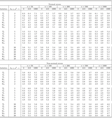
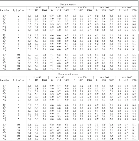
Table 1 presents the results for the standard DWH tests, and Table 2 reports those of the bootstrap tests. The first column of each table contains the test statistics, the second reports the number of IVsk2, while the others present, for each sample size (n)
9
See Nelson and Startz (1990); Staiger and Stock (1997); Dufour (1997, 2003); Wang and Zivot (1998), among others.
10
There is no exogenousZ1 in the simulations but the results do not alter when such exogenous
IVs are included.
11
Following Hansen et al. (2008), µ2
= 0 is a design of complete non-identification,µ2
= 413 designs weak identification, andµ2
= 1000 is for strong identification.
12
and the IV strength (µ2), the empirical rejections of the tests. The bootstrap rejection probability is estimated using 10,000 pseudo-sample sets, each of size n varying in
{50,100, 200, 500, 1000}. The nominal level for both the standard and bootstrap tests is 5%. It is clear from Table 1 that the standard Wald-type of the DWH tests, namely, T3, H1, and H2, are highly conservative with weak IVs (see columns µ2 = 0
and µ2 = 413). The rejection frequencies of the LM-type tests —T
2, T4, and H3—
are close to the nominal level of 5% even when IVs are weak. These results are similar for normal and non-normal errors. Meanwhile, Table 2 shows clearly that the bootstrap method improves the size of the tests, especially for the Wald-type of the DWH tests. As seen, even the rejection frequencies of T3, H1, and H2 are very close
to the nominal level, no matter how weak the IVs are, with or without normal errors, even with relatively small-sample sizes.
5.
Conclusion
This paper considers the standard linear IV models and investigates the asymptotic validity of the bootstrap for the standard DWH exogeneity tests. We propose a slight modification of Moreira et al.’s (2009) bootstrap, which provides some new insights and extensions of earlier results. When identification is strong, we show that the bootstrap offers a better approximation of the distributions of the statistics than the usual asymptotic χ2 distributions. However, it provides only a first-order
Acknowledgments
Table 1. Rejection frequencies (in %) of the standard DWH tests Normal errors
n= 50 n= 100 n= 200 n= 500 n= 1000
Statistics k2↓ µ2→ 0 413 1000 0 413 1000 0 413 1000 0 413 1000 0 413 1000
T2 2 6.3 6.4 7.1 5.7 5.2 5.7 6.0 5.6 5.7 6.2 5.6 5.6 6.1 5.5 5.6
T2 2 5.6 5.4 5.0 5.1 5.1 5.4 4.9 5.2 5.0 4.9 5.2 5.0 4.9 4.7 4.9
T3 2 0.1 4.0 4.2 0.0 3.7 4.6 0.0 3.7 4.2 0.1 2.9 3.8 0.0 2.0 3.6
T4 2 4.7 4.7 4.3 4.8 4.7 4.9 4.7 5.0 4.8 4.9 5.1 4.9 4.9 4.7 4.9
H1 2 0.1 3.5 3.6 0.0 3.4 4.2 0.0 3.6 4.0 0.1 2.8 3.7 0.0 1.9 3.6
H2 2 0.1 4.2 4.3 0.0 3.8 4.7 0.0 3.8 4.3 0.1 2.9 3.8 0.0 2.0 3.6
H3 2 5.0 4.9 4.5 4.9 4.8 5.1 4.8 5.1 4.9 4.9 5.1 4.9 4.9 4.7 4.9
T2 5 5.5 5.5 5.4 5.3 5.4 5.4 4.9 5.5 5.1 4.7 5.2 5.0 5.3 4.9 5.2
T3 5 0.3 4.5 4.7 0.3 4.9 5.0 0.3 4.6 4.8 0.4 4.2 4.6 0.3 3.9 4.5
T4 5 5.0 4.8 4.8 4.9 5.2 5.1 4.8 5.3 5.0 4.6 5.1 5.0 5.3 4.9 5.1
H1 5 0.2 3.9 4.0 0.3 4.5 4.6 0.2 4.5 4.6 0.3 4.2 4.6 0.2 3.8 4.5
H2 5 0.3 4.8 4.9 0.3 4.9 5.1 0.3 4.7 4.8 0.4 4.2 4.7 0.3 3.9 4.5
H3 5 5.2 5.1 5.0 5.1 5.2 5.2 4.8 5.4 5.0 4.6 5.2 5.0 5.3 4.9 5.1
T2 20 5.6 5.1 5.7 5.0 5.3 5.4 5.0 5.2 5.1 4.9 4.5 5.1 5.2 4.9 5.2
T3 20 3.3 4.5 5.1 3.0 4.9 5.0 2.8 5.0 4.8 2.9 4.3 4.9 2.8 4.6 5.1
T4 20 4.8 4.5 5.1 4.7 4.9 5.0 4.9 5.1 4.9 4.8 4.5 5.0 5.2 4.9 5.2
H1 20 2.7 3.9 4.4 2.7 4.6 4.6 2.7 4.8 4.6 2.8 4.2 4.9 2.8 4.5 5.1
H2 20 3.5 4.6 5.3 3.1 5.0 5.1 2.8 5.0 4.9 2.9 4.3 5.0 2.9 4.6 5.1
H3 20 5.0 4.7 5.3 4.8 5.1 5.2 4.9 5.2 5.0 4.9 4.5 5.0 5.2 4.9 5.2
Non-normal errors
n= 50 n= 100 n= 200 n= 500 n= 1000
Statistics k2↓ µ2→ 0 413 1000 0 413 1000 0 413 1000 0 413 1000 0 413 1000
T2 2 5.0 6.3 6.1 5.2 5.0 5.6 4.8 5.0 5.0 5.0 5.0 4.7 4.9 4.9 5.4
T3 2 0.0 5.0 5.4 0.0 3.8 5.0 0.0 3.4 4.3 0.1 2.8 3.8 0.0 2.2 4.0
T4 2 4.2 5.6 5.6 4.8 4.7 5.4 4.6 4.9 4.8 5.0 5.0 4.6 4.9 4.9 5.4
H1 2 0.0 4.4 4.8 0.0 3.5 4.7 0.0 3.3 4.1 0.0 2.8 3.7 0.0 2.1 3.9
H2 2 0.0 5.2 5.6 0.0 3.9 5.0 0.0 3.5 4.4 0.1 2.8 3.8 0.0 2.2 4.0
H3 2 4.5 5.9 5.7 5.0 4.9 5.5 4.7 5.0 4.9 5.0 5.0 4.6 4.9 4.9 5.4
T2 5 5.3 6.0 5.9 5.2 5.4 5.9 5.2 5.1 5.0 5.0 4.3 5.2 4.9 4.8 5.0
T3 5 0.3 5.3 5.2 0.3 4.8 5.6 0.3 4.3 4.5 0.2 3.6 4.7 0.2 3.7 4.5
T4 5 4.6 5.5 5.3 4.8 5.2 5.7 5.0 4.8 4.9 4.9 4.3 5.2 4.9 4.8 5.0
H1 5 0.2 4.7 4.6 0.2 4.5 5.2 0.2 4.2 4.3 0.2 3.5 4.6 0.2 3.7 4.5
H2 5 0.3 5.5 5.4 0.3 4.9 5.6 0.3 4.4 4.6 0.2 3.6 4.7 0.2 3.7 4.5
H3 5 4.8 5.6 5.4 4.9 5.2 5.8 5.1 4.9 4.9 4.9 4.3 5.2 4.9 4.8 5.0
T2 20 5.5 5.8 5.8 5.1 5.2 5.6 5.2 5.1 5.4 4.9 5.2 5.0 4.8 4.9 4.8
T3 20 3.5 5.2 5.1 2.8 4.8 5.1 3.1 4.8 5.1 2.7 4.8 4.8 2.6 4.6 4.7
T4 20 4.9 5.2 5.2 4.8 4.9 5.2 5.0 4.9 5.1 4.8 5.1 4.9 4.8 4.9 4.8
H1 20 2.8 4.6 4.5 2.6 4.5 5.0 2.9 4.6 5.0 2.7 4.8 4.8 2.6 4.6 4.7
H2 20 3.8 5.4 5.3 2.9 4.9 5.3 3.1 4.8 5.2 2.8 4.9 4.9 2.6 4.7 4.7
H3 20 5.1 5.5 5.3 4.9 5.0 5.3 5.1 5.0 5.2 4.9 5.1 5.0 4.8 4.9 4.8
Table 2. Rejection frequencies (in %) of the bootstrap DWH tests Normal errors
n= 50 n= 100 n= 200 n= 500 n= 1000
Statistics k2↓ µ2→ 0 413 1000 0 413 1000 0 413 1000 0 413 1000 0 413 1000
T∗
2 2 6.3 6.4 7.1 5.7 5.2 5.7 6.0 5.6 5.7 6.2 5.6 5.6 6.1 5.5 5.6
T∗
3 2 6.5 6.4 7.1 5.9 5.2 5.7 6.1 5.6 5.7 6.3 5.6 5.6 6.2 5.5 5.6
T∗
4 2 6.3 6.4 7.1 5.7 5.2 5.7 6.0 5.6 5.7 6.2 5.6 5.6 6.1 5.5 5.6
H∗
1 2 6.5 6.4 7.1 5.9 5.2 5.7 6.1 5.6 5.7 6.3 5.6 5.6 6.2 5.5 5.6
H∗
2 2 6.5 6.4 7.1 5.9 5.2 5.7 6.1 5.6 5.7 6.3 5.6 5.6 6.2 5.5 5.6
H∗
3 2 6.3 6.4 7.1 5.7 5.2 5.7 6.0 5.6 5.7 6.2 5.6 5.6 6.1 5.5 5.6
T∗
2 5 6.8 5.9 5.9 6.6 6.0 6.7 7.2 5.6 5.4 6.2 5.8 5.6 7.6 5.8 5.1
T∗
3 5 6.8 5.9 5.9 6.6 6.0 6.7 7.2 5.6 5.4 6.2 5.8 5.6 7.6 5.8 5.1
T∗
4 5 6.8 5.9 5.9 6.6 6.0 6.7 7.2 5.6 5.4 6.2 5.8 5.6 7.6 5.8 5.1
H∗
1 5 6.8 5.9 5.9 6.6 6.0 6.7 7.2 5.6 5.4 6.2 5.8 5.6 7.6 5.8 5.1
H∗
2 5 6.8 5.9 5.9 6.6 6.0 6.7 7.2 5.6 5.4 6.2 5.8 5.6 7.6 5.8 5.1
H∗
3 5 6.8 5.9 5.9 6.6 6.0 6.7 7.2 5.6 5.4 6.2 5.8 5.6 7.6 5.8 5.1
T∗
2 20 6.0 5.9 6.1 7.1 6.3 6.7 6.6 6.3 6.3 6.7 5.2 5.1 7.1 5.8 5.5
T∗
3 20 6.0 5.9 6.1 7.1 6.3 6.7 6.6 6.3 6.3 6.7 5.2 5.1 7.1 5.8 5.5
T∗
4 20 6.0 5.9 6.1 7.1 6.3 6.7 6.6 6.3 6.3 6.7 5.2 5.1 7.1 5.8 5.5
H∗
1 20 6.0 5.9 6.1 7.1 6.3 6.7 6.6 6.3 6.3 6.7 5.2 5.1 7.1 5.8 5.5
H∗
2 20 6.0 5.9 6.1 7.1 6.3 6.7 6.6 6.3 6.3 6.7 5.2 5.1 7.1 5.8 5.5
H∗
3 20 6.0 5.9 6.1 7.1 6.3 6.7 6.6 6.3 6.3 6.7 5.2 5.1 7.1 5.8 5.5
Non-normal errors
n= 50 n= 100 n= 200 n= 500 n= 1000
Statistics k2↓ µ2→ 0 413 1000 0 413 1000 0 413 1000 0 413 1000 0 413 1000
T∗
2 2 6.4 5.8 6.4 6.0 5.7 6.0 5.7 5.2 5.2 5.5 5.3 5.8 5.5 5.0 5.2
T∗
3 2 6.4 5.8 6.4 5.9 5.7 6.0 5.9 5.2 5.2 5.7 5.3 5.8 5.7 5.0 5.2
T∗
4 2 6.4 5.8 6.4 6.0 5.7 6.0 5.7 5.2 5.2 5.5 5.3 5.8 5.5 5.0 5.2
H∗
1 2 6.4 5.8 6.4 5.9 5.7 6.0 5.9 5.2 5.2 5.7 5.3 5.8 5.7 5.0 5.2
H∗
2 2 6.4 5.8 6.4 5.9 5.7 6.0 5.9 5.2 5.2 5.7 5.3 5.8 5.7 5.0 5.2
H∗
3 2 6.4 5.8 6.4 6.0 5.7 6.0 5.7 5.2 5.2 5.5 5.3 5.8 5.5 5.0 5.2
T∗
2 5 6.9 6.6 5.9 6.0 5.3 6.0 6.3 5.3 5.5 6.7 5.8 5.1 6.9 5.5 5.4
T∗
3 5 6.9 6.6 5.9 6.0 5.3 6.0 6.3 5.3 5.5 6.7 5.8 5.1 6.9 5.5 5.4
T∗
4 5 6.9 6.6 5.9 6.0 5.3 6.0 6.3 5.3 5.5 6.7 5.8 5.1 6.9 5.5 5.4
H∗
1 5 6.9 6.6 5.9 6.0 5.3 6.0 6.3 5.3 5.5 6.7 5.8 5.1 6.9 5.5 5.4
H∗
2 5 6.9 6.6 5.9 6.0 5.3 6.0 6.3 5.3 5.5 6.7 5.8 5.1 6.9 5.5 5.4
H∗
3 5 6.9 6.6 5.9 6.0 5.3 6.0 6.3 5.3 5.5 6.7 5.8 5.1 6.9 5.5 5.4
T∗
2 20 6.1 6.2 6.2 6.2 6.2 6.5 6.4 5.9 6.2 7.1 5.9 5.8 6.9 5.7 5.1
T∗
3 20 6.1 6.2 6.2 6.2 6.2 6.5 6.4 5.9 6.2 7.1 5.9 5.8 6.9 5.7 5.1
T∗
4 20 6.1 6.2 6.2 6.2 6.2 6.5 6.4 5.9 6.2 7.1 5.9 5.8 6.9 5.7 5.1
H∗
1 20 6.1 6.2 6.2 6.2 6.2 6.5 6.4 5.9 6.2 7.1 5.9 5.8 6.9 5.7 5.1
H∗
2 20 6.1 6.2 6.2 6.2 6.2 6.5 6.4 5.9 6.2 7.1 5.9 5.8 6.9 5.7 5.1
H∗
3 20 6.1 6.2 6.2 6.2 6.2 6.5 6.4 5.9 6.2 7.1 5.9 5.8 6.9 5.7 5.1
APPENDIX
A.
Auxiliary Lemmata and Proofs
This appendix presents some useful auxiliary lemmas and their proofs, as well as the proofs of the main theorems in the text.
A.1.
Auxiliary Lemmata
Lemma A.1 Suppose Assumption 2.1is satisfied and that π6= 0 is fixed. Under H0, we have:
(a) kP(√n(˜β−βˆ)
˜
ωl ≤
x)−[Φ(x) + s−2
X
m=1
n−m/2pmT
l(x; ˜F , π)Φ(x)]k∞=o(n
(s−2)/2
) (A.1)
kP(√n(˜β−βˆ)
ˆ
ωj ≤
x)−[Φ(x) + s−2
X
m=1
n−m/2pmHj(x; ˜F , π)Φ(x)]k∞=o(n
(s−2)/2
) (A.2)
(b) kP(Tl≤x)−[Φ(x) + s−2
X
m=1
n−m/2pmT
l(x;F,
π)Φ(x)]2k∞=o(n
(s−2)
) , (A.3)
kP(Hj≤x)−[Φ(x) + s−2
X
m=1
n−m/2pmHj(x; ˜F , b0,π)Φ(x)]
2
k∞=o(n
(s−2)
) (A.4)
for all l and j, where pm
Tl and p
m
Hj are polynomials in x with coefficients depending on
moments of the distribution F of Qn and π, and Φ(.) is the cdf of a standard normal
random variable.
Lemma A.2 Suppose Assumption 2.1 is satisfied. If for some δ > 0, we have E(kZik2+δ, kvik2+δ) < ∞, then E
∗
(|Z∗
jiv∗mi|2+δ) is bounded a.s. under H0, for all
j = 1, . . . , k and m = 1, 2; where Z∗ and v∗ = [v∗
1 : v2∗] are the bootstrap draws
from the empirical distribution of Z and the re-centered residuals ˜v = [˜v1 : ˜v2].
Corollary A.3 Under the assumptions of LemmaA.2, E∗(|Z∗
jiu∗i|2+δ)is boundeda.s.
under H0 for all j = 1, . . . , k and m= 1, 2; where u∗ =v∗
Lemma A.4 Suppose Assumption 2.1 is satisfied. If for some δ > 0, E(kZik4+δ, kvik2+δ)<∞, then under H0, we have:
Z∗ u∗
/√n Z∗ v∗ 2/ √ n √
n(W∗
′
1
n −
W′1
n )
|Fˆn →d N
0,
diag(σ2
u, σv2)⊗QZ 0
0 Σw
a.s.
where W = (w1, . . . , wn), wi = vech(ZiZi′), W∗ = (w∗1, . . . , w∗n), w∗i =
vech(Z∗
iZ∗
′
i )∈R
k(k+1)/2
, Σw =var(wi), and 1 is a (n by 1) constant vector of ones,
ˆ
Fn ={(Y′
1, Z1′), . . . , (Yn′, Zn′)}.
Lemma A.5 Suppose Assumption 2.1 is satisfied. If for some δ > 0, E(kZik4+δ, kvik2+δ)<∞, then under H0, we have:
√
n(˜β∗−βˆ∗) ˜
ω∗l |Fˆn
d
→ N(0, 1),
√
n(˜β∗−βˆ∗) ˆ
ω∗j |Fˆn
d
→N(0,1) a.s.
when π = π0/√n, π0 is a (k by 1) constant vector (and π0 = 0 is allowed), where
˜
β∗, βˆ∗, ω˜l∗, ωˆ∗j are the bootstrap counterparts ofβ,˜ β,ˆ ω˜l, andωˆj defined in(3.1)-(3.2).
A.2.
Proofs
To shorten the exposition, note that the proofs of Theorem 4.1 and Lemma A.2 are similar to those in Moreira et al. (2009) and are omitted.
Proof of Lemma A.1 First, it is easy to see that Tl = cn
l
√
n(˜βω˜−βˆ)
l
2
and
Hj =
√
n(˜βωˆ−βˆ)
j
2
for alll and j,wherecnl = 1 +o(1). Now, we can observe
√
n(˜βω˜−ˆβ)
l
and √n(˜βωˆ−βˆ)
j as:
√
n(˜β−βˆ)
˜
ωl = √n(y
′
2y2/n)−1(y′2y1/n)−[(y′2Z/n)(Z′Z/n)−1(Z′y2/n)]−1[(y′2Z/n)(Z′Z/n)−1(Z′y1/n)
q
y′
1My2y1
n [(
y′
2PZy2
n )
−1−(y′2y2
n )
−1]−[(y′2y2
n )
−1(y′2y1
n )−( y′
2PZy2
n )
−1(y′2PZy1
n )]2 = √n(y
′
2y2/n)−1(y′2u/n)−[(y′2Z/n)(Z′Z/n)−1(Z′y2/n)]−1[(y′2Z/n)(Z′Z/n)−1(Z′u/n)
q
y′
1My2y1
n [(
y′
2PZy2
n )
−1−(y2′y2
n )
−1]−[(y′2y2
n )
−1(y′2y1
n )−( y′
2PZy2
n )
−1(y′2PZy1
n )]2
√
n(˜β−βˆ)
ˆ
ωj = √n(y
′
2y2/n)−1(y′2y1/n)−[(y′2Z/n)(Z′Z/n)−1(Z′y2/n)]−1[(y′2Z/n)(Z′Z/n)−1(Z′y1/n)
q
y′
1My2y1
n [(
y′
2PZy2
n )
−1−(y′2y2
n )
−1]
= √n(y
′
2y2/n)−1(y′2u/n)−[(y′2Z/n)(Z′Z/n)−1(Z′y2/n)]−1[(y′2Z/n)(Z′Z/n)−1(Z′u/n)
q
y′
1My2y1
n [(
y′
2PZy2
n )
−1−(y′2y2
n )
−1]
= √nG˜( ¯Qn)under H= 0√n[ ˜G( ¯Qn)−G˜(µ)] (A.6)
where G(.) and ˜G(.) are real-valued Borel measurable functions in Rl such that
G(µ) = G(E(Qn)) = 0 and ˜G(µ) = ˜G(E[Qn]) = 0 under H0.13 Since π 6= 0 is
fixed (strong identification), all derivatives of G(.) and ˜G(.) of order s and less are continuous in the neighborhood of µ = 0. So, if further Assumption 2.1-(b) holds, then (A.1)-(A.2) follow directly from Bhattacharya and Ghosh (1978, Theorem 2) and (A.3)-(A.4) hold by the definition ofTl and Hj.
Proof of Lemma A.4 Let (c′, d′)′ be a nonzero vector with c = (c′
1, c′2)′ ∈ R2k
and d∈Rk(k+1)/2. Define
Xni = c′1Zi∗u∗i/ √
n+c′2Zi∗v2∗i/√n+d′(w∗i −w¯)/√n
where [u∗
i : v∗2i] is the i-th bootstrap draw of the (re-centered) residuals, and ¯w =
n−1Pn
i=1wi, wi =vech(ZiZi′)∈R
k(k+1)/2
, and w∗
i =vech(Zi∗Z∗
′
i )∈R
k(k+1)/2 .
We want to use the Cram´er-Wold device. For this, it suffices to show Xni satisfies
all the conditions of the Liapunov Central Limit Theorem.
1. The first condition is obvious. Indeed, we haveE∗(Xni) = 0 by the independence
between Z∗ and [u∗
i :v2∗i],and the fact that E
∗
{[u∗
i :v2∗i]}= 0.
2. The second condition is E∗(X2
ni)<∞. Again, by the independence between Z∗
13
This holds becauseE(y′
and [u∗i :v2∗i] and because u∗ is uncorrelated with v2∗ under H0, we have
E∗(Xni2) = n−1
c′1
Z′u˜u˜′Z
n
c1+c′2
Z′v˜ 2˜v2′Z
n
c2+d′Σ˜wd
<∞ a.s.,
where ˜Σw =n
−1Pn
i=1(wi−w¯)(wi−w¯)′.
3. To check the final condition of the Liapunov Central Limit Theorem, it requires to show that limn→∞Pni=2E
∗
(|Xni|2+δ) = 0 a.s. for some δ > 0. Now, note
that
n
X
i=2
E∗[|Xni|2+δ] = n−δ/2n−1 n
X
i=2
E∗h|c′1Zi∗u∗i +c′2Zi∗v2∗i+d′(w∗i −w¯)|2+δi
≤ C1n−δ/2E ∗h
|c′1Zi∗u∗i|2+δ+|c′2Zi∗v2∗i|2+δ+|d′(w∗i −w¯)|2+δi
≤ C2n−δ/2
k X j=1
|c1j|2+δE
∗
[|Zji∗u∗i|2+δ] +
k
X
j=1
|c2j|2+δE
∗
[|Zji∗v2∗i|2+δ]+
+ C2n−δ/2
k(k+1)/2
X
p=1
|dp|2+δE
∗
[|w∗pi−
1 n n X j=1 wji
|2+δ]
= C2n−δ/2[A1+A2+A3]
for large enough constants C1 and C2. From Lemma A.2 and Corollary A.3,
we have A1 =O(1) and A2 =O(1) a.s. If further E[kZik4+δ]<∞, then e have
A3 = O(1) a.s. Therefore, we get limn→∞Pni=2E ∗
[|Xni|2+δ] = 0 a.s., and the
last condition of the Liapunov Central Limit Theorem is satisfied. Lemma A.4
is the Central Limit Theorem property once we realize thatplimn→∞ Z
′u˜u˜′Z
n
=
σ2
uQZ, plimn→∞
Z′v˜
2˜v′2Z
n
=σ2
v2QZ, and plimn→∞( ˜Σw) =Σw.
Proof of Lemma A.5 First, note that E∗(Z∗′Z∗/n) = Z′Z/n, E∗(Z∗′u∗/n) =
Z′u/n,˜ E∗
(Z∗′
v∗
2/n) =Z′˜v2/n, and E ∗
[(u∗ :v∗
the Markov law of large numbers entails that
Z∗′
Z∗
n − Z′Z
n |Fˆn
a.s. → 0, Z∗
′
u∗
n − Z′u˜
n |Fˆn
a.s. → 0, Z∗
′
v∗ 2
n − Z′v˜
2
n | Fˆn
a.s. → 0 1
n(u
∗ :v∗
2)′(u∗:v∗2)−
1
n(˜e: ˜v2)
′(˜u: ˜v
2)|Fˆn a.s.
→ 0; a.s.
Since Z′Z/n →p Q
Z, and Z′v˜2/n
p
→ 0, we have Z′u/n˜ →p 0 and if H
0 holds, (˜u :
˜
v2)′(˜u : ˜v2)/n
p
→ diag(σ2
u, σ2v2). So, it is clear that: Z
∗′
Z∗/n a.s.→ Q
Z, Z∗
′
u∗/n a.s.→ 0,
Z∗′
v∗ 2/n
a.s.
→ 0, and (u∗ :v∗
2)′(u∗ :v2∗)/n
a.s.
→ diag(σ2
u, σ2v2) under H0.
Now, from the above results along with Lemma A.4 and the fact that
π = c/√n, we have: y∗′
2 y∗2/n = π′0(Z∗ ′
Z∗/n2)π
0 + 2π′
0Z∗ ′
v∗
2/n3/2 + v∗ ′
2 v∗2/n |
ˆ
Fn a.s.→ σ2
v2 and y
∗′ 2 PZ∗y∗
2 = (y∗ ′
2 Z∗/
√
n)(Z∗′
Z∗/n)−1(Z∗′
y∗ 2/
√
n) | Fˆn →d (ψ
Zv2 + QZπ0)′Q−1
Z (ψZv2 + QZπ0) a.s., where ψZv2 ∼ N(0, σ
2
v2QZ). Therefore, we have
˜
β∗−βˆ∗ = (y2∗′PZ∗y∗ 2)−1(y∗
′
2 PZ∗u∗)−(y∗ ′
2 y∗2/n)−1(y∗ ′
2 u∗/n) = (y∗ ′ 2 PZ∗y∗
2)−1(y∗ ′
2 PZ∗u∗) +
op(1)|Fˆn d
→[(ψZv2+QZπ0)′Q−1
Z (ψZv2+QZπ0)]
−1(ψ
Zv2+QZπ0)
′Q−1
Z ψZu a.s. under
H0. Similarly, we can show that ˜ω∗
2
l /n, ωˆ∗
2
j /n |Fˆn→a.s σu2[(π0ψZv2 +QZ)
′Q−1
Z (ψZv2+ QZπ0)]−1 a.s. for all l and j. Thus we get
√
n(˜β∗−βˆ) ˜
ω∗l |Fˆn
d → σ1
u
[(ψZv2+QZπ0)
′Q−1
Z (ψZv2 +QZπ0)]
−1/2(ψ
Zv2 +QZπ0)
′Q−1
Z ψZu √n(˜β∗
−βˆ∗) ˆ
ω∗j |Fˆn
d → σ1
u
[(ψZv2+QZπ0)
′Q−1
Z (ψZv2 +QZπ0)]
−1/2(ψ
Zv2 +QZπ0)
′Q−1
Z ψZu a.s.
Moreover,ψZuandψZv2 are independent and jointly normal under H0(see also Lemma
A.4), thus we have σ1u[(ψZv2+QZπ0)′Q−1
Z (ψZv2+QZπ0)]
−1/2(ψ
Zv2+QZπ0)
′Q−1
Z ψZu |
ψZv2 ∼N(0, 1).Because the conditional distribution of
1
σu[(ψZv2+QZπ0)′Q
−1
Z (ψZv2+ QZπ0)]−1/2(ψ
Zv2 +QZπ0)′Q
−1
Z ψZu, given ψZv2, does not depend on ψZv2, it is equal
to the unconditional distribution. It follows that √n(˜β
∗
−βˆ) ˜
ω∗
l |
ˆ
Fn →d N(0, 1) and
√n(˜β∗
−βˆ∗) ˆ
ω∗
j |
ˆ
Proof of Theorem 4.2 First, recall that T∗
l =
√
n(˜β∗−βˆ∗) ˜
ω∗
l
2
and H∗j =
√
n(˜β∗−βˆ∗) ˆ
ω∗
j
2
. By Lemma A.5, we have √n(˜β
∗
−βˆ∗) ˜
ω∗
l |
ˆ
Fn →d N(0, 1) and √n(˜β
∗
−βˆ∗) ˆ
ω∗
j |
ˆ
Fn →d N(0, 1) a.s. It is clear that T∗
l | Fˆn d
→ [N(0, 1)]2 ≡ χ2(1) and H∗
j | Fˆn d →
[N(0, 1)]2 ≡χ2(1) a.s.
References
Ahn, S. , 1997. Orthogonality tests in linear models. Oxford Bulletin of Economics and Statistics 59, 83–186.
Baum, C., Schaffer, M. , Stillman, S. , 2003. Instrumental variables and GMM: Esti-mation and testing. Technical report, Department of Economics, Boston College, MA, Boston, USA MA.
Bhattacharya, R. N. , Ghosh, J. , 1978. On the validity of the formal edgeworth expansion. The Annals of Statistics 6, 434–451.
Doko Tchatoka, F. , Dufour, J.-M. , 2011a. Exogeneity tests and estimation in IV regressions. Technical report, Department of Economics, McGill University, Canada Montr´eal, Canada.
Doko Tchatoka, F., Dufour, J.-M., 2011b. On the finite-sample theory of exogeneity tests with possibly non-gaussian errors and weak identification. Technical report, Department of Economics, McGill University, Canada Montr´eal, Canada. Dufour, J.-M., 1979. Methods for Specification Errors Analysis with Macroeconomic
Applications PhD thesis University of Chicago. 257 + XIV pages. Thesis com-mittee: Arnold Zellner (Chairman), Robert E. Lucas and Nicholas Kiefer. Dufour, J.-M. , 1987. Linear Wald methods for inference on covariances and weak
Advances in the Statistical Sciences: Festschrift in Honour of Professor V.M. Joshi’s 70th Birthday. Volume III, Time Series and Econometric Modelling . D. Reidel, Dordrecht, The Netherlands, pp. 317–338.
Dufour, J.-M., 1997. Some impossibility theorems in econometrics, with applications to structural and dynamic models. Econometrica 65, 1365–1389.
Dufour, J.-M. , 2003. Identification, weak instruments and statistical inference in econometrics. Canadian Journal of Economics 36(4), 767–808.
Dufour, J.-M., 2006. Monte carlo tests with nuisance parameters: A general approach to finite-sample inference and nonstandard asymptotics in econometrics. Journal of Econometrics 138, 2649–2661.
Durbin, J., 1954. Errors in variables. Review of the International Statistical Institute 22, 23–32.
Engle, R. F. , 1982. A general approach to Lagrange multiplier diagnostics. Journal of Econometrics 20, 83–104.
Farebrother, R. W., 1976. A remark on the Wu test. Econometrica 44, 475–477. Guggenberger, P., 2010. The impact of a Hausman pretest on the size of the hypothesis
tests. Econometric Theory 156, 337–343.
Hansen, C., Hausman, J. , Newey, W. , 2008. Estimation with many instrumental variables. Journal of Business and Economic Statistics 26(4), 398–422.
Hausman, J., 1978. Specification tests in econometrics. Econometrica 46, 1251–1272. Hausman, J., Taylor, W. E., 1981. A generalized specification test. Economics Letters
8, 239–245.
Hwang, H.-S. , 1980. Test of independence between a subset of stochastic regressors and disturbances. International Economic Review 21, 749–760.
Kariya, T. , Hodoshima, H. , 1980. Finite-sample properties of the tests for inde-pendence in structural systems and LRT. The Quarterly Journal of Economics 31, 45–56.
Kotz, S., Balakrishnan, N., Johnson, N., 2000. Continuous Multivariate Distributions second edn. John Wiley & Sons, New York.
Li, J. , 2006. The block bootstrap test of hausman’s exogeneity in the presence of serial correlation. Economics Letters 91, 76–82.
Moreira, Marcelo J.and Porter, J., Suarez, G., 2009. Bootstrap validity for the score test when instruments may be weak. Journal of Econometrics 149, 52–64. Nakamura, A., Nakamura, M., 1981. On the relationships among several specification
error tests presented by Durbin, Wu and Hausman. Econometrica 49, 1583–1588. Nelson, C., Startz, R., 1990. The distribution of the instrumental variable estimator and its t-ratio when the instrument is a poor one. The Journal of Business 63, 125–140.
Newey, W. K., 1985a. Generalized method of moments specification testing. Journal of Econometrics 29, 229–256.
Newey, W. K., 1985b. Maximum likelihood specification testing and conditional mo-ment tests. Econometrica 53(5), 1047–1070.
Revankar, N. S. , 1978. Asymptotic relative efficiency analysis of certain tests in structural sysytems. International Economic Review 19, 165–179.
Reynolds, R. A. , 1982. Posterior odds for the hypothesis of independence be-tween stochastic regressors and disturbances. International Economic Review 23(2), 479–490.
Ruud, P., 2000. An Introduction to Classical Econometric Theory. Oxford University Press, Inc., New York.
Ruud, P. A. , 1984. Tests of specification in econometrics. Econometric Reviews 3(2), 211–242.
Smith, R. J., 1983. On the classical nature of the wu-hausman statistics for indepen-dence of stochastic regressors and disturbance. Economics Letters 11, 357–364. Smith, R. J. , 1984. A note on likelihood ratio tests for the independence between a
subset of stochastic regressors and disturbances. International Economic Review 25, 263–269.
Smith, R. J. , Pesaran, M. , 1990. A uni ¨Oed approach to estimation and orthogonal-ity tests in linear single-equation econometric models. Journal of Econometrics 44, 41–66.
Spencer, D. E. , Berk, K. N. , 1981. A limited-information specification test. Econo-metrica 49, 1079–1085.
Staiger, D. , Stock, J. H. , 1997. Instrumental variables regression with weak instru-ments. Econometrica 65(3), 557–586.
Thurman, W., 1986. Endogeneity testing in a supply and demand framework. Review of Economics and Statistics 68(4), 638–646.
Wang, J., Zivot, E., 1998. Inference on structural parameters in instrumental variables regression with weak instruments. Econometrica 66(6), 1389–1404.
Wooldridge, J. M. , 2009. Introductory Econometrics: A Modern Approach fourth edn. South-Western, USA.
Wu, D.-M., 1973. Alternative tests of independence between stochastic regressors and disturbances. Econometrica 41, 733–750.
Wu, D.-M., 1974. Alternative tests of independence between stochastic regressors and disturbances: Finite sample results. Econometrica 42, 529–546.
Wu, D.-M. , 1983a. A remark on a generalized specification test. Economics Letters 11, 365–370.