http://www.scirp.org/journal/ijcns ISSN Online: 1913-3723 ISSN Print: 1913-3715
New Blind Recognition Method of SCLD and
OFDM in Alpha-Stable Noise
Junlin Zhang, Bin Wang, Yang Wang
National Digital Switching System Engineering and Technological R&D Centre, Zhengzhou, China
Abstract
This paper deals with modulation classification under the alpha-stable noise condition. Our goal is to discriminate orthogonal frequency division multip-lexing (OFDM) modulation type from single carrier linear digital (SCLD) modulations in this scenario. Based on the new results concerning the genera-lized cyclostationarity of these signals in alpha-stable noise which are pre-sented in this paper, we construct new modulation classification features without any priori information of carrier frequency and timing offset of the received signals, and use support vector machine (SVM) as classifier to dis-criminate OFDM from SCLD. Simulation results show that the recognition accuracy of the proposed algorithm can be up to 95% when the mix signal to noise ratio (MSNR) is up to −1 dB.
Keywords
Modulation Recognition, Generalized Second-Order Cyclic Statistics, OFDM, Alpha-Stable Noise
1. Introduction
With wide application of OFDM, the recognition of OFDM signal has become a hot issue in various fields of applications among cognitive radio and military ap-plications. Algorithms for the recognition of OFDM versus SCLD signals in AWGN scenario have been reported in [1]-[6]. The algorithm proposed in [1] is based on the signal empirical distribution function to recognize OFDM. Fourth- and sixth-order signal moments are employed in [2] to identify OFDM and sin-gle-carrier. Wavelet analysis is also employed to distinguish OFDM and SCLD in [3] [4]. The algorithm proposed is based on the second-order cyclic cumulate to recognize OFDM versus SCLD signals under time dispersive channel in [5]. Based on the spectrum analysis, an algorithm was proposed to recognize OFDM in [6]. The above results were developed under the simplified assumption of ad-How to cite this paper: Zhang, J.L., Wang,
B. and Wang, Y. (2017) New Blind Recog-nition Method of SCLD and OFDM in Alpha-Stable Noise. Int. J. Communica-tions, Network and System Sciences, 10, 240-251.
https://doi.org/10.4236/ijcns.2017.105B024 Received: April 20, 2017
ditive white Gaussian noise channel. But, many noise processes are impulsive in nature. Impulsive channels have been arisen in underwater (ice-cracks), atmos-pheric (thunderstorms) environments, and other mobile communication prob-lems [7]. Impulsive noise can be modelled as alpha-stable distribution process which is different from Gaussian noise. When the communication channel in nature is impulsive channel modelled as alpha-stable distribution process, the existing recognition algorithms of OFDM versus SCLD would become invalid, because the impulsive noise does not have second-order and higher order statis-tics. For this reason, we study the recognition of OFDM against SCLD signals in alpha-stable noise here. In this paper, we extract new modulation classification features from the new results concerning the generalized cyclostationarity of OFDM and SCLD signals in alpha-stable noise, and use support vector machine (SVM) as classifier to these signals. The recognition algorithm avoids the need for timing and carrier recovery and the estimation of signal and noise powers. Simulation results show that the proposed method have good performances in alpha-stable noise.
The rest of the paper is organized as follows. The SCLD and OFDM signal models is presented in Sections 2, the proposed recognition algorithm is intro-duced in Section 3 and simulation results are discussed in Section 4. Finally, our conclusions are presented in Section 5.
2. Signal Models
The received signal can be written as, ( ) ( ) ( )
r t =s t +w t (1)
where s t( ) means the transmitted signal, w t( ) is alpha-stable noise.
If the modulation type of the transmitted signal is OFDM, s t( ) can be represented by s t( )OFDM, which is expressed as,
1
2 2 ( )
, 0
( )
( )
c k s s
K
j f t j k f t lT T j
OFDM k l
k l
s s
s t Ae e a e
g t lT T
π π µ
θ
µ
− ∞
∆ ∆ − −
= −∞
=
× − −
∑ ∑
(2)where A is the amplitude, θ is the phase, ∆fc is the carrier frequency offset,
0≤µ≤1 is the timing offset, g t( ) is the overall impulse response of the transmit and receive filters, K is the number of subcarriers of the OFDM
sig-nal, ak l, is the symbol transmitted on the kth subcarrier over the lth symbol pe-riod, ∆fk is the frequency separation between two adjacent subcarriers, Ts is the OFDM symbol period, and Ts=Tu+Tcp. The data symbols
{ }
ak l, areas-sumed to be zero-mean independent and identically distributed (i.i.d.) random variables, with values drawn either from a quadrature amplitude modulation (QAM) or phase shift keying (PSK) constellation.
If the modulation type of the transmitted signal is SCLD, s t( ) can be represented by s t( )SCLD, which is expressed as,
2
( ) j j f tc ( )
SCLD l c c
l
s t Be eθ π b g t lT µT
∞ ∆
=−∞
where B is the amplitude, θ is the carrier phase, ∆fc is the frequency offset,
c
T is the symbol period, 0≤µ≤1 is the timing offset, g t( ) is the overall impulse response of the transmit and receive filters, bl is the symbol transmit-ted in the lth symbol period. The data symbols
{ }
bl are assumed to be ze-ro-mean independent and i.i.d., with values drawn either from a quadrature am-plitude modulation (QAM) or phase shift keying (PSK) constellation.The alpha-stable noise w t( ) is defined by its characteristic function, since a closed form expression for its probability density function (pdf) is not always available. The characteristic function φ( )u is given by [8],
[
]
(
)
( )u exp jau uα 1 j sgn( ) ( , )u u
φ = −γ + β ω α (4)
In (4), ω α( , )u and sgn( )u is given as,
tan( / 2) 1
( , )
(2 / ) log 1
u
u
πα α
ω α
π α
≠
= =
(5)
and
1 0
sgn( ) 0 0
1 0
u
u u
u
>
= =
− <
(6)
where α, γ , and a are the characteristic exponent, dispersion, and location, respectively. Without loss of generality, noise employs standard symmetric al-pha-stable distribution-SαS as model. Because the SαS noise do not have finite second moment, its noise variance loses meaning. So a mixed signal to noise ra-tio-MSNR is employed, MSNR is given by [8],
2
10 lg( s )
MSNR= σ γ (7)
where 2
s
σ represents the signal variance and γ is dispersion of alpha-stable noise.
3. The Recognition Algorithm of OFDM and SCLD in
Alpha-Stable Distributed Noise
3.1. The Generalized Second-Order Cyclic Statistics of OFDM and SCLD
( )
1 ( ) ( )f r t r t
r t
=
(8)
where r t
( )
represents the received signal.The autocorrelation function of signal f r t
( )
can be expressed as,[ ] [
*]
* * ( , ) ( ) ( ) ( ) ( ) ( ) ( ) ( ) ( ) ( ) ( ) ( ) ( ) ( ) ( )G t E f r t f r t
s t s t E
s t w t s t w t
w t w t s t w t s t w t
τ τ τ τ τ τ τ τ = + + = + + + + + + + + + + (9)
When MSNR is higher enough, s t( ) w t( ) , (9) can be approximated as,
[ ] [
*]
* * ( , ) ( ) ( ) ( ) ( ) ( ) ( ) ( ) ( ) ( ) ( ) ( , ) ( , ) s wG t E f r t f r t
s t s t w t w t
E E
s t s t s t s t
G t G t
τ τ τ τ τ τ τ τ = + + + ≈ + + + = + (10)
where ( , ) ( ) (* )
( ) ( )
s
s t s t
G t E
s t s t
τ τ τ + = + , * ( ) ( ) ( , ) ( ) ( ) w
w t w t
G t E
s t s t
τ τ
τ
+ = +
, G ts( , )τ represents autocorrelation information
of s t( ). When s t( ) w t( ) , the amplitude of noise is suppressed. Obviously, when processing the received signal r t( ) with nonlinear transformation, the unique features of signal s t( ) are maintained in G ts( , )τ , and the amplitude of noise is effectively limited. For the OFDM signal, (2) can be put into (10) and (10) becomes * 1 2 2 0 1 2 0 1
2 ( )
* *
0 1
2 ( )
0 ( ) ( ) ( , ) ( ) ( ) ( ) ( ) ( ) ( ) ( ) ( ) ( ) ( ) ( ) c k k k k OFDM K
j f j k f t
k k K
j k f t k
k K
j k f t k
k
s s
K
l j k f t
k k
s t s t
G t E
s t s t
e a t e g t
E
a t e g t
a t e g t
t lT T
a t e g t
π τ π
π π τ π τ τ τ τ τ τ δ µ τ τ − − ∆ ∆ = − ∆ = − − ∆ + = − =−∞ ∆ + = + = ⋅ + = + + × ⊗ − − + +
∑
∑
∑
∑
[
]
1 12 2 * 2 ( )
0 0
1 1
2 2 ( )
0 0
*
( ) ( )
( ) ( )
( ) ( ) ( )
c k k
k k
K K
j f j k f t j k f t
k k
k k
K K
j k f t j k f t
k k
k k
s s
l
e a t e a t e
E
a t e a t e
P g t P g t t lT T
π τ π π τ
π π τ
τ
τ
τ δ µ
∞ − − − ∆ ∆ − ∆ + = = − − ∆ ∆ + = = ∞ =−∞ + = + × + ⊗ − −
∑
∑
∑
∑
∑
∑
(11)the data is assumed to be i.i.d.. Hence, (11) can be further re-written as,
[
]
)
* 1 2 2 , 0 * ( ) ( ) ( , ) ( ) ( ) ( ) ( ) ( ) ( ) c k OFDM Kj f j k f
k s k
s s
l
s t s t
G t E
s t s t
e C t e P g t
P g t t lT T
π τ π τ
τ τ
τ
τ δ µ
− − ∆ − ∆ = ∞ =−∞ + = + = × + ⊗ − −
∑
∑
(12)where ( ) ( ) ( ) 0
( ) ( )
k k
s
a t a t
C t E
s t s t
τ τ + = ≥ + , 1 2 0
( ) ( ) k
K
j k f t
k k
s t a t e π
−
∆
=
=
∑
,( )
⋅∗represents the complex conjugate, P
[ ]
⋅ standfor operator, which maintain the phase of signal, δ ⋅( ) is the Dirac delta func-tion and ⊗ is convolution. From (12) one can see that GOFDM( , )tτ is a peri-odic function with fundamental periperi-odic Ts. The autocorrelation function can be easily expressed as a Fourier series, and the Fourier transform of (12) yields
{
}
[
]
)
1 2 2 0 * 2 ( , ) ( , ) ( ) ( ) ( ) ( ) c k OFDM OFDM Kj f j k f
s k
j t
s s
l
G G t
e C t e P g t
P g t t lT T e dt
π τ π τ
π ε
ε τ τ
τ δ µ
− ∞ − ∆ − ∆ −∞ = ∞ − =−∞ = ℑ = × + ⊗ − −
∑
∫
∑
(13)where ℑ ⋅
{}
denotes the Fourier transform. Furthermore, by expressing theconvolution, using a change of variables and the identity 1
1
( s) ( s )
l l
t lT lT
T
δ δ ε
∞ ∞
−
−∞ =−∞
ℑ − = −
∑
∑
, one can show that (13) becomes[
]
[
]
1
2 2 *
0
2
1
2 2 2
0
* 2 1
2 ( , ) ( ) ( ) ( ) ( ) 1 ( ) ( ) ( ) ( ) 1 c k
c s k
c
OFDM
K
j f j k f
s k j t s l K
j f j T j k f s k s j t s l j f s G
e C t e P g t P g t
t lT T e dt
e e e C t P g t
T
P g t e dt lT
e T
π τ π τ
π ε
π τ πεµ π τ
π ε
π
ε τ
τ
δ µ
τ δ ε
− ∞ − ∆ − ∆ −∞ = ∞ − −∞ − +∞ − ∆ − − ∆ −∞ = +∞ − − =−∞ − ∆ = + ⊗ − − = × + − =
∑
∫
∑
∑
∫
∑
[
]
1 2 2 0* 2 1
( )
( ) ( )
0
s k
K
j T j k f s k
j t
s
e e C t
P g t P g t e dt lT
else
τ πεµ π τ
π ε τ ε − +∞ − − ∆ −∞ = − − × + =
∑
∫
(14)where 1 2 (1 )
0 sin( ) ( ) sin( ) k k K
j k f j K f k
k
k k
K f
e e
f
π τ π τ π τ
τ π τ − − ∆ − ∆ = ∆
Ξ = =
∆
∑
. Note that (14) give theanalytical expressions for the generalized second-order cyclic statistics at
1
s lT
ε = − and certain delay. According to (14), when
1 / fK Tu
yields significant peaks. Meanwhile, the magnitude peaks of GOFDM( , )ε τ are visible atτ =Tu and
1
s lT
ε = −
, with l as an integer.
As one can notice, when processing the received signal r t
( )
with nonlineartransformation, the modulated information of received signal r t
( )
ismain-tained in the GOFDM( , )tτ . For the OFDM signal, significant peaks occur in the vicinity of τ =Tu and
1
s lT
ε = − .
{
}
( , ) w G tτ
ℑ stands for noise interference, and its impact has been suppressed due to the nonlinear transformation.
Similarly, for the SCLD signal, we obtain
[
]
2 2
1
* 2 1
( , ) ( ) ( )
( ) ( )
c c
j f j T
SCLD c
j t
c l
G T e e b t P g t
P g t e dt lT
π τ πεµ
π ε
ε τ
τ δ ε
∞ − ∆ − − −∞ +∞ − − =−∞ = × + −
∫
∑
(15)where b t( ) is information data transmitted and the data is assumed to be i.i.d.. According to (15), the magnitude peaks of GSCLD( , )ε τ are visible at τ =0
and 1
c lT
ε = − .
3.2. The Generalized Cyclostationarity-Based Recognition Method of OFDM and SCLD Signals
Based on the above results on signal the generalized cyclic statistics, here we de-velop a novel algorithm for the recognition of OFDM and SCLD signals in al-pha-stable noise.
Under the assumption of no aliasing, for the discrete-time signal
1
( ) ( )
s
n tf
r n =r t = − , obtained by sampling the continuous-time signals r t
( )
at thesampling rate fs. According to the discussed in Section 3.1, we obtain
[
]
*[
]
* * ( , ) ( ) ( ) ( ) ( ) ( ) ( ) ( ) ( ) ( ) ( ) ( , ) ( , ) s wG n E f r n f r n
s n s n w n w n
E E
s n s n s n s n
G n G n
τ τ τ τ τ τ τ τ = ⋅ + + + ≈ + + + = + (16)
Then, for the OFDM signal, G ns( , )τ can be written as
[
]
)
1 1 1
2 2
0
*
( , ) ( )
( ) ( ) ( )
c s k s
K
j f f j k f f
OFDM s
k
s s
l
G n e C n e
P g n P g n n lN N
π τ π τ
τ
τ δ µ
− − − − ∆ − ∆ = ∞ =−∞ = × × + ⊗ − −
∑
∑
(17)where ( ) ( ) ( ) 0
( ) ( )
k k
s
a n a n
C n E
s n s n
τ τ + = ≥ + , 1 2 0
( ) ( ) k
K
j k f n
k k
s n a n e π
−
∆
=
=
∑
, Ns denotes OFDM symbol length, ands u cp
N =N +N , Nu = fs /∆fK is the useful symbol length and Ncp is the cyclic
{
}
[
]
)
[
]
1 1 1 1 1 2 2 0 * 2 0 12 2 2
0 * 2 ( , ) ( , ) ( ) ( ) ( ) ( ) 1 ( ) ( ) ( ) (
c s k s
s c s k s
OFDM OFDM
K
j f f j k f f
s n k j n s l K
j N j f f j k f f
s n k
s
j n
G G n
e C n e P g n
P g n n lN n e
e e e C n
N
P g n P g n e
π τ π τ
πυ
πυµ π τ π τ
πυ
υ τ τ
τ δ
τ δ υ
− − − − − − ∆ − ∆ = ∞ − =−∞ − − − ∆ − ∆ = − = ℑ = × + ⊗ − − = × +
∑
∑
∑
∑ ∑
1 ) s l lN +∞ − =−∞ −∑
(18)where 1 2 1 (1 ) 1 1
1 0
sin( )
( )
sin( )
k s k s
K
j k f f j K f f k s
k
k k s
K f f
e e
f f
π τ π τ π τ
τ π τ − − − − − ∆ − ∆ − = ∆
Ξ = =
∆
∑
, the significant peaks of Ξk( )τ can be obtained at τ = fs/∆ =fK Nu. Furthermore, from (18) it can be noticed that magnitude peaks are visible at τ = Nu and
1
/ s
l N
υ= − ,
with l as an integer.
Similarly, for the SCLD signal, we obtain
{
}
[
]
(
)
1 2 2 1* 2 1
( , ) ( , )
( ) ( )
( ) ( )
c s c
SCLD SCLD
j f f j N c
n
j n
c l
G G n
N e e b n P g n
P g n e lN
π τ πυµ
πυ
υ τ τ
τ δ υ
− − ∆ − − +∞ − − =−∞ = ℑ = × + −
∑
∑
(19)where ( ) ( ) ( ) 0
( ) ( )
b n b n
C n E
b n b n
τ τ + = + ≥
, b n( ) is information of data transmitted and the data is assumed to be independent and identically distributed. Nc de-notes symbol length of SCLD. According to (19), magnitude peaks of are visible at τ=0 and υ lNc1
−
= , with l as an integer.
When comparing (18) and (19), one can easily notice the additional factor ( )
k τ
Ξ which appears in the expression of the generalized cyclic statistics of the OFDM signal. One can easily show that significant peaks of the generalized cyc-lic statistics of OFDM signal yields at τ=0 and υ lNc1
−
= . The existence of such a peak in the magnitude of the generalized cyclic statistics of the OFDM signal (at τ = Nu and υ=0) is employed as discriminating feature to identify OFDM against SCLD signals.
The estimate of the generalized cyclic statistics Gˆ ( , )υ τ exist the estimation error factor which vanishes asymptotically is N→ ∞. Due to the existence of estimation error factor, the estimator seldom exactly zero in practice, even if υ
is not at generalized cycle frequencies. In order to decrease the impact of estima-tion error factor, referencing [10], the modulaestima-tion classificaestima-tion features are given as,
( )
1( )
†ˆ ˆ ˆ
r r r
WCυ − Cυ
Ψ = Σ (20)
where ˆ Re
{
ˆ( , )} {
Im ˆ( , )}
r
the covariance matrix
(
)
{
}
{
(
)
}
(
)
{
}
{
(
)
}
20 21 20 21
20 21 21 20
Re / 2 Im / 2
ˆ
Im / 2 Re / 2
r
Q Q Q Q
Q Q Q Q
+ −
Σ =
+ −
(21)
with covariance estimators are respectively given by,
(
)
( )
(
)
( )
( )
(
)
1 /2
1 * 1
2,1
1 /2
1
2 2
2 2
w w
w v
Q W v F vW
F vW
ω πυ π
πυ π
−
− −
=− − −
= +
× +
∑
(22)
and
(
)
( )
(
)
( )
( )
(
)
1 /2
1 1
2,0
1 /2
1
2 2
2 2
w w
w v
Q W v F vW
F vW
ω πυ π
πυ π
−
− −
=− − −
= −
× +
∑
(23)
where 1 * 2
0
( ) Ww ( ) ( ) j w
F υ =
∑
=− r w+τ r l e− πυ , ω( )
v is a spectral window of support w (odd).
According to the above analysis, the steps of recognizing OFDM against SCLD modulations may be obtained as follows:
Step 1: The magnitude of the generalized second-order cyclic statistics ˆ ( , )
Gυ τ of the received signal is estimated. Firstly, the discrete-time signal r n( ) obtained by sampling the continuous-time signal r t
( )
at the sampling rate fs.Then, the nonlinear transformation function in (8) is used to map received sig-nal r n( ). Finally, the normalization magnitude of the second-order cyclic sta-tistics Gˆ ( , )υ τ of the transformed signal f r t
( )
is estimated.Step 2: The modulation classification features Ψ is extracted from Gˆ ( , )υ τ . Search the maximum Gˆ (0, )τ value at υ=0 section, and the delays τ in the interval [ρKmin,ρKmax] (with and as the minimum and maximum number of
subcarriers that we consider). Then, the modulation classification features Ψ is extracted with (20).
Step 3: The modulation type is decided. Classify the test signal by employing the SVM classifier defined in the training procedure.
4. Simulation Results and Analysis
A. Simulation setup
The number of training and test sequences is respectively set to 100 for each class at each MSNR.
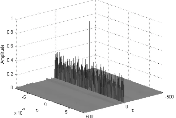
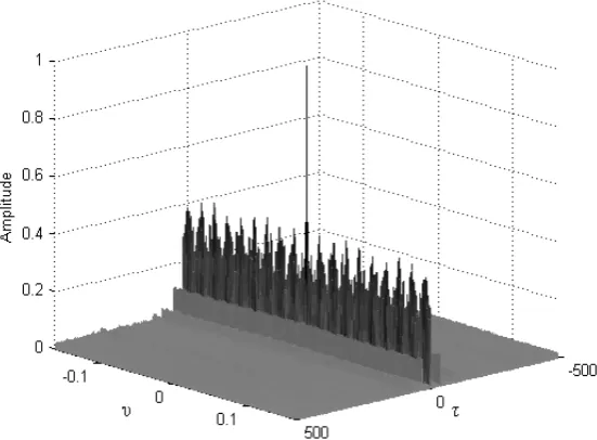
B. Generalized second-order cyclic statistics magnitude estimates for the OFDM and SCLD signals
The estimated magnitude of the generalized cyclic statistics of OFDM and SCLD is plotted. For SαS noise, MSNR = 10 dB and α =1.5.
When comparing results presented in Figure 1 and Figure 2, one can notice that the second-order cyclic spectrum of OFDM signal is destroyed by al-pha-stable noise, but the generalized second-order cyclic statistics of OFDM signal yields significant peaks at τ = Nu and
1
/ s
l N
[image:9.595.235.512.300.482.2]υ= − . Figure 3 shows that the generalized second-order cyclic statistics of SCLD signal can keep the cha-racteristics of second-order cyclic statistics. However, Figure 4 shows that the second-order cyclic statistics of SCLD signal is destroyed by alpha-stable noise. From Figure 1 and Figure 3 one can notice that the existence of such a peak in
Figure 1. Generalized second-order cyclic statistics of OFDM signal.
[image:9.595.233.518.524.715.2]Figure 3. Generalized second-order cyclic statistics of SCLD signal.
Figure 4. Second-order cyclic statistics of SCLD signal.
the magnitude of the generalized cyclic statistics of the OFDM signal (at τ = Nu
and 1
/ s l N
υ= − ) is employed as discriminating feature to recognize OFDM against SCLD signals.
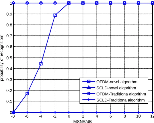
C. Performance of proposed recognition algorithm
Without loss of generality, set α=1.5. 200 tests for each MSNR value, and observation interval is set to 0.32 s. The simulation results are shown in Figure 5.
[image:10.595.236.512.314.517.2]Figure 5. The probability of correct recognition in standard SαS noise.
Figure 6. The probability of correct recognition with different values of α.
method is almost 100% at 0 dB. This simulation results for the algorithm per-formance confirm its effectiveness in alpha- stable distribution noise.
D. Effect of the α value on algorithm performance
In this experiment, set MSNR = 0 dB, α changes with the step 0.1 in the
inter-val [0.1, 1.9]. The observation interinter-val is set to 0.32 s, and 200 tests for each α
value. The simulation results are shown in Figure 6.
Figure 6 shows performance results obtained for different values of α with the
proposed algorithm. From Figure 6 as can be seen simultaneously, the smaller the α value, the greater error of correct recognition. The reason is that the
smaller value and the more obvious peak characteristics of alpha-stable dis-tribution. The probability of correct recognition of OFDM is 100%, when
-8 -6 -4 -2 0 2 4 6 8 10 12
0 0.1 0.2 0.3 0.4 0.5 0.6 0.7 0.8 0.9 1
MSNR/dB
pr
obabi
lit
y
of
r
ec
ogni
ti
om
OFDM-novel algorithm SCLD-novel algorithm OFDM-Traditiona algorithm SCLD-Traditiona algorithm
0 0.2 0.4 0.6 0.8 1 1.2 1.4 1.6 1.8 2 0.2
0.3 0.4 0.5 0.6 0.7 0.8 0.9 1
α
pr
obabi
lit
y
of
r
ec
ogni
ti
om
OFDM SCLD
1
α≥ . This simulation result that the proposed method is suitable for different values of α in the interval [1, 2).
5. Conclusion
This paper proposes a novel modulation identification algorithm for OFDM and SCLD in alpha-stable distributed noise. The generalized second-order cyclic sta-tistics can be exploited for the recognition of OFDM against SCLD signals. The proposed recognition algorithm eliminates the need for preprocessing tasks, such as symbol timing estimation, carrier and waveform recovery, and signal and noise power estimation. Simulation results show that the algorithm have good estimation performance and high robustness.
References
[1] Grillo, G., Li, H., Bar-Ness, Y., Abdi, A., Somekh, O.S. and Su, W. (2006) OFDM Modulation Classification and Parameter Extraction. Proc. IEEE CROWCOM, 1-6.
https://doi.org/10.1109/crowncom.2006.363474
[2] Wang, B. and Ge, L. (2005) A Novel Algorithm for Identification of OFDM Signal.
Proc. IEEE WCNC, 261-264.
[3] Meng, L. and Si, X.J. (2007) An Improved Algorithm of Modulation Classification for Digital Communication Signals Based on Wavelet Transform. International Conference on Wavelet Analysis and Pattern Recognition, 1226-1231.
https://doi.org/10.1109/ICWAPR.2007.4421621
[4] Zhang, J. and Li, B. (2008) A New Modulation Identification Scheme for OFDM in Multipath Rayleigh Fading Channel. International Symposium on Computer Science and Computational Technology IEEE Computer Society, 793-796.
https://doi.org/10.1109/iscsct.2008.192
[5] Punchihewa, A., et al. (2010)On the Cyclostationarity of OFDM and Single Carrier Linearly Digitally Modulated Signals in Time Dispersive Channels: Theoretical De-velopments and Application. IEEE Transactions on Wireless Communications, 9, 2588-2599. https://doi.org/10.1109/TWC.2010.061510.091080
[6] Zhu, Y., Tian, B., et al. (2010) An OFDM Modulation Recognition Algorithm Based on Spectrum Analysis. IEEE International Conference on Signal Processing, 1557-1560. https://doi.org/10.1109/ICOSP.2010.5656364
[7] Tsihrintzis, G.A. and Nikias, C.L. (1996) Fast Estimation of the Parameters of Al-pha-Stable Impulsive Interference. IEEE Transactions on Signal Processing, 44, 1492-1503. https://doi.org/10.1109/78.506614
[8] Qiu, T.S. and Zhang, X.X. (2004) Statistical Signal Processing: Non-Gaussion Signal Processing and Applications. Electronic Industry Press.
[9] Zhao, C.H., Yang, W.C. and Shuang, M.A. (2011) Research on Communication Signal Modulation Recognition Based on the Generalized Second-Order Cyclic Sta-tistics. Journal on Communications, 32, 144-150.
[10] Dandawate, A.V. and Giannakis, G.B. (1994) Statistical Test for Presence of Cyclos-tationarity. IEEE Transactions on Signal Processing, 42, 2355-2369.
Submit or recommend next manuscript to SCIRP and we will provide best service for you:
Accepting pre-submission inquiries through Email, Facebook, LinkedIn, Twitter, etc. A wide selection of journals (inclusive of 9 subjects, more than 200 journals)
Providing 24-hour high-quality service User-friendly online submission system Fair and swift peer-review system
Efficient typesetting and proofreading procedure
Display of the result of downloads and visits, as well as the number of cited articles Maximum dissemination of your research work
Submit your manuscript at: http://papersubmission.scirp.org/