Munich Personal RePEc Archive
Variable marginal propensities to pirate
and the diffusion of computer software
Waters, James
University of Nottingham
10 April 2013
Online at
https://mpra.ub.uni-muenchen.de/46036/
Variable marginal propensities to pirate and the diffusion
of computer software
James Waters∗
Nottingham University Business School
Working paper - comments welcome
April 11, 2013
Abstract
In this paper, we empirically investigate the dynamics of the marginal propensity to pirate for com-puter software. We introduce a state space formulation that allows us to estimate error structures and parameter significance, in contrast to previous work. For data from 1987-92, we find a rising propen-sity to pirate as the number of existing pirate copies increases, and higher late piracy incidence than implied by static models. We strengthen prior results on the impact of piracy in the spreadsheet mar-ket, finding it to be the only significant internal influence on diffusion. However, when we allow for negative error correlation between legal and pirate acquisitions, we contradict earlier work by finding that, in the word processor market, piracy did not contribute to diffusion and only eroded legal sales.
1
Introduction
Social contact has long been implicated in technology diffusion, following Bass (1969). The idea is that existing users of a technology influence non-users to adopt the technology. Similar mechanisms have been proposed for describing markets subject to software piracy, the illegal copying of software. In pirate diffusion literature including Givonet al. (1995),
Prasad and Mahajan (2003), and Liu et al. (2011), influenced non-users may acquire the
legal or pirated good. Owners of the pirated good may influence non-users, like legal owners.
The pirate diffusion literature presents a variety of reasons why piracy may be beneficial to legal sellers and consumers. In Givonet al.(1995) and Givonet al.(1997) it is suggested that pirate acquisitions may accelerate legal diffusion through pirate owners’ social contacts with non-users. Prasad and Mahajan (2003) show that legal profits may be increased for
∗University of Nottingham Business School. Correspondence: Nottingham University Business School, Jubilee Campus,
the same reason, when piracy rates are subject to control by the legal sellers and sales affect price preferences of remaining non-users in a specific way. Liu et al.(2011) proposes a similar mechanism, where either piracy or pricing can be selected as routes to obtain optimal diffusion speed prior to mature market sales.
The marginal propensity to pirate is the proportion of pirate acquisitions out of total new acquisitions. Its value and dynamics are critical influences on whether piracy does indeed benefit legal sellers. If the marginal propensity to pirate rises as the market size increases, then legal sellers will capture little of the late market. If they then take measures to avoid piracy, consumer welfare is likely to be affected.
Despite the importance of the marginal propensity to pirate, we are unaware of any pirate diffusion studies that test whether it rises or falls with diffusion. Much pirate
diffusion research has been theoretical. The empirical work by Givon et al. (1995) and
Givonet al. (1997) assumes that the marginal propensity to pirate is constant. In Haruvy
et al. (2004), the ratio of pirate sales to legal sales can fall at a constant exponential rate as the number of users increases. However, the interpretation of the rate in terms of piracy protection and resulting company optimisation function precludes the possibility of an increasing ratio.
There are reasons to believe that increased diffusion could lower or raise the share of piracy in acquisitions. For example, on one hand legal sellers may find it cost-effective to take action against piracy only when it reaches a certain level, so increased piracy could lower the marginal propensity to pirate. On the other hand, widespread piracy may make new piracy less difficult and more socially acceptable, so that the marginal propensity to pirate would rise with higher piracy prevalence.
In this paper, we estimate the level and change in the marginal propensity to pirate for data on spreadsheets and word processors. The statistical significance of the parameters and the models’ predictive power is assessed. We compare diffusion when we allow for variable marginal propensity to pirate to diffusion without it.
Our theoretical model is a small modification of that in Givonet al.(1995). It introduces an adjustment factor to pirate sales, where the factor is the number of users of pirate goods raised to an estimated coefficient. The adjustment represents the effect of factors promoting or hindering piracy. We also consider an alternative modification where past piracy explicitly adjusts piracy’s share of sales.
The stochastic component of the model includes errors in the legal and pirate acquisi-tions, and allows for their correlation. In order to achieve identification, we restrict the error matrix to depend on a single parameter. However, we consider multiple forms for the error, including positive and negative correlation and heterogeneity.
We use data on legal software sales taken from Givon et al. (1995), which is also used
in Haruvy et al. (2004) and (for calibration) in Liu et al. (2011). As with these prior
least squares while omitting joint error specifications between the legal and pirate data, and so do not report parameter standard errors. Standard errors are also missing from non-linear least squares estimates in Givonet al. (1997), simulated annealing estimates in Haruvy et al.(2004), and calibrated model solutions in Liu et al. (2011).
We estimate our model by formulating it in state space form, with pirate acquisitions as an unobserved state variable. We calculate one-step ahead predictions using the Kalman filter, and maximise the resulting likelihood to give parameter estimates. We allow for cross-sectional relations between legal and pirate diffusion, and present parameter standard deviations unlike prior work. We use the continuous time, discrete observation extended
Kalman filter to avoid time interval bias, in common with Xie et al. (1997). However,
whereas they use the filter projection as a Bayesian updating procedure for parameter estimates and sales simultaneously, we leave the parameters outside the state variable, and so make them available for classical estimation. As extensive piracy represents a hidden phenomenon of uncertain impact, limiting the impact of prior beliefs is a prudent approach to analysis and permits classical inference.
Our central estimates show that the share of pirate acquisitions out of current acquisi-tions rose with past piracy. The expanded specification offer gains in fit and assumption plausibility that were robust across different deterministic and stochastic specifications, but frequently lacked parameter certainty. Predictive performance is mixed. We find dynamic estimates of piracy that are higher than static estimates at long time scales.
Givon et al. (1995) find that past piracy is an important internal influence on spread-sheet diffusion. We strengthen their result, finding that piracy was the only economically and statistically significant internal influence on spreadsheet diffusion, with no role for past legal sales. Our finding is consistent across all specifications. Givon et al.(1995) also find that piracy influenced word processor diffusion. In many specifications we obtain similar results. However, when we allow for negative correlation between legal and pirate errors, piracy is a negligible influence on diffusion and only serves to displace legal sales. The negative correlation stochastic specification outperforms models with no correlation, and is our preferred specification. We interpret the difference between the results on piracy’s effect as being due to stochastic correlations being incorrectly ascribed to deterministic links when no correlations are allowed.
In section 2 we present our model and in section 3 we look at the data and empirical method. Results are in section 4 and section 5 concludes.
2
Model
In this section we present our model of diffusion with increasing marginal propensity to
pirate. The model is a small deterministic variation on the one described in Givon et al.
acquisition by legal and pirate means. The deterministic component is similar to a bivariate Bass model in that either source or an external advertiser can inform a non-user about the technology, who then adopts. The stochastic specification allows for correlation in the adoptions by either route.
There is a population of agents of constant size m who are able to buy a computer.
The adoption process for computers follows a standard univariate Bass model. At any time, some of the population will have acquired a computer, and the rest will not yet have bought one and remain potential buyers. Initially, there are no owners. The potential users are subject to external advertising, so that a fixed proportion p of them are contacted by advertisers and then buy the computer in any time period. There is also a word-of-mouth effect by which an additional share of potential adopters adopts in the period, where the share is proportional to the number of previous adopters with constant of proportionality equal to q/m. The diffusion pattern for computers thus follows the differential equation
dNt/dt= (p+q
Nt
m)(m−Nt) (1)
An agent can acquire a computer software product only if they own a computer. Of
the computer owning population, a number Zt of these potential software users will have
acquired the software and the remainder totalling Nt−Zt will not yet have acquired it.
They can acquire it only once. Initially there are no computer software users. The software can be produced as a legal or pirate copy. The number of legal owners isXtand the number
of pirate owners isYt, so Xt+Yt=Zt.
Non-users are subject to external influence so that they acquire legal copies at an
instantaneous rate of a. They are also subject to internal influences from current legal
and pirate owners. Legal owners influence them to acquire either legal or pirate copies at a rate that is linear in the number of legal owners, b1Xt/Nt. Pirate owners influence
them to acquire software by either route at a rate linear in the number of pirate owners,
b2Yt/Nt. For non-users who are internally influenced to acquire the software, a share α
acquires the legal good, while the remaining 1−α intend to acquire a pirate copy. These
number of these motivated non-users who adopt the pirate copy is then either magnified or diminished by the number of existing pirate copies. For example, it may be magnified if current pirates make piracy more acceptable, or diminished if increased piracy leads to anti-piracy measures being taken. The magnification or diminution is represented by a multiplier applied to the number of pirate adopters, max(Yt−1,1)ǫ, depending on whether ǫ is greater or less than zero. Givon et al.(1995) constrain ǫ= 0.
dXt= (
"
a+αb1Xt+b2Yt Nt
#
(Nt−Xt−Yt))dt+dw1
dYt = (
"
(1−α) max(Yt,1)ǫ
b1Xt+b2Yt
Nt
#
(Nt−Xt−Yt))dt+dw2 (2)
where dw = (dw1, dw2) ∼N(0,Qdt) is a normal error term with covariance matrix Qdt. The explicit introduction of general errors and allowance for their covariance is a novelty over the specification in Givonet al.(1995), or the sampling errors in Haruvy et al.(2004). We consider their structure in the estimation section.
3
Estimation
In this section, we describe our empirical approach, presenting the data and estimation method.
3.1 Data
The data we use is from Givonet al.(1995). It consists of legal sales of personal computers using a DOS operating system, of spreadsheets, and of word processors in the UK, and
is reported monthly from January 1987 to August 1992 inclusive. As with Givon et al.
(1995), we assume that DOS personal computers were introduced in October 1981 and the two software products were introduced in October 1982. These assumptions are used to determine initial values for cumulative sales in January 1987.
3.2 Estimation by maximum likelihood
We now present the estimation method for our model and its restriction to the Givonet al.
(1995) pirate model. It is maximum likelihood estimation with tracking of the likelihood function through an extended Kalman filter. The approach generates estimates of the joint error structure in legal and pirate acquisitions, and parameter standard errors.
3.2.1 The extended Kalman filter with continuous state and discrete observations
dξt+1/dt=f(ξt,ut) +vt+1 (3)
zt =h(ξt) +wt (4)
where zt is a vector of variables observed at time t and ξt is a state vector of possibly unobserved variables. ut is a vector of exogenous variables, whilef andhare differentiable
functions. The error vectors vt+1 and ut+1 are mutually uncorrelated white noise, with
contemporaneous error variances given byE(vtvT
t) = Qt and E(wtwtT) =R.
The filter generates repeated linear forecasts based on past data given at discrete in-tervals, with forecasts generated recursively through a linearised approximation to the continuous generating system. It proceeds by two steps at each period in a time series, alternating between forecasting based on past data and projection based on current data. It tracks the forecasted state variableξt given data available at time t−1 (when the fore-cast is denoted ξt|t−1) and the projected state variable given data available at time t (the
projection is denoted ξt|t). The forecast mean squared errors are also tracked. They are
denoted Pt|t−1 =E((ξt−ξt|t−1)(ξt−ξt|t−1)T) and Pt|t =E((ξt−ξt|t)(ξt−ξt|t)T).
In detail, the filter stages are as follows.
Initialisation
Estimates are made of the state vector and its mean squared error matrix in the absence of any information at time zero, that is, of ξ0|0 and P0|0.
Forecasting
Given ξt|t and Pt|t for any t, we integrate the equations
dξt/dt=f(ξt,ut) (5)
dPt/dt=FtPtT +PtF
T +Qt (6)
where Ft = df /dξT is the Jacobian of f evaluated at (ξt,ut). The integration is
performed from t to t + 1, with the initial ξt = ξt|t and Pt = Pt|t in the first and
second equations respectively. We set ξt+1|t and Pt+1|t to be the integrated values at the
corresponding end points. The forecasted value for the observation equation and its MSE are then
where Ht+1=dh/dξT is the Jacobian of h evaluated at ξt+1|t.
Updating
Given ξt+1|t and Pt+1|t, we update the forecasts with data zt+1 at time t+ 1 using the
formulae
ξt+1|t+1=ξt+1|t+Kt+1(zt+1−h(ξt+1|t)) (9) Pt+1|t+1= (I−Kt+1Ht+1)Pt+1|t (10)
where I is the identity matrix with dimension equal to the number of state variables,
and
Kt+1 =Pt+1|tHtT+1(Ht+1Pt+1|tHtT+1+Rt+1)
−1 (11)
.
3.2.2 State space representation of the pirate diffusion model
We may represent our extended pirate diffusion model in the state space models with the following definitions: ξt = Xt Yt (12)
f(ξt,ut) =
f1 f2
(13)
ut = 0 (14)
F =
F1,1 F1,2 F2,1 F2,2
(15) vt = ǫX ǫY (16)
zt = Xt
(17)
h(ξt)=ξt (18)
H = 1 0
(19) wt = 0 0 (20)
f1 =
"
a+αb1Xt−1+b2Yt−1 Nt
#
(Nt−Xt−1−Yt−1) (21)
f2 =
"
(1−α) max(Yt−1,1)ǫ
b1Xt−1+b2Yt−1 Nt
#
(Nt−Xt−1−Yt−1) (22)
and the components of the matrix F are given by the following expressions:
F1,1 =αb1−a−2αb1 Nt
Xt−1−α
b1+b2 Nt
Yt−1 (23)
F1,2 =αb2−a−α
b1+b2 Nt
Xt−1 −2α b2 Nt
Yt−1 (24)
F2,1 =
"
(1−α) max(Yt−1,1)ǫ b1 Nt
#
(Nt−Xt−1−Yt−1)
−
"
(1−α) max(Yt−1,1)ǫ
b1Xt−1+b2Yt−1 Nt
#
(25)
F2,2 =
"
(1−α)ǫmax(Yt−1,1)ǫ−1
b1Xt−1+b2Yt−1 Nt
#
×(Nt−Xt−1−Yt−1)
+
"
(1−α) max(Yt−1,1)ǫ
b2 Nt
#
(Nt−Xt−1−Yt−1)
−
"
(1−α) max(Yt−1,1)ǫ
b1Xt−1+b2Yt−1 Nt
#
(26)
.
The stochastic component of our model includes all sources of error. In contrast, the
formulations in Schmittlein and Mahajan (1982) and Basu et al. (1995) allocate all error
to differences from multinomial sampling of adoption timing. Thus, while both we and these authors use maximum likelihood estimation, we are not susceptible to the type of criticism levelled in Srinivasan and Mason (1986) that our error specification leads to underestimation of errors.
Qt =
q1,1 q1,2 q1,2 q2,2
(27)
Rt =0 (28)
for scalars q1,1,q1,2, q2,1, and q2,2.
We have assumed that the errors occur in the state equation rather than the observa-tion equaobserva-tion, so that errors are persistent over time. This approach is consistent with the accumulating errors used in estimation methods including OLS (Bass, 1969), NLS (Srini-vasan and Mason, 1986; Jain and Rao, 1990), and MLE (Schmittlein and Mahajan, 1982; Basu et al., 1995) specifications of the deterministic-stochastic Bass model.
The restriction on the Rmatrix reduces the number of parameters in our model. State
space models are typically underidentified in maximum likelihood estimation (Hamilton,
1994, pp.387-8). To achieve identification, we further restrict the parameters in the Q
matrix. Our initial specification setsq1,1 =q2,2 =σ2 for some constantσ2 and q1,2 =q1,2 =
0. Later, we consider alternative specifications for the fixed parameters.
The initial state vector ξ0|0 in January 1987 is generated by iterating on the system in
equation 2 from October 1982 using the parameters estimated in Givon et al. (1995). The
initial mean squared error matrix P0|0 is assumed to be the zero matrix, so the starting
state vector is known with certainty.
For the forecasting stage, we integrate equations 5 and 6 numerically over ten iterations.
We also require estimates of Nt. From equation 1, it follows a Bass model. Givon et al.
(1995) make the same assumption and fit the equation by non-linear least squares. We retain their estimated parameters of p= 0.00037,q = 0.0316, and m= 15,386,100.
3.2.3 Maximum likelihood estimation
The one step ahead forecasts for the observationzt+1|tand its mean squared errorM SE(zt+1|t)
are described by equations 5 and 6. Given a distribution fZt of the next observation
de-pendent on these two parameters, we may construct the sample log likelihood as
T−1
X
t=0
logfZt+1(zt+1) (29)
where the distribution fZt+1 is conditioned on zt+1|t and M SE(zt+1|t). Under the
as-sumption of normal distributions forξ0|0,vt, andwt, the log likelihood is (Hamilton, 1994,
logfZt+1(zt+1) =(2π)
−n/2
Ht+1Pt+1|tHtT+1+Rt+1
−1/2
×exp{−(1/2)(zt+1−Htξt+1|t)T(Ht+1Pt+1|tHt+1T +Rt+1)−1
×(zt+1−Htξt+1|t)} (30)
where |M|is the determinant of M and n is the dimension of wt.
We maximise the log likelihood function in equation 30 numerically. The maximisation
has to give estimates in feasible parameter regions, with positive q variance parameters,
a, b1, and b2 contact parameters that are positive and bounded by unity, and the same
for the α share parameter. We further constrain the ǫ parameter to lie between −0.2 and 0.2, the α parameter to be no larger than 0.02, and q1,1 not to exceed 109. Estimates
are comfortably within these domains, so they restrict the region for checking without excluding probable solutions.
To constrain the variables to lie in the required domains, we map to them by functions whose input variables are unconstrained (see Hamilton (1994, pp.146-8)). The functions are φ = 0.2ǫ/(1 +|ǫ|), and φ = kλ2/(1 +λ2) with the other parameters replacing λ for
appropriate rescaling factorsk. We then maximise the transformed functions with respect
to the unconstrained variables using a Nelder-Mead algorithm. We start the algorithm
from the parameter solutions in Givon et al. (1995). The solutions in the transformed
parameters give solutions in the original parameters.
The Hessian for the maximised transformed function yields second derivative estimates of the standard errors for the transformed parameters. We can calculate standard error estimates for the original parameters by calculating the Hessian with respect to the non-transformed function. However, a flat likelihood function in a couple of the parameter directions and limits on accuracy for numerically calculated second derivatives meant that negative estimates of variance were occasionally produced in the non-transformed function (but never in the transformed function). So we use variance estimates calculated from the outer product of the score matrix at the original parameter values. The estimates were invariably positive.
The estimation was implemented in the R programming language (R Development Core Team, 2009) using the library packages MASS and numDeriv. We employed the Microsoft Excel add-in Excel2LaTeX to generate the tables. The code is available from the author’s website1.
4
Results
In this section we present our results. Subsection 4.1 gives estimates for our model and its restriction with constant marginal propensity to pirate, as in Givon et al.(1995). Subsec-tion 4.2 looks at the model’s out of sample performance, subsecSubsec-tion 4.3 examines estimates with alternative error specifications, and subsection 4.4 considers parameter estimates for a qualitatively similar but functionally different model.
[image:12.612.141.480.300.535.2]4.1 Parameter estimates
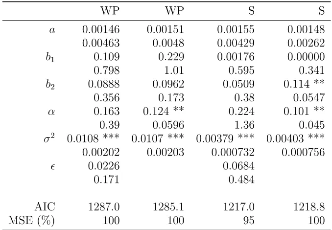
Table 1: Parameter estimates for our pirate model and theǫ = 0restricted model
WP WP S S
a 0.00146 0.00151 0.00155 0.00148
0.00463 0.0048 0.00429 0.00262
b1 0.109 0.229 0.00176 0.00000
0.798 1.01 0.595 0.341
b2 0.0888 0.0962 0.0509 0.114 **
0.356 0.173 0.38 0.0547
α 0.163 0.124 ** 0.224 0.101 **
0.39 0.0596 1.36 0.045
σ2 0.0108 *** 0.0107 *** 0.00379 *** 0.00403 ***
0.00202 0.00203 0.000732 0.000756
ǫ 0.0226 0.0684
0.171 0.484
AIC 1287.0 1285.1 1217.0 1218.8
MSE (%) 100 100 95 100
Standard deviations are shown below the coefficients. *** de-notes an p-value of less than 0.01, ** of less than 0.05, * of less than 0.1. MSEs are expressed as percentages of the MSE for the corresponding restricted model. σ2 is reported in units of 109.
Table 1 shows parameter estimates for our model and its restriction to the Givon et al.
(1995) model. In column one, our model is fitted to the word processor data. The a
parameter equals 0.00146, which is higher than the 0.0002 rate reported in Givon et al.
(1995). Our rates lie between the mean and median of estimates reported in the
(1995) estimate lies at the lower end of their range. Thus, we find that word processors
were subject to external influence to a more usual extent than is found in Givon et al.
(1995) (although the Van den Bulte and Stremersch (2004) data does not disaggregate their reported figure by annual, quarterly, and monthly frequency of calculation, so the
sub-divided ranges may move closer to the Givon et al. (1995) figure). Thus, we find a
higher effect of external influence on diffusion. The b1 parameter equals 0.109, describing
the internal influence on sales by legal owners. The value is lower than in Givon et al.
(1995) where it is 0.135. Our estimate for the pirate internal influence parameter b2 is
0.0888, again lower than in Givon et al. (1995) at 0.135 too. Our α parameter is 0.163,
representing the proportion of internally influenced adopters who buy the legal software
when few past pirate copies have been made. It is higher than in Givon et al. (1995)
(0.144). The σ2 variance parameter is 10,800,000, giving an implied standard deviation
for legal and pirate acquisitions of 3,300 units per month. The ǫ parameter is 0.0226,
indicating that the marginal propensity to pirate rises as the number of pirates rises. This is consistent with a hypothesis that increasing piracy prevalence makes it more viable or acceptable for new adopters to acquire pirate copies. The significance of all parameters is low, except for the error variance.
In column two, we set the ǫ parameter to zero to see how the parameters and fit adjust
compared with the model including it. The parameters on a, b2, and σ2 change little,
although the significance on b2 increases whilst remaining low. The b1 parameter rises to
0.229, with low significance. The α parameter drops to 0.124, and becomes significant at
five percent. The Akaike Information Criterion selects the smaller model over the larger model, and the mean squared errors from the two models are almost identical indicating no in-sample predictive benefit from including the ǫ term.
Column three reports parameter estimates for our model applied to the spreadsheet data. The coefficient of external influence a is 0.00155, similar to that for word processors
and compared to 0.00069 in Givon et al.(1995). The legal owners’ influence parameter b1
is negligible, and far below the external influence parameter b2 of 0.0509. In Givon et al.
(1995), the estimated parameters are larger and comparable at 0.0976 for theb1 parameter
and 0.104 for b2. Our α parameter is 0.224 compared with 0.121 in Givon et al. (1995).
The error variance is 3,790,000 implies a standard deviation for monthly legal and pirate acquisitions of 1,900 units per month. The estimate for the ǫ parameter is 0.0684, so that the marginal propensity to pirate rises with the number of pirates. Except for the variance parameter, significance is low.
Column four shows the model when ǫ is excluded. The a, b1, and σ2 parameters are
The performance of our model vis-`a-vis the restricted model is mixed. Theǫparameter estimates are plausibly positive and low in value. With the word processor data, the extra variable offers no improvement in fit and weakens the significance on theα parameter, but not the other parameters. With the spreadsheet data, there are noticeable gains for the fit, but the parameter significance worsens perhaps indicating that qualitative behaviour of the larger model better describes the data but the functional form is not correctly specified. We examine these issues in the next subsections.
A further notable point is the insignificance of the legal internal influence in any speci-fication. The estimates point to the only possibly statistically significant internal influence coming from past acquirers of pirate copies.
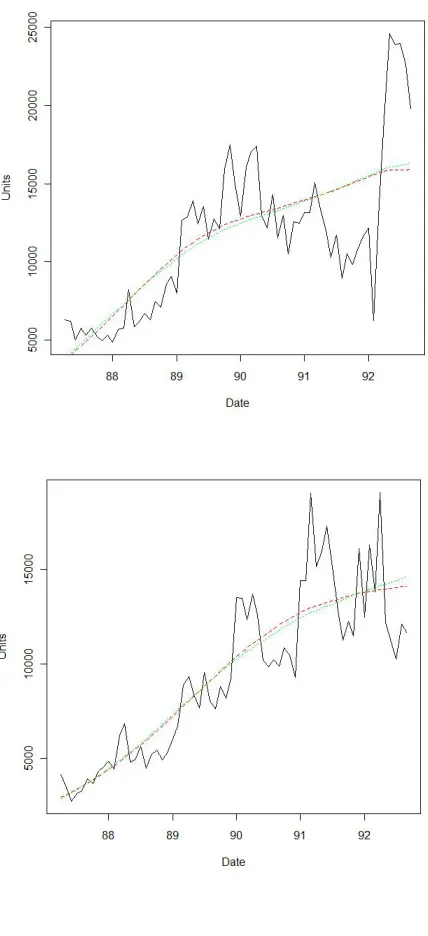
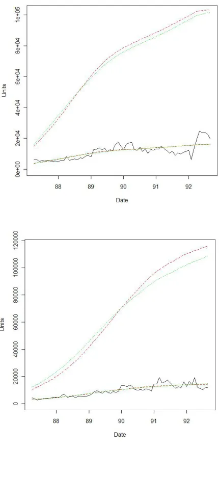
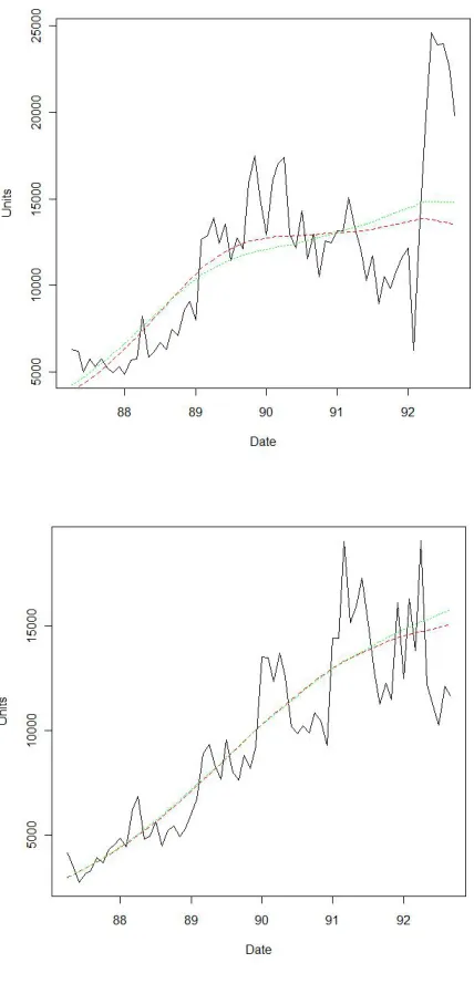
Figure 1 shows the predicted sales as generated by the Kalman filter at our estimated parameters. The top panel shows the fitted sales for word processors in our model (column one in table 1, with red dashes) and in the restricted model (column two, with green dots). Our model fits the data better across most of the period except towards its end where its predictions are lower than the restricted model, and far lower than the suddenly hiked sales. The extra parameter available in our model allows for better fitting but comes at a cost in that pirate sales dominate late in the period, if the optimalǫparameter is positive. The legal sales are lower as a result. In the bottom panel, we see the fitted sales for spreadsheets for our model (column three), and for the restricted model (column four). The fit is comparable between the two models for most of the period, but at the end of the period our model fits much better the sudden fall in sales. The reason for the relative fit is that the extra flexibility in our model allows for comparable fit quality over most of the curve, and then better fit to the late fall as pirate sales displace legal sales. The different directions of the sales shifts at the end of the period explains why the mean squared error for our model with the word processor data is the same as the restricted model, whereas it is much lower with the spreadsheet data.
of the restricted model from early 1990, and the gap is moderately large at high piracy prevalence. The larger gap for spreadsheets than word processors is due to the higher estimated ǫ coefficient for the spreadsheet data.
4.2 Out of sample performance
[image:17.612.123.501.314.537.2]This section compares the predictive performance of our model with that of the restricted model. To do so, we re-estimated our model using data from the first 58 periods, retaining the last ten periods for assessing out of sample fit. For the word processor data, the out of sample period is marked by a large sales jump, while for the spreadsheet data the period saw a possible sales growth slowdown.
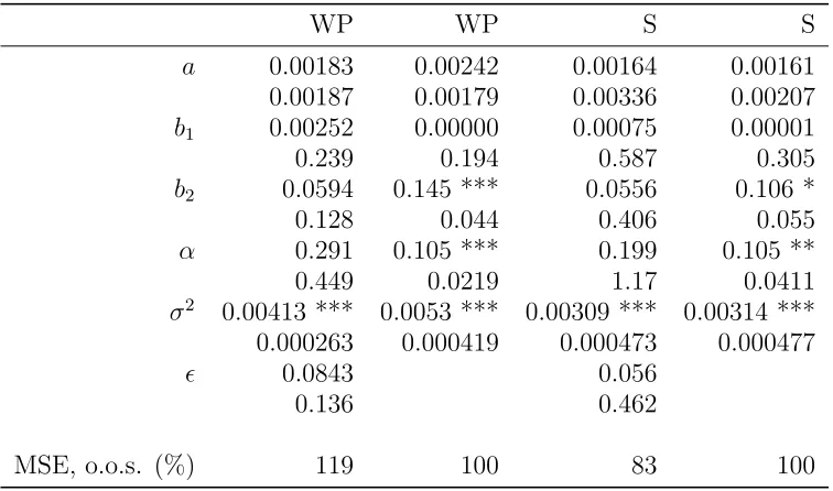
Table 2: Parameter estimates in-sample and MSEs out of sample
WP WP S S
a 0.00183 0.00242 0.00164 0.00161
0.00187 0.00179 0.00336 0.00207
b1 0.00252 0.00000 0.00075 0.00001
0.239 0.194 0.587 0.305
b2 0.0594 0.145 *** 0.0556 0.106 *
0.128 0.044 0.406 0.055
α 0.291 0.105 *** 0.199 0.105 **
0.449 0.0219 1.17 0.0411
σ2 0.00413 *** 0.0053 *** 0.00309 *** 0.00314 ***
0.000263 0.000419 0.000473 0.000477
ǫ 0.0843 0.056
0.136 0.462
MSE, o.o.s. (%) 119 100 83 100
Standard deviations are shown below the coefficients. *** denotes an p-value of less than 0.01, ** of less than 0.05, * of less than 0.1. MSEs out of sample are expressed as percentages of the MSE out of sample for the corresponding restricted model. σ2 is reported in units of 109.
The results are in table 2. Column one shows the estimates for our model applied
to the word processor data. The a parameter of external influence is 0.00183, a little
Figure 3: Predicted and actual sales for word processors (top) and spreadsheets (bottom), with ten out-of-sample periods. Red dashes are for the model with estimatedǫ, green dots are for the model withǫset
far above the whole period value. The variance estimate σ2 is 0.00413, under half of the
full period estimate that includes the sudden sales growth. The estimate of the marginal
propensity to pirate parameter ǫ is 0.0843 compared with the full sample ǫ estimate of
0.0226. The parameter significance is generally low except on σ2, and very low on b 1.
Column two shows similar parameters for the restricted model estimated on the word processor data, without ǫ. The pirate internal influence parameter is fifty percent higher than its full period estimate. The legal share parameter is a little lower. Both these parameters become significant at one percent, unlike the full period estimate or the estimate for the model with variable propensity to pirate.
Our model has a much higher out of sample MSE than the restricted model. Including the variable marginal propensity to pirate worsens fit in this case. The positiveǫcoefficient results in the share of pirate acquisitions rising over time and the share of legal acquisitions falling, which leads to a far better fit than the restricted model over the in sample period (figure 3, top panel). However, the curvature in our predicted sales curve means they lie below the predicted sales of the restricted model after the unprecedented sales jump in the out of sample period.
Column three has the parameter estimates for our model using the spreadsheet data. The external influence, internal legal influence, and legal share parameter are all close to their full period estimates. The internal pirate influence parameter is even smaller than for the full sample, and the error variance parameter is moderately lower. The marginal propensity to pirate parameter is also similar to the value for the whole period, and is positive. Except the variance parameter, significance is low.
The spreadsheet parameter estimates with the ǫ parameter set to zero are in column
four. The estimated volatility is twenty percent lower, but otherwise the parameters are similar to their full period estimates in size and significance.
The mean squared error in spreadsheet sales projection for our model is only 83 percent of the MSE for the restricted model. In our model, the positiveǫparameter means that the share of new piracy rises as the number of past pirates increases, so that legal sales’ share declines. Legal sales are lower in our model than in the restricted model during the sample
period, tracking the decline in actual sales (figure 3, bottom panel). The ǫ parameter is
quite high at 0.056, so that the gap is quite large which accounts for the size of the MSE forecast gain.
The non-additive functional form meant that we could not verify the error correlation assumptions necessary to run Clark-West tests (Clark and West, 2007) of the extra variable offering no predictive gains. When the tests were run under uncertain assumption validity, the null of no gains was rejected at ten percent for spreadsheets (assuming no autocorre-lation in the data). Significance fell a little on allowing for first order autocorreautocorre-lation.
when faced with shocks biased against the general direction of movement. It is unclear, based on the available data, whether such shocks are inherent to the system and occur frequently. If they are and do, then more extensive misspecifications may be preferable to less misspecified models if the partial misspecification decreases predictive accuracy after the shock.
4.3 Alternative error specifications
Our model in equation 2 describes the errors in the legal sales and pirate acquisition series by a bivariate normal distribution. In order to achieve parameter identification, our base
estimations restricted the variance-covariance matrix Q to be a multiple of the identity
matrix. In this section, we compare our estimates under other error specifications.
We consider four Qspecifications, applied to the word processor and spreadsheet series in turn. The first specification puts the variance for the larger pirate series to be twice the variance for the legal series, so q1,1 =σ2 for some constant σ2, q2,2 = 2σ2, and q1,2 = q1,2 = 0. The second specification allows for positive correlation between the legal sales
and pirate acquisitions, setting q1,1 =q2,2 =σ2 and q1,2 =q1,2 =σ2/2. Thirdly, we specify
negative correlation between the two series, so q1,1 = q2,2 = σ2 and q1,2 = q1,2 = −σ2/2.
In the fourth specification, heteroscedastic errors are allowed so q1,1 = q2,2 = Ntσ2 and
q1,2 =q1,2 = 0, recalling that Ntis market capacity at timet, which we express in millions.
Our model was re-estimated with each of these variance specifications. The coefficient estimates are given in Table 3. The word processor results are presented in the first four columns. With doubled pirate variance in column one, the coefficients are similar to the base estimates in value and significance. The marginal propensity to pirate rises a little more quickly. The AIC and MSE are no different. For positive correlation in column two, the estimated effect of legal internal influence is much larger (b1 = 0.334) than in the base model. The marginal propensity to pirate declines as the number of pirate copies rises (ǫ = −0.0147), unlike in the base estimates. The positively correlation provides a route by which pirate acquisitions influence legal sales, and which can therefore account for the diminished importance of the direct influence of piracy on diffusion in this estimation. The AIC is higher for this specification and the mean squared errors are the same.
Column three shows the estimates with negative correlation. Parameter estimates for external influence and variance within series are similar to the base estimate. However, the estimates of the legal internal influence and the legal share parameter are much larger, at 0.381 and 0.226 respectively. Thus, for small timest the proportion of past legal adopters who induce new legal adoptions is 0.381×0.226/Nt = 0.086/Nt. The estimated effect of
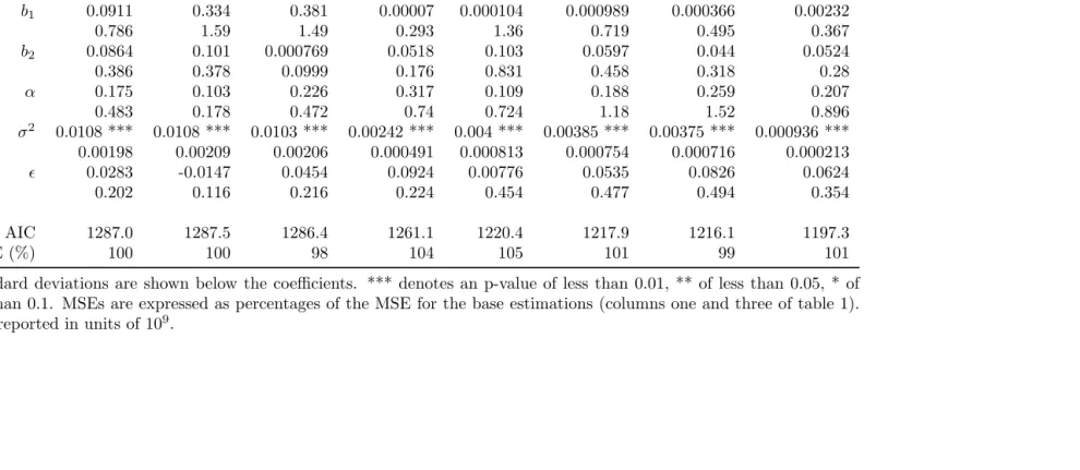
Table 3: Parameter estimates with alternative error specifications
WP WP WP WP S S S S
Err. ×2 Pos. cor. Neg. cor. Het. err. Err. ×2 Pos. cor. Neg. cor. Het. err. a 0.00139 0.00163 0.00123 0.00217 0.00163 0.00161 0.00157 0.00169 0.0046 0.00579 0.00701 0.00163 0.00493 0.00443 0.00407 0.00183 b1 0.0911 0.334 0.381 0.00007 0.000104 0.000989 0.000366 0.00232
0.786 1.59 1.49 0.293 1.36 0.719 0.495 0.367
b2 0.0864 0.101 0.000769 0.0518 0.103 0.0597 0.044 0.0524
0.386 0.378 0.0999 0.176 0.831 0.458 0.318 0.28
α 0.175 0.103 0.226 0.317 0.109 0.188 0.259 0.207
0.483 0.178 0.472 0.74 0.724 1.18 1.52 0.896
σ2
0.0108 *** 0.0108 *** 0.0103 *** 0.00242 *** 0.004 *** 0.00385 *** 0.00375 *** 0.000936 *** 0.00198 0.00209 0.00206 0.000491 0.000813 0.000754 0.000716 0.000213
ǫ 0.0283 -0.0147 0.0454 0.0924 0.00776 0.0535 0.0826 0.0624
0.202 0.116 0.216 0.224 0.454 0.477 0.494 0.354
AIC 1287.0 1287.5 1286.4 1261.1 1220.4 1217.9 1216.1 1197.3
MSE (%) 100 100 98 104 105 101 99 101
Standard deviations are shown below the coefficients. *** denotes an p-value of less than 0.01, ** of less than 0.05, * of less than 0.1. MSEs are expressed as percentages of the MSE for the base estimations (columns one and three of table 1). σ2
is reported in units of 109
.
pirate rises much more quickly in this specification than in the base model (ǫequals 0.0454 compared with 0.0226). The AIC and MSE are lower. In this specification, piracy acts primarily to displace legal diffusion without promoting it.
Column four shows the parameters for the model with heterogeneous errors. Compared with the base model parameters, the external diffusion parameter is moderately larger, as is the estimate of the series error variance. The legal internal influence coefficient is negligible, and the pirate internal influence coefficient is much the same. The marginal propensity to pirate rises much more quickly in this specification (ǫ = 0.0924). The AIC is lower, but the MSE increases by a larger percentage.
Parameter estimates for the spreadsheet data are shown in columns five to eight. The parameters for the double pirate error specification are shown in column five. The external influence and legal internal influence parameters are much the same. The variance coef-ficient is similar at 0.004. The pirate internal influence parameter is almost doubled at 0.103, while the legal share parameter is halved at 0.109. The rise in marginal propensity
to pirate is positive and low, with ǫ at 0.00776 compared with 0.0684 in the base
spec-ification. Significance is generally low, the AIC is higher and the MSE increases by five percent.
In column six, the results are shown for the positive correlation error specification. The parameter estimates are not too dissimilar from the base specification. The AIC and MSE are higher. The parameters for the negative correlation error specification are shown in column seven. The parameters are similar to the base specification, with the marginal propensity to pirate parameter a bit larger. The AIC and MSE are both a little lower. The parameters for the heterogeneous error specification are in column eight. They are again similar to the base specification. The AIC improves by two percent and the MSE worsens by one percent.
In summary, the alternative error specifications broadly support an increasing marginal propensity to pirate. For both the word processor and spreadsheet data, the negative correlation specifications reduce the AIC and the MSE. For the word processor data, the resulting model shows piracy growing rapidly and making little contribution to legal diffusion. Parameter significance is generally low.
4.4 An alternative model
4.4.1 The alternative specification
We noted earlier that our model gives plausible values for the ǫ parameter and some
The alternative specification makes the legal shareαdecline as the number of cumulative pirate adopters rises. The share of new internally influenced adopters who buy is revised toα/(1 + max(Yt,1)ǫ), whereYtis the number of pirates. The remaining share, 1−α/(1 +
max(Yt,1)ǫ), acquires a pirate copy. We omit the piracy multiplier max(Yt,1)ǫ described
in the model in section 2. In the new model, piracy has no accelerating effect unlike the earlier model, and instead only displaces legal sales.
Algebraically, the model is
dXt= (
"
a+1+max(αYt,1)ǫ
b1Xt+b2Yt
Nt
#
(Nt−Xt−Yt))dt+dw1
dYt= (
"
(1−1+max(αYt,1)ǫ)
b1Xt+b2Yt
Nt
#
(Nt−Xt−Yt))dt+dw2
(31)
where dw= (dw1, dw2)∼N(0, dt2Q), and Q=σ2I(2).
We repeat the state space representation in section 3.2.2. Now the vectorf is given by
f1 =
"
a+ α
1 + max(Yt−1,1)ǫ
b1Xt−1+b2Yt−1 Nt
#
(Nt−Xt−1−Yt−1) (32)
f2 =
"
(1− α
1 + max(Yt−1,1)ǫ
)b1Xt−1+b2Yt−1
Nt
#
(Nt−Xt−1−Yt−1) (33)
F1,1 =
"
α
1 + max(Yt−1,1)ǫ
b1 Nt
#
(Nt−Xt−1−Yt−1)
−
"
a+ α
1 + max(Yt−1,1)ǫ
b1Xt−1 +b2Yt−1 Nt
#
(34)
F1,2 =
"
−ǫmax(Yt−1,1)ǫ−1
α
(1 + max(Yt−1,1)ǫ)2
b1Xt−1+b2Yt−1 Nt
+ α
1 + max(Yt−1,1)ǫ
b2 Nt
#
(Nt−Xt−1−Yt−1)
−
"
a+ α
1 + max(Yt−1,1)ǫ
b1Xt−1 +b2Yt−1 Nt
#
(35)
F2,1 =
"
(1− α
1 + max(Yt−1,1)ǫ
)b1
Nt
#
(Nt−Xt−1−Yt−1)
−
"
(1− α
1 + max(Yt−1,1)ǫ
)b1Xt−1+b2Yt−1
Nt
#
(36)
F2,2 =
"
ǫmax(Yt−1,1)ǫ−1
α
(1 + max(Yt−1,1)ǫ)2
b1Xt−1+b2Yt−1 Nt
+ (1− α
1 + max(Yt−1,1)ǫ
)b2
Nt
#
(Nt−Xt−1−Yt−1)
−
"
(1− α
1 + max(Yt−1,1)ǫ
)b1Xt−1+b2Yt−1
Nt
#
4.4.2 Results for the alternative specification
Table 4: Parameter estimates for the alternative model form
WP WP S S
a 0.0016 0.00167 0.00115 0.00135
0.0039 0.00391 0.00525 0.00271
b1 0.167 0.283 0.000853 0.00000
1.27 1.25 0.932 0.551
b2 0.11 0.0857 0.112 0.113
0.237 0.229 0.18 0.0854
α 0.246 0.245 *** 0.33 0.208 **
0.628 0.0947 2.43 0.0903
σ2 0.0108 *** 0.0107 *** 0.00403 *** 0.00407 ***
0.00209 0.00203 0.000827 0.000752
ǫ 0.000467 0.0503
0.326 0.664
AIC 1287.0 1285.0 1220.8 1219.4
MSE (%) 100 100 99 100
Standard deviations are shown below the coefficients. *** de-notes an p-value of less than 0.01, ** of less than 0.05, * of less than 0.1. MSEs are expressed as percentages of the MSE for the corresponding restricted model. σ2 is reported in units of 109.
Table 4 shows the results of estimation for the alternative model. In column one, we see the model fitted to the word processor data. The external influence parameter is 0.0016, comparable with our estimate for our main model. The legal internal influence parameter is
0.167, higher than the main model estimate but comparable with Givonet al. (1995). The
same is true for the pirate internal influence parameter. Theαparameter is larger than for the main model, but the two are not directly comparable. In our model and for low values of the ǫ parameter, the α parameter is twice the legal share. Error variance estimates are unchanged. Theǫparameter is positive, indicating the pirate share of internally influenced adoption rises as the number of pirate copies rises. Parameter significance is low except for variance. Column two fixes the pirate share, and produces almost the same estimates as column two of table 1 whose specification is identical. Differences arise from slight variations in numerical convergence. Including the variable marginal propensity to pirate raises the AIC and does not change the MSE.
influence parameter is comparable with that in the main model, as is the negligible legal internal influence coefficient and the error variance estimate. The pirate internal influence parameter is 0.112, which is twice as high as for the main model and comparable with
Givon et al. (1995). The legal share is 0.165 after adjustment for comparison with the
earlier work, making it lower than in the main model but a little higher than in Givon
et al.(1995). Theǫparameter is moderately positive, indicating rising marginal propensity to pirate. Its significance, as for the other parameters except error variance, is low. As
shown in column four, the model with ǫ set to zero has much the same parameters as
the constrained main model. Its AIC is slightly lower, but has higher MSE than the unconstrained model in column three.
In summary, the alternative model also identifies a rising marginal propensity to pirate in the word processor and spreadsheet data. The model performance is not quite as good as for the main model. Perhaps the acceleration of pirate sales due to piracy, which is present in the main model but missing from this specification, captures an aspect of the data generating process.
5
Conclusion
This paper has examined diffusion of computer software in the presence of piracy. It has generally found that the marginal propensity to pirate rises with the number of past pirate copies. It has found that piracy is responsible for most of the internally influenced diffusion in the spreadsheet market in the period under examination. In the word processor market, an error specification with negative correlation outperformed other specifications and indicated that only legal sales were responsible for internally influenced diffusion.
A number of avenues for future work are suggested. One of them follows from noting that a rising propensity to pirate alters the timing of welfare and profit emergence. Further work could examine their dynamics and strategic behaviour undertaken by legal sellers in order to manage piracy.
Including the marginal propensity to pirate in the pirate diffusion model offers gains in fit and assumption plausibility. However, they were not entirely functionally convincing, with low parameter significance possibly indicating lack of parsimony. Better specifications of the deterministic components of the model could be sought.
Our model’s predictive performance was mixed. It underperformed the restricted model after a large shock contrary to the general sales curvature. Further work could clarify whether these shocks form error corrections to drifts away from the restricted model, or are not systemically related to the models here. In the latter case, analysing the frequency of shocks and their direction would help to clarify the probability and severity of predictive underperformance.
et al. (1995)’s and Haruvy et al. (2004)’s findings on spreadsheets and contradict them on word processors. For the latter point, it is conceivable that the difference between the results is that our allowance of negative error correlation strips out a source of interaction which is forced to be included in the deterministic components of their model. Further work could further distinguish between deterministic and stochastic interactions. It could also allow for serial correlation, for example in a revised state space formulation.
Our work finds contrasting effects of past piracy on the word processor and spreadsheet market. Qualitative studies could examine the reasons for the difference. Conceivably it arises because of the presence of a dominant but declining word processor product (Word Perfect) over the period without an equivalent in the spreadsheet market, or due to different corporate strategies by market leaders.
References
Bass, F. (1969) A New Product Growth Model for Consumer Durables, Management
Science, 15, 215–27.
Basu, A., Basu, A. and Batra, R. (1995) Modeling the Response Pattern to Direct
Mar-keting Campaigns,Journal of Marketing Research, 32, 204–12.
Clark, T. and West, K. (2007) Approximately normal tests for equal predictive accuracy in nested models, Journal of Econometrics, 138, 291–311.
Givon, M., Mahajan, V. and Muller, E. (1995) Software Piracy: Estimation of Lost Sales
and the Impact on Software Diffusion, Journal of Marketing, 59, 29–37.
Givon, M., Mahajan, V. and Muller, E. (1997) Assessing the Relationship between the User-Based Market Share and Unit Sales-Based Market Share for Pirated Software
Brands in Competitive Markets, Technological Forecasting and Social Change, 55,
131–44.
Hamilton, J. (1994) Time Series Analysis, Princeton University Press.
Haruvy, E., Mahajan, V. and Prasad, A. (2004) The Effect of Piracy on the Market Penetration of Subscription Software,Journal of Business, 77, S81–107.
Jain, D. and Rao, R. (1990) Effect of Price on the Demand for Durables: Modeling, Estimation, and Findings, Journal of Business & Economic Statistics, 8, 163–70.
Liu, Y., Cheng, H., Tang, Q. and Eryarsoy, E. (2011) Optimal software pricing in the
Prasad, A. and Mahajan, V. (2003) How many pirates should a software firm tolerate?
An analysis of piracy protection on the diffusion of software, International Journal of
Research in Marketing, 20, 337–53.
R Development Core Team (2009) R: A Language and Environment for Statistical
Com-puting, R Foundation for Statistical Computing, Vienna, Austria,
http://www.R-project.org.
Schmittlein, D. and Mahajan, V. (1982) Maximum Likelihood Estimation for an Innovation
Diffusion Model of New Product Acceptance, Marketing Science, 1, 57–78.
Srinivasan, V. and Mason, C. (1986) Technical Note - Nonlinear Least Squares Estimation
of New Product Diffusion Models,Marketing Science, 5, 169–78.
Van den Bulte, C. and Stremersch, S. (2004) Social Contagion and Income Heterogeneity
in New Product Diffusion: A Meta-Analytic Test,Marketing Science,23, 530–44.
Xie, J., Song, X., Sirbu, M. and Wang, Q. (1997) Kalman Filter Estimation of New Product