Photons in restricted topologies
Kyle Ballantine
A thesis submitted for the degree of
Doctor of Philosophy
Trinity College Dublin
Declaration
I declare that this thesis has not been submitted as an exercise for a degree at this or any other university and it is entirely my own work.
I agree to deposit this thesis in the University's open access institutional reposi-tory or allow the library to do so on my behalf, subject to Irish Copyright Legislation and Trinity College Library conditions of use and acknowledgement.
Kyle Ballantine
Published material
Material from this thesis appears or will appear in the following papers:
K. E. Ballantine, J. F. Donegan, and P. R. Eastham. Conical diraction and the dispersion surface of hyperbolic metamaterials Phys. Rev. A, 90:013803, July 2014.
K. E. Ballantine, J. F. Donegan, and P. R. Eastham. There are many ways to spin a photon: Half-quantisation of optical angular momentum, Sci. Adv. 2, e1501748 April 2016.
Acknowledgements
Firstly I would like to sincerely thank my supervisor, Prof. Paul Eastham, for his help and guidance over the course of this work. He has always been available for lengthy discussions and has constantly challenged me to improve my understanding. I would also like to warmly thank Prof. John Donegan, who got me started in research, and has always been willing to oer guidance when asked. I thank Prof. James Lunney, who has driven work in conical refraction over the years, and Rónán Darcy, who has done much experimental work on the topic. I would like to thank Nigel Carroll and Plamen Stamenov for their assistance with experimental matters. On a more personal level, I would not have reached this stage without the help of many people. My deepest thanks to my parents, who've supported me every step of the way, and to my sister Kelly for many stimulating discussions. Thanks to Noelle, whose love and companionship have been invaluable. To my friends who have helped get me through the tough days, and celebrate the good ones. Leaving many people out, special thanks to Brendan, Tim, Brian, Chuan, and David, who as well as being a friend has taught me much of what I know about research.
Finally I would like to acknowledge funding from the European Regional Devel-opment Fund and the HEA, Ireland.
Summary
In this work we discuss three dierent aspects of the topological classication of propagating beams of light. This topological classication relies on global properties of the light beam, which are insensitive to local disorder or perturbations. However, topological invariants calculated for scalar elds may not fully describe a beam of light, which consists of a vector eld which points in a particular direction at a given time. We consider the extension of the topological classication of light beams to cases where the polarisation is allowed to vary.
When the phase of a scalar electric eld varies around a point, that eld carries angular momentum, proportional to the magnitude of the change of phase. When the polarisation also varies, we show that there is a new angular momentum which is carried by such a beam. This generalised angular momentum accounts for the possible winding in both the direction of polarisation and the phase around a point. We show that the spectrum of this angular momentum can be a half-integer or an integer multiple of Planck's constant.
To conrm these predictions, we measure the angular momentum current in a beam with varying polarisation. As well as the classical current, we measure quantum uctuations due to the discrete nature of the photons which carry this current. This experiment shows that the generalised angular momentum is indeed quantised in half-integer multiples of ~, and provides a general method for sorting
and detecting beams according to their generalised angular momentum.
Next, we study a new class of material, the hyperbolic metamaterial, in the generic case where all three principal dielectric constants are unequal. These mate-rials have negative dielectric constant in one direction, and positive but unequal in the other two. We show that the iso-frequency surface, that is the surface of wave-vectors at which light of a constant frequency can propagate, consists of two sheets which meet at four linear intersection points. We derive a geometrical optics, and then a full diraction theory of light propagating close to one of these directions.
We also include the eects of absorption and discuss how such a material could be realised in practice.
Contents
1 Introduction and motivation 1
1.1 Introduction . . . 1
1.2 Topology and physics . . . 3
1.2.1 General introduction . . . 3
1.2.2 Winding numbers, optical vortices, and topological invariants . 5 1.2.3 Dimension and quantisation . . . 8
1.2.4 Topological invariants and edge states . . . 11
1.2.5 Topological invariants in photonic systems . . . 11
1.3 Conical refraction . . . 13
1.3.1 Paraxial description of conical refraction . . . 15
1.3.2 Gaussian circularly polarised input beam . . . 16
1.4 Outline of thesis . . . 18
2 Generalised angular momentum theory 21 2.1 Introduction . . . 21
2.1.1 Angular momentum of light . . . 23
2.1.2 Angular momentum in two dimensions and the paraxial ap-proximation . . . 26
2.1.3 Operators and eigenfunctions . . . 28
2.1.4 Angular momentum in a conically refracted beam. . . 30
2.2 Generalised angular momentum . . . 31
2.2.1 Introduction to generalised angular momentum . . . 31
2.2.2 Generalised angular momentum: denition . . . 33
2.2.3 Properties and discussion . . . 35
2.3 Generalised angular momentum: measurement . . . 37
2.3.1 Mechanical eects: angular momentum and torque . . . 40
2.4 Quantum uctuations of angular momentum . . . 41
2.4.1 Angular momentum operator . . . 41
2.4.2 Wavepacket states . . . 43
2.5 Calculation of quantum uctuations . . . 45
2.5.1 Orbital angular momentum: coherent states . . . 46
2.5.2 Orbital angular momentum: number states . . . 48
2.5.3 Generalised angular momentum: number states . . . 51
2.5.4 Generalised angular momentum: coherent states . . . 53
2.6 Quantum operators and interferometer . . . 55
2.7 Conclusions . . . 57
3 Generalised angular momentum experiments 59 3.1 Introduction . . . 59
3.2 Angular momentum current and interferometer . . . 60
3.2.1 Shot noise and interferometer output . . . 61
3.3 Varying generalised angular momentum in input beam . . . 62
3.4 Experimental details . . . 63
3.4.1 Dove prisms . . . 63
3.4.2 Interferometer . . . 66
3.4.3 CCD and photodiode . . . 70
3.4.4 Amplier design . . . 71
3.4.5 Measuring shot noise . . . 74
3.5 Classical results . . . 76
3.5.1 Spin and orbital angular momentum . . . 76
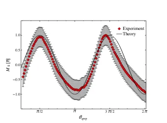
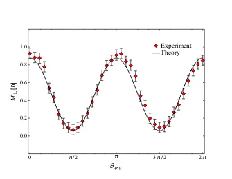
3.5.2 Generalised angular momentum . . . 78
3.6 Quantum results . . . 81
3.6.1 Spin and orbital angular momentum . . . 81
3.6.2 Generalised angular momentum . . . 83
3.7 Error analysis . . . 84
3.8 Conclusions . . . 87
4 Biaxial hyperbolic metamaterials 89 4.1 Introduction . . . 89
4.2 Biaxial hyperbolic metamaterials . . . 91
4.3 Fresnel equation and dispersion surfaces . . . 93
4.3.1 Dispersion surfaces . . . 93
4.3.2 Intersection points . . . 96
4.4 Geometric optics in a hyperbolic metamaterial . . . 98
4.4.1 Refractive index and polarisation . . . 98
4.4.2 Poynting vector . . . 100
CONTENTS xiii
4.5.1 Absorption . . . 102
4.5.2 Diraction . . . 103
4.6 Phase diagrams and possible implementation . . . 106
4.7 Discussion and conclusions . . . 108
5 Gauge elds and topological invariants 111 5.1 Introduction . . . 111
5.1.1 Geometric phase . . . 112
5.1.2 Topological insulators . . . 114
5.1.3 Photonic topological insulators . . . 116
5.2 U(1) invariants in the presence of polarisation coupling . . . 118
5.2.1 Example: chiral biaxial material . . . 118
5.2.2 Homotopies between U(1) vortices . . . 123
5.3 Non-Abelian gauge elds in paraxial optics . . . 123
5.3.1 Calculation of nite operator . . . 126
5.3.2 U(2) topological invariants . . . 127
5.4 Non-Abelian gauge eld of a chiral biaxial material . . . 130
5.5 Conclusions . . . 132
6 Concluding remarks 135
List of Figures
1.1 Illustration of a topological invariant. . . 3
1.2 Example of phase of vortex. . . 4
1.3 Illustration of Gauss's Law. . . 4
1.4 Illustration of homotopy group. . . 6
1.5 Dispersion surface of light in a biaxial medium. . . 14
1.6 Intensity and polarisation of conically refracted Gaussian beam. . . 17
2.1 Schematic illustration of the dierence between spin and orbital angular momentum of light. . . 24
2.2 Spin, orbital and total angular momentum current of conically refracted beam. . . 31
2.3 Illustration of simultaneous rotation of image and polarisation. . . 32
2.4 Illustration of rotation of polarisation ellipse . . . 33
2.5 Polarisation proles of beams with generalised angular momentum. . . . 36
2.6 Illustration of optical sorting and manipulation of generalised angular momentum states. . . 39
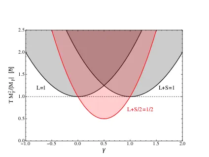
2.7 Normalised noise power in the current of the generalised angular momen-tum Lˆ+γSˆas a function of γ. . . 54
2.8 Illustration of quantum operator formalism for interferometer . . . 55
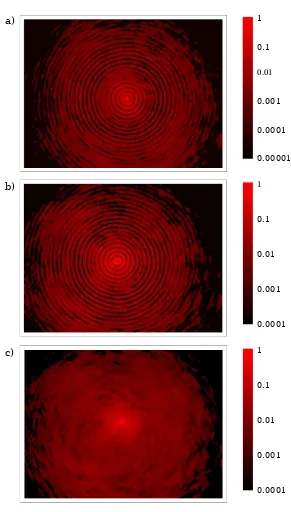
3.1 High dynamic range logarithmic images of Bessel-like beams. . . 64
3.2 Interference patterns showing orbital angular momentum of the compo-nents of the conically refracted beam. . . 65
3.3 Illustration of rays passing through a xed polarisation Dove prism. . . . 65
3.4 Phase of the two orthogonal polarisations due to three reections on passing through the Dove prism, . . . 66
3.5 Illustration of optical sorting of generalised angular momentum states. . 67
3.6 Annotated photograph of experimental setup. . . 69
List of Figures xv
3.7 Scaling of CCD and photodiode response with intensity . . . 71
3.8 Schematic of the electronic equivalent circuit of the photodiode and the designed transimpedance amplier. . . 72
3.9 Transimpedance gain and predicted noise from transimpedance amplier as a function of frequency. . . 73
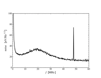
3.10 Measured background noise of transimpedance amplier . . . 73
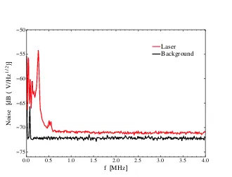
3.11 Intensity noise spectrum of laser . . . 75
3.12 Measured spin angular momentum current . . . 76
3.13 Measured orbital angular momentum current . . . 77
3.14 Images of orbital angular momentum components ltered by interferometer 78 3.15 Measured generalised angular momentum current . . . 79
3.16 Images of generalised angular momentum components ltered by inter-ferometer . . . 80
3.17 Total CCD intensity showing switching between j = 1/2 and j =−1/2 . 80 3.18 Measured Fano factor for spin angular momentum current . . . 82
3.19 Measured Fano factor for orbital angular momentum current . . . 83
3.20 Measured Fano factor for generalised angular momentum current . . . . 85
3.21 Fit of shot noise against DC voltage. . . 86
3.22 Residuals of measured noise from linear t. . . 87
4.1 Example of common hyperbolic metamaterial congurations. . . 90
4.2 Illustration of negative refraction in a hyperbolic metamaterial . . . 90
4.3 Iso-frequency surfaces for dierent possible principal dielectric index signs 94 4.4 Topological transition between Fresnel surfaces describing biaxial mate-rial and biaxial hyperbolic metamatemate-rial . . . 97
4.5 Degenerate points in biaxial material and biaxial hyperbolic metamaterial 98 4.6 Coordinate system for ray description . . . 99
4.7 Poynting vector of conically refracted rays in a biaxial hyperbolic meta-material . . . 101
4.8 Iso-frequency surface in presence of absorption . . . 103
4.9 Full diraction pattern in a biaxial hyperbolic metamaterial . . . 106
4.10 Phase diagram of eective medium theory of silver rods in alumina . . . 107
4.11 Density plots of biaxiality and median index of a biaxial HMM . . . 108
5.1 Illustration of phase depending on path . . . 113
5.2 Energy levels of Hamiltonian Eq. (5.20). . . 120
5.3 Polarisation and instantaneous eld of the eigenvectors of Eq. (5.26). . . 121
5.4 Cross section of Berry ux for lower band of a chiral biaxial material. . . 122
5.6 The four matrix coecients of thexcomponent of the non-Abelian gauge potential A for a chiral biaxial material. . . 130 5.7 The two components of the non-Abelian eld strength F for a chiral
Chapter 1
Introduction and motivation
1.1 Introduction
The behaviour of any physical system is generally described by dierential equa-tions, which can depend in a complex way on many dierent parameters. Usually we can make precise predictions only for idealised systems, ignoring disorder. How-ever, there are properties which cannot be aected by such disorder. For example, consider a knot in a rope which is xed at both ends. This knot cannot come undone, no matter how the rope moves or frays, until the rope breaks completely. Topological properties such as this not only allow for precise characterisation, but also lead to physical laws which, at least in the range of applicability of the theory, are obeyed to an extremely high precision [1, 2, 3].
This topological description of matter leads not only to physical understanding, but also to applications in the design of devices which are insensitive to disorder [3, 4, 5]. The goal of topology in physics is therefore to understand the number of distinct, global arrangements of a physical system, and to use this understanding to design devices which, as long as they remain in one of these arrangements, are constrained to behave in a particular way.
In this work we discuss three aspects of the topological classication of beams of light. Such beams consist of oscillating electric elds which are described at each point by their phase, where in the cycle the eld is, but also by their polarisation, the range of directions in which the eld points over a cycle. While the phase is a crucial property in most topological descriptions of light, the polarisation is often neglected. We focus particularly on the case where this polarisation varies around the beam.
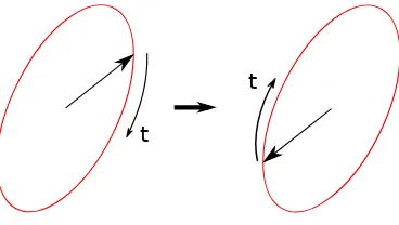
The rst phenomenon we examine, angular momentum of light, concerns beams which are invariant under rotations. If the polarisation is constant, the electric eld can be described by a complex scalar function of time and space, representing both the amplitude and the phase of the oscillation. Clearly for a scalar eld the phase must return to its original value upon traversing a closed loop around the circumference of the beam. Hence, the number of windings in the phase is a xed topological invariant [6, 7]. If the polarisation is also allowed to vary, then the eld is a vector at each point. It may seem that the direction of the eld should also rotate by an integer multiple of 2π. However, the polarisation is dened by an ellipse traced out by the vector eld over one full oscillation. This ellipse is invariant under a π rotation. Hence we can consider in-homogeneously polarised beams, where the phase and polarisation can each rotate by a half-integer multiple of 2π, returning the eld to its original state. We propose a new form for the total angular momentum which allows for the possibility of dierent rates of rotation of phase and polarisation.
The second subject is the iso-frequency surface of a crystal or metamaterial, par-ticularly a hyperbolic metamaterial. It is known that when one dielectric constant of such a material is negative, the iso-frequency surface (the surface of wave-vectors at which light will propagate with a given frequency) undergoes a topological transition from an ellipsoid to a hyperboloid [8, 9]. We extend this to the case of one negative and two positive but unequal constants, and examine the intersections between the hyperboloid and ellipsoid. We derive the ray description of conical refraction in these materials and show that it is topologically and quantitatively distinct from conical refraction in a conventional biaxial material. We also develop a wave optics description, which allows us to obtain the diraction patterns formed from arbi-trary beams incident close to the optic axis. The resulting patterns lack circular symmetry and hence are qualitatively dierent from those obtained in conventional, positive index materials.
The third subject, topological invariants in photonic crystals, is also based on phase winding, this time around a closed loop not in real space, but in reciprocal, or k-space [10]. Here the crystal wave-vector k characterises the solutions of the wave equation in a periodic medium. We show that a new topological invariant, associated with windings in both the phase and the polarisation, is necessary. This invariant may lead to topologically protected edge states in photonic systems (i.e. photonic topological insulators) which are immune to generic, polarisation altering, scattering.
1.2. TOPOLOGY AND PHYSICS 3
topology in condensed matter and in photonics. In section 1.3 we give an introduc-tion to the phenomenon of conical refracintroduc-tion, which results in a beam whose phase and polarisation both vary in space. Such a beam serves as a motivating exam-ple throughout the work. Additional background material on angular momentum, hyperbolic metamaterials, and the topological classication of periodic materials is given in the introduction to each individual chapter.
1.2 Topology and physics
1.2.1 General introduction
a)
b)
c)
Figure 1.1: The familiar topological invariant is the genus of a structure, which counts the number of holes. The sphere a) is genus zero. b) A torus is genus one. c) A more exotic surface with genus two.
Topology is the study of those properties of an object which do not change when the object is smoothly deformed. Smooth deformations can be though of as processes like stretching, twisting etc., but not processes like tearing and glueing. Perhaps the most well-known topological property is the genus, or number of holes an object has. For example a sphere has no holes. It has the same genus as any other such shape; cylinder, cube etc. However a torus, or doughnut shape has one hole, and so is topologically distinct. This concept is illustrated in Fig. 1.1.
Another, related, topological invariant is the phase winding number. Consider a complex scalar eld ψ(~x), i.e. a function which associates a complex number to
each point in space. If we travel around this space in a closed loop, we will arrive back at the same point. However complex numbers are only dened up to a phase of 2π, so eiδ = ei(2nπ+δ). Hence it is possible that over the course of the loop the phase increases by some multiple of 2π. An example is shown in Fig. 1.2, in two dimensions. Following a loop around the center, the phase increases by a total of
-1.0 -0.5 0.0 0.5 1.0
-1.0
-0.5 0.0 0.5 1.0
x
y
Example phase of complex field
-π -π 2
π
2
0
π
Figure 1.2: Example showing the phase (represented by colour) of a eld with a vortex. In this case the phase changes by a total of 6π around the center, so the strength of the vortex is 3. Note the intensity must go to zero at the center of
the vortex, as there is no way to smoothly join up the phase in each direction. Phase dierences of2π are irrelevant, so points which dier by a multiple of 2π are represented by the same colour.
1.2. TOPOLOGY AND PHYSICS 5
If we consider mathematical objects with additional structure, it may not be easy to sort them into dierent categories. Algebraic topology gives a link between global topological descriptions and local, algebraic, ones. A familiar example from physics is Gauss's law. Assuming quantisation of electric charge, the total charge inside a closed surface is a topological invariant. It cannot change smoothly but jumps by a xed amount when a monopole crosses the surface. Gauss's law tells us that this total charge is equal, up to a constant, to the integral of electric ux across the entire surface,
Z ~
E·dA~ =Qenc/0 (1.1)
whereE~ is the electric eld,dA~ a surface element, andQencthe total charge enclosed by the surface. This is a useful example to keep in mind. Locally, the ux through a bit of surface depends on the charge distribution and may not be easy to calculate. However, the total ux is a xed quantity, which cannot be changed by smooth transformations either of the charge distribution, or the Gaussian surface. In the following we will come across examples of complicated local expressions, whose integrals are topological invariants. The local forms of the expressions depend on the particular details of that system, but the invariants capture some simple xed property of the system as a whole.
1.2.2 Winding numbers, optical vortices, and topological
invariants
As we have seen above, surfaces in three dimensions can be characterised by the number of holes. This concept is an important topological property of any space, either real coordinate space or some conguration space of a system. This property is described mathematically by the homotopy group of the space [11]. This group is obtained from the set of all possible closed loops by identifying two loops if one can be smoothly deformed into the other. For example, any loop on the surface of a sphere can be gradually contracted to a point. By contrast, a loop through the center of a torus cannot be contracted in this way. It is the holes in the space which can obstruct these smooth deformations and mean that not all loops are equivalent. This is illustrated in Fig. 1.4 for the example of a sphere and a torus. For a topological description of the space, the placement or size of the hole is irrelevant. What is important is how objects in the space can be congured around it.
Consider a eld whose phase varies with angleφ, for example asψ ∝eilφ with l
an integer. Such a eld could describe a light wave or a quantum wave-function for example. An example is shown in Fig. 1.2, withl= 3. If the eld is continuous, then
a)
b)
Figure 1.4: The homotopy group, which describes how loops can be contracted, gives a mathematical formulation of the concept of the number of holes in a space. On a surface with no holes, such as the surface of a sphere, every loop can be contracted to a point. On a more complicated surface such as a torus, loops around the central hole cannot be contracted. The number of dierent loops which cannot be contracted into each other characterises the surface.
surface) of zero intensity changes the topological nature of the conguration space of the eld. Although the intensity distribution and the phase can be varied around the ring, there is no way to smoothly vary the total phase increase 2πl without breaking the ring of non-zero intensity. This type of phase winding appears in the creation of optical vortices which carry optical angular momentum [12, 13, 14, 15], as well as the topological invariants which are required by phase windings in the Brillouin zone in periodic crystals [10, 16]. In the latter case a gauge transformation, a local redenition of the phase of the eld and the vector potential, which are not independently observable, can be used to move the singularity. However, on a global level the topological charge, i.e. the total number of times the phase changes by2π around the singularity, is unchanged.
Hamilto-1.2. TOPOLOGY AND PHYSICS 7
nian which depends on some set of parameters {λi} such that its eigenvalues and
eigenstates for given parameters are
H(λ)|n(λ)i=n(λ)|n(λ)i. (1.2)
Then as~λis varied in time the states pick up both a dynamic and a geometric phase given by [23]
|n(λ(t))i =eiγn(t)e−i
~
Rt
0n(λ(t
0))dt0
|n(λ(0))i, (1.3)
γn(t) =i
Rλ(t)
λ(0)dλhn(λ)| ∇λ|n(λ)i. (1.4) This Berry phase γ can of course be included in the denition of the states |n(λ)i,
but crucially this can only be done locally. If two dierent paths through the space of possible {λi} give dierent phases, then the dierence does not depend on the
choice of phase; it is gauge invariant. In particular the Berry phase picked up when traversing a closed loop, if it is not zero, cannot be made zero by any consistent choice of phases [23, 24].
In a periodic potential, the wave-functions which satisfy the Schrödinger equation have the form of Bloch waves,
ψ~k(~r) =ei~k·~run(~r), (1.5)
labelled by the crystal momentum k and a discrete band index n. Here un is a
periodic function with the same period as the potential. This is a general result of translation symmetry, and so the electromagnetic modes of a periodic medium have a similar form. As well as the band index n, which is an arbitrary label, each band can be characterised by a topological integer invariant, the Chern number. The Chern number, which is dened precisely below, is a topological number which is similar to the simple count of the number of holes in an object. Intuitively, it counts the number of times the phase of the energy eigenvectors increase by 2π around the edge of the Brillouin zone.
In a periodic medium the Berry phase is a function of the reciprocal momentum ~k. The Berry connection gives the phase dierence between two neighbouring points, and the line integral of this connection gives the Berry phase;
An(~k) =i
D n(~k)
∇~k
n(~k)
E
, (1.6)
γn=
Z
C
d~k· An(~k). (1.7)
Each band is then characterised by the integral of the connection around the edge of the Brillouin zone which, by Stokes theorem, is equal to the integral of the curl of that quantity across the surface of the Brillouin zone [25, 26]:
Cn = 1 4π
I
∂BZ
An(~k)·d~k = 1 4π
Z
BZ
If the phase of the eigenstates n(~k)
E
can be chosen smoothly everywhere then the Chern number will be zero. However, it may happen that this phase cannot be smoothly dened at a number of discrete points. The Chern number simply counts the sum of the phase windings around each of these points, which must be an integer, just as the orbital angular momentum counts the phase winding around the circumference of a beam in real space. A dierent choice of gauge can move these singularities, meaning that the integral around an arbitrary loop is not invariant, but because the Brillouin zone is periodic moving the singularities has no eect and the Chern number is gauge invariant.
An important example of such a topological characterisation of a physical system is the TKNN invariant, named for Thouless, Kohmoto, Nightingale, and den Nijs, of the quantum Hall eect [25], historically one of the rst to be discovered in condensed matter physics. This topological classication explains the plateaus in conductivity of a two-dimensional electron gas in a magnetic eld as a result of an invariant which is conned to be an integer, and so cannot change smoothly. Each occupied band|ujicontributes an integer
nj =
i
2π Z
d~k ∂kxuj
∂kyuj
− ∂kyuj
∂kxuj
(1.9)
to the quantised Hall conductance
σxy =
e2
~
X
j
nj. (1.10)
Since each nj depends on an integral of the curvature of the states over the whole
Brillouin zone, it is a global, topological property of the wave-function.
1.2.3 Dimension and quantisation
Another signicant result of topological considerations which will be crucial to what follows is their role in quantisation. This emerges in lower dimensional systems where the geometry is not sucient to impose quantisation, which arises instead because of global topological requirements. (The dimension, which is often con-sidered as a characterisation of a vector space, is itself more simply a topological property [27].) The restriction to two, one and even zero dimensions has led to many new phenomena in solid state physics [28, 29] and we will see that the paraxial re-striction, from three-dimensional vector elds to two dimensional elds transverse to the propagation direction of a beam of light, leads to new insights into angular momentum.
In three dimensions, quantisation of angular momentum arises as a result of commutation relations
h
ˆ
Li,Lˆj
i
1.2. TOPOLOGY AND PHYSICS 9
where Lˆ is the quantum angular momentum operator rˆ×pˆ. This relation leads to
quantisation by the standard textbook argument [30]. Starting with the eigenstates of Lˆz, considering the eect of the raising and lowering operators Lˆ± = ˆLx ±iLˆy
shows that these eigenstates must be labelled by discrete integers. The commutation relations are geometric constraints, applying equally to innitesimal as well as nite rotations.
In two dimensions, say for a particle constrained to move in the x-y plane, only Lz is non-zero, and so there is no commutation relation to be obeyed. In this case
quantisation comes from the requirement that the eld is single-valued,
ψ(φ+ 2π) = ψ(φ). (1.12)
Assuming that|ψ|is non-zero and thatψ is continuous then the phase must increase by a multiple of 2π around a loop,
Arg(ψ(φ+ 2π))−Arg(ψ(φ)) = 2πl l∈Z. (1.13) This restriction to integer l is therefore a global, topological property [31]. Accord-ingly, the condition Eq. 1.12 does not restrictψ locally. Since the quantisation arises due to topology it is only sensitive to global properties of the space. The simplest function which fulls the requirement in Eq. 1.12 is ψ ∝eilφ.
The global nature of quantisation in two dimensions is the underpinning of the Aharonov-Bohm eect, seen when electrons orbit a solenoid. For an ideal solenoid, the magnetic eld is zero outside of the central core. However, the vector potential is non-zero, and when electrons complete a circuit of a solenoid they pick up a phase proportional to the magnetic ux,
∆φ= eΦB
~ , (1.14)
where ΦB is the magnetic ux through the solenoid [32]. The magnetic ux
punc-tures the space, dividing paths into groups according to how many times they en-circle it. When considering possible orbits of the solenoid, the space is equivalent to a two dimensional plane with the origin removed,R2− {0}. Since every closed path
is characterised by an integer n, the number of times it winds around the solenoid, the homotopy group of this space is the integers Z. This winding leads to a total
This accumulated phase has an interesting implication for the angular momen-tum of two-dimensional particles [33]. In such a system, the restriction Eq. 1.12 will still hold if we demand single-valued wave-functions. However, according to the principle of minimal coupling the magnetic potential must be added to the kinetic momentum to obtain the canonical momentum
~
p=~pcan−q ~A. (1.15)
where q is the charge and A~ is the magnetic vector potential. Hence the angular momentum, which generates rotations [34], is
Lz = (~r×~p)z =−i~∂φ+qAφ. (1.16)
In the simplest single-valued gauge, Aφ= ΦB/2π. The total angular momentum in
units of~ is l−(qΦ/2π~) which is non-integer. This is the most intriguing aspect
of angular momentum in two dimensions: the angular momentum of a particle is not restricted to integer or half-integer values. A modied spin-statistics theorem holds, with interchanged particles picking up an arbitrary phase
|ψ1ψ2i=eiθ|ψ2ψ1i. (1.17)
Such a particle is known as an anyon [34], and obeys so-called "fractional statis-tics", which reduce to Bose-Einstein or Fermi statistics when θ= 0, π, respectively. For example in a strongly correlated electron gas conned to two dimensions, the interaction of each electron with the magnetic eld of all other electrons gives rise to quasi-particles which obey fractional statistics. These have been observed in the fractional quantum Hall eect [35, 36].
An intriguing alternative description is obtained by absorbing the phase picked up upon orbiting the solenoid into a new boundary condition. To do this the mag-netic potential can be removed globally by the transformation
~
A→A~− ∇ΦBφ
2π , (1.18)
which does not aect the magnetic eldB~. However, this transformation is discon-tinuous, for example across the negativex axis if we chooseφ∈(−π, π). This leads
to a boundary condition onψ,
ψ(φ+ 2π) = eiqΦBψ(φ) (1.19)
6
=ψ(φ). (1.20)
1.2. TOPOLOGY AND PHYSICS 11
1.2.4 Topological invariants and edge states
One reason why the topological classication of energy bands is important is the bulk-boundary correspondence. For an insulator with a gap between two sets of bands, the sum of the Chern number, given by Eq. 1.8 , for all bands below the band-gap is a topological property which cannot be changed by smooth deformations [25]. When two such materials, with dierent invariants, are placed in contact, there is no way to smoothly interpolate between the two bandstructures at the boundary without closing the bandgap. Hence the interface between two topologically non-trivial insulators must have conducting states [3, 37, 38]. This relation between a property of the bulk material and its edge states is an example of the bulk-boundary correspondence: the behaviour at the interface between two materials is governed by the topological properties of the bulk bandstructures of each material.
The bulk-boundary correspondence is also responsible for the quantised trans-port in the quantum Hall eect [1, 39]. As remarked in section 1.2.2 there is an integer invariant which characterises each energy band. When the Fermi surface lies between these bands, the bulk material is insulating. However, when there is an interface between such a material and another insulator with a dierent topological classication, then there is no way to smoothly connect the bands across the inter-face without closing the energy gap. This topological requirement leads to at least one conducting state at the edge. The topological necessity of these states explains the remarkable precision of quantum Hall measurements [1], even in the presence of disorder and imperfections which are inevitable in any experiment.
1.2.5 Topological invariants in photonic systems
Topological invariants have been used to classify optical systems, both in real space and reciprocal space. As discussed in section 1.2.2, optical vortices, which exist when electromagnetic elds contain phase windings in real space, have been the subject of theoretical investigation [40, 41, 42]. They have also been used in many applications. Some, such as optical spanners [43, 44], rely on the angular momentum carried in such beams. However, others make use of the topological distinction between dierent vortices, for example to encode information [45, 46]. The discrete nature of the winding number, and the link between topology and quantisation, has also allowed researchers to explore a variety of fundamental quantum phenomena such as entanglement [47], generalised Bell inequalities [48], and the uncertainty principle [49].
are two main ways this has been achieved. The rst is through a direct application of the topological classication of crystal band-structures to the energy bandstructure of photonic systems, for example photonic crystals. The second, less direct, method is to exploit analogies between electric elds and quantum wave-functions, in par-ticular the formal equivalence between the two dimensional Schrödinger equation and the paraxial wave equation [50].
One distinction between fermions and bosons is the nature of the time-reversal operator. This is important because two states can be topologically distinct as long as a particular symmetry is present, but could be deformed into each other through intermediate states which break that symmetry. We will explain in section 5.1, when we discuss topological insulators in more detail, that for fermionic systems there is a class of topological insulators which are protected by time-reversal symmetry. Be-cause the time-reversal operator behaves dierently for fermions than for bosons, time-reversal invariant topological insulators cannot be directly implemented in pho-tonic systems. Time-reversal symmetry can be explicitly broken, for example by including a Faraday material. Such an approach has been shown to lead to topo-logically non-trivial systems [51, 52]. More recently photonic topological insulators have been proposed using metamaterials [53]. In this case the permittivity and per-meability of the metamaterial are tuned to be equal, so the topological classication is protected by electric-magnetic duality rather than time-reversal symmetry.
For a beam of light which consists of rays with small angle to the beam axis, we can make the paraxial approximation, which writes the beam as a plane wave multiplied by a slowly varying envelope function. Under this approximation, the three dimensional wave equation reduces to the paraxial Helmholtz equation
idE dz =−
1 2k∇
2
⊥E. (1.21)
This equation governs the propagation along the beam axis z of the transverse eld. In the case of light in a periodic medium which can be described as a set of weakly coupled paraxial beams, for example a two-dimensional lattice of weakly coupled wave-guides, it may not be necessary to explicitly break time dependence symmetry. The role of time is played by thez coordinate, and z symmetry can be broken by chirality. This has led to topologically protected edge states in a variety of systems [54, 55, 56].
1.3. CONICAL REFRACTION 13
These designs of topological materials without true time-reversal symmetry break-ing rely on decouplbreak-ing between the two polarisation states of light [38]. For example articial gauge elds rely on a change of phase when light of a single polarisation moves around a loop. By overall time-reversal symmetry the opposite polarisation must pick up the same phase when traversing the loop in the opposite direction. Scattering from one polarisation in to the other can therefore lead to losses. In gen-eral scattering from arbitrary defects will not preserve polarisation, and such losses will be inevitable [60], undermining the topological robustness of transport for a single polarisation. Hence it is necessary to understand topological characterisation of beams with inhomogeneous polarisation. This will be the subject of chapter 5.
1.3 Conical refraction
One of our main results is to extend the topological characterisation of optical systems to include cases of inhomogeneous polarisation, i.e. where the ellipticity or the angle of the polarisation varies around the beam, either in real space or in k-space. The motivating example for this extension is the conically refracted beam, which has a polarisation and phase which varies with the azimuthal angle around the beam.
Conical refraction is a phenomenon which occurs in an anisotropic medium with no rotational symmetry. In a general medium the electric eld E~ and the electric displacement eld D~ are related by a tensor
~
Di =ijE~j. (1.22)
Depending on the crystal symmetry ij, in a frame in which it is diagonal, can have
one, two, or three distinct entries, called the principal dielectric constants. A more complete exploration of the resulting crystal optics is given in chapter 4, where we include the possibility of one or more negative dielectric constants. For now we note that for any direction of propagation in a medium, there are two refractive indices given by the Fresnel equation [61]. Depending on ij these two indices may be
equal. For each direction these indices describe the propagation of two orthogonal polarisations. If the two eigenvalues are not equal then the dierent polarisations experience dierent refractive indices, an eect known as birefringence.
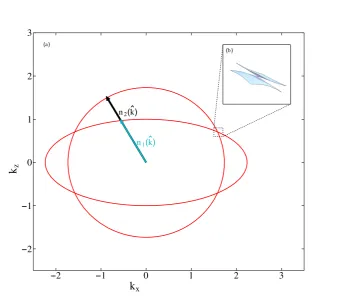
The solutions to the Fresnel equation describe the propagation of plane waves in a particular direction in the crystal given by~k/|k|. These solutions can be visualised
(b) (a)
n1(k)
n2(k)
-2
-1
0 1 2 3
kz
-2 -1 0 1 2 3
[image:30.595.114.453.72.368.2]kx
Figure 1.5: Dispersion surface of light in a biaxial medium. This can be interpreted as a constant frequency surface ω(~k) = ω0 or as a polar plot of the refractive index n1,2 =
~k
/k0 for dierent directions in k-space. The two surfaces give the refractive index for the two orthogonal polarisations. This picture shows that there are four points (directions in k space) where the surfaces intersect, and it is along these directions which conical refraction will occur. (a) Shows a cross section of this surface in the kx-kz plane showing four linear intersections. Inset (b) shows a
close-up of the intersection in three dimensions.
of propagation. For a uniaxial material, with two equal dielectric constants, the refractive indices describing each polarisation are equal in two specic directions and the iso-frequency surfaces intersect quadratically in k-space. However, for a biaxial crystal, with all three dielectric constants unequal, the surfaces intersect at four points, with linear rather than quadratic intersections. These intersections are shown in Fig. 1.5. It is in the direction of these intersections which beams undergo conical refraction.
Conical refraction, rst predicted by Hamilton and subsequently observed by LLoyd in 1832, is an interesting phenomenon of singular optics. The normal to the iso-frequency surface, which usually gives the direction of the Poynting vector asso-ciated with each ray [61], is not well dened at the linear intersection point. The only restriction on the direction of the Poynting vector is that it must be perpendic-ular to the electric eldE~ and the magnetic eld H~. Similarly D~,B~ =µ
1.3. CONICAL REFRACTION 15
take values given by −1D~. The Poynting vector will take values perpendicular toE~ and B~, which lie along a cone skewed away from~k. Thus a single ray of unpolarised or circularly polarised light will be refracted into a cone. Polarisation singularities of this type occur generically when the isotropic symmetry of vacuum is broken [62]. Although the main theory of conical refraction has long been established it re-mains an active area of research. Conical refraction has been utilised for applications such as optical trapping [63, 64, 65] and lasing [66]. Recently the conical refraction of non-Gaussian beams has been explored experimentally [67, 68]. As we will de-scribe in chapter 2, the conically refracted beam also has a unique optical angular momentum distribution [69, 70].
1.3.1 Paraxial description of conical refraction
Since the conical diraction beam will be used as the main example throughout this work, as well as in the experimental measurements in chapter 3, we now present a brief overview of the paraxial theory which describes such a beam. This treatment follows Berry [71], although the original formulation of conical refraction is due to Belskii and Khapalyuk [72, 73]. The solution of the paraxial wave equation in a biaxial medium is given by the evolution along the beam axis, taken to be the z axis, as a function of the orthogonal coordinates R~ = (x, y), of an initial electric eld. This initial eld evolves under a paraxial Hamiltonian
~
E(R, z~ ) = exp
−ik Z z
0
dz0H(P , z~ 0)
~
E(R,~ 0), (1.23)
where
H = 1
2P
2+AP cosθp sinθp
sinθp −cosθp
!
, (1.24)
= 1 2P
2+A ~P ·~σ. (1.25)
Here k0 is the vacuum wave-vector ω/c, A is a measure of the biaxiality, k =n2k0 where n2 is the median refractive index (i.e. n1 < n2 < n3, ni =
√
i), P, θp are
circular coordinates of the relative transverse wave-vector P~ = (kx, ky)T/k
0, and
~
σ = {σ3, σ1} is the two-dimensional vector of Pauli matrices in a Cartesian vector basis. The unitary operatorexp−ikR dzH evolves the beam forward along thez axis according to the paraxial wave equation,
−i∂ ~E
∂z =H ~E, (1.26)
If the incident beam is uniformly polarised, with polarisation Jones vector eˆ0, and circularly symmetric, then Eq. 1.23 can be written as
~
E(R, z~ ) =
"
B0(R, Z) +B1(R, Z)
cosθr sinθr sinθr −cosθr
!#
ˆ
e0. (1.27)
The coecientsB0 and B1 are integrals over Bessel beams given by
B0 =k R∞
0 dP P a(P) exp(−ikZP
2/2) cos(kR
0P)J0(kRP), (1.28) B1 =k
R∞
0 dP P a(P) exp(−ikZP
2/2) sin(kR
0P)J1(kRP), (1.29) and a(P) is the circularly symmetric Fourier transform of the incident eld,
a(P) =k Z ∞
0
dR RE0(R)J0(kRP). (1.30)
Here for simplicity Z is a re-scaled z coordinate Z = l+ (z −l)n2 where l is the length of the crystal, and R0 = Al. Hence a uniformly polarised input beam is converted into two components. The rst retains the original polarisation and the other, with a dierent spatial distribution, has its polarisation altered in a position dependent way.
1.3.2 Gaussian circularly polarised input beam
Of particular interest is the case of an incoming Gaussian beam with circular polar-isation;
a(P) = kw2exp −k2P2w2/2, (1.31)
ˆ
d0 = (1,±i)T. (1.32)
As explained further in section 2.1.2, the Jones vectors (1,±i)T correspond to left
and right circularly polarised light respectively. In this case the matrix which ap-pears in Eq. 1.27 both interchanges the circular polarisations and also adds a position dependent phase
cosθr sinθr sinθr −cosθr
!
1
±i !
=e±iθ 1
∓i !
. (1.33)
Hence the two polarisations from each term of Eq. 1.27 add with dierent phases at each point. Of particular importance is the focal image plane Z = 0, which would
1.3. CONICAL REFRACTION 17
ρ0
(a)
ρ
yρ
x(b)
ρ
yρ
x(c)
0 5 10 15
Z
/
kw
2
-1 0 1
ρ
x/ρ
0under propagation along the z axis. Figure 1.6(b) shows the polarisation around the beam in the focal image plane. The arrows show the instantaneous eld at a xed time, illustrating the phase. The polarisation rotates by 180◦ around the
circumference of the beam.
1.4 Outline of thesis
In this thesis we consider the spatially varying phase and polarisation of beams like those arising from conical refraction as the starting point for the investigation of inhomogeneous polarisation in several dierent contexts. This leads to extensions of the theoretical description of angular momentum of light, hyperbolic metamaterials, and topological invariants of photonic systems, in order to account for winding polarisation as well as phase.
In chapters 2 and 3 we show that there is a new class of angular momentum oper-ators, which we refer to as generalised angular momentum. Chapter 2 provides the theoretical foundation of this generalised angular momentum. We derive the clas-sical properties of this quantity and also obtain the associated quantum operator. The angular momentum is shown to have an appropriate mechanical eect in sec-tion 2.3. The quantum uctuasec-tions in the angular momentum of both number and coherent states carrying generalised angular momentum are derived in section 2.4.
In chapter 3 we report a series of experiments to measure the generalised an-gular momentum, using a Mach-Zehnder interferometer which performs phase and polarisation rotations on the light in one arm relative to the other. We describe the experimental method in detail in section 3.4. We have measured the spin, or-bital and generalised angular momentum current for various beams with the results given in section 3.5. The shot noise in the angular momentum current, which reveals the quantum of angular momentum, was also measured for spin, orbital and gen-eralised angular momentum. The results, which show that the gengen-eralised angular momentum in a coherent beam may be carried in half-integer multiples of Planck's constant, appear in section 3.6.
In chapter 4 we extend the theory of conical diraction to a new context, that of a hyperbolic metamaterial with at least one negative dielectric constant. We describe the topological change of the refractive index surface from ellipsoid to hyperboloid in section 4.3, and derive both the geometrical optics description (in section 4.4) and the full diraction theory (in section 4.5) of light propagating close to an intersection of that surface.
1.4. OUTLINE OF THESIS 19
describe bands with varying polarisation as well as phase. In section 5.3 we show that a non-Abelian gauge eld describes these bands, and that there is an integer topological invariant associated with this eld. We derive simple formulas to cal-culate this eld and the invariant in the presence of polarisation coupling. Finally in section 5.4 we illustrate these results by applying them to an example of a chiral biaxial material.
Chapter 2
Generalised angular momentum
theory
2.1 Introduction
In this chapter we turn to the rst of the three subjects which we deal with in this thesis; angular momentum of light with inhomogeneous polarisation. This chapter consists of a theoretical exploration of a new quantity, which we call the generalised angular momentum. In chapter 3 we will turn to experimental measurements of the classical mean and the quantum uctuations of this quantity for varying beams of light.
In general, the angular momentum carried by a beam of light can be decomposed into two contributions. The rst is spin angular momentum, due to the rotation of the electric eld vector at each point in space [74]. The second is the orbital angular momentum [17], due to varying phase around the beam as a whole, leading to an azimuthal component of the wave-vector. In three dimensions these two quantities combine equally to form the total angular momentum [75].
Eects due to the angular momentum of light have been studied since the rst measurements of the torque exerted by beams of polarised light, and versions of those mechanical eects appear in experiments on optical trapping and manipulation [76]. Angular momentum eects are also emerging in the radio-frequency domain, for applications in astronomy and communications [45]. Fundamental interest focuses on the photon's angular momentum as a quantum-mechanical property [77]. The angular momentum of single photons has been measured [78], and entanglement [41] and EPR-like correlations [47] studied.
Many of these applications use either the spin or the orbital angular momentum independently, rather than the total angular momentum. This is possible because most laboratory beams are composed of rays at small angles to the beam axis. Such beams can be approximately described by the two dimensional eld transverse to the beam axis. In this case the spin and orbital angular momentum are both physical [79, 42], and we can consider other quantities besides their sum.
If the electric eld at a particular point in the beam does not have equal ampli-tude in all directions, then the electric eld vector traces out an ellipse as it rotates, rather than a circle. The eld is specied by the phase at each point, but also by the angle of the major axis of this ellipse. We will show that when this angle is allowed to vary in space then there is a generalised angular momentum which de-scribes such beams. This generalised angular momentum is a linear combination of spin and orbital angular momentum with either integer or half-integer coecients. Furthermore, the eigenvalues of this angular momentum can be half-integer as well as integer, leading to a value of angular momentum per photon which is a fractional multiple of Planck's constant. Fractional electronic charge and angular momentum has previously been observed by demonstrating a reduced shot noise in an elec-tronic current [80]. Our results open the way to experiments studying fractional quantisation using photons in place of electrons [81, 82, 83, 84].
2.1. INTRODUCTION 23
2.1.1 Angular momentum of light
The mechanical properties of light were rst explored by Poynting, concentrating on linear momentum. The Poynting vector [85] is the cross product of the electric and magnetic elds, and is proportional to the momentum density (momentum per unit volume) of an arbitrary electromagnetic eld
~
P =0E~ ×B.~ (2.1)
This linear momentum density is conserved in any medium with translation invari-ance, and can be measured in a variety of ways, for example by the pressure that a beam of light exerts when reecting from an object [86].
In analogy to classical mechanics, we can dene an angular momentum density which is simply the cross product of position with momentum. The total angular momentum is then
~ J =
Z
d3r 0~r× h
~ E×B~
i
. (2.2)
This quantity is also conserved in a rotationally symmetric medium, and is known as optical angular momentum [85, 87]. In the presence of charged matter Eq. 2.2 contains contributions from longitudinal elds, i.e. electric elds which are parallel to the linear momentum density, at any point. These are due to the Coulomb forces between particles, and can be grouped with the angular momentum of the particles themselves. The contributions from the transverse elds are characteristic of propagating light [75]. In the following we will concentrate on the propagating part, due to the transverse elds, and ignore the possibility of free charges.
The magnetic eld of a propagating wave can be described by a gauge dependent magnetic potential A~ such that B~ = ∇ ×A~. Using the part of the vector poten-tial which is transverse to the linear momentum at each point A~⊥, which is gauge invariant, and the transverse electric eld E~⊥, the total angular momentum can be written suggestively as J~=~L+S~ [88, 75] where
~ S =0
Z
d3r ~E⊥×A~⊥, (2.3)
~ L=0
Z
d3r ~E⊥·(~r× ∇)A~⊥, (2.4)
Although this interpretation in terms of spin and orbital angular momentum is not without problems [75, 79], the spin angular momentum associated with circu-lar pocircu-larisation has long been known. It was rst demonstrated by Beth [90] by measuring the torque produced by circularly polarised light on a wave-plate. The polarisation of the light can be expressed in the basis of right and left circularly polarised light. In each of these states the electric eld vector rotates clockwise or counter-clockwise as the beam propagates leading to an angular momentum of ~
or −~ per photon. This angular momentum is due to a rotating electric eld, as
illustrated in Fig. 2.1(a).
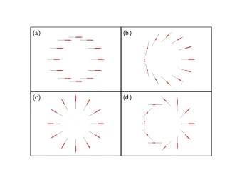
Figure 2.1: Schematic illustration of the dierence between spin and orbital angular momentum of light. (a) Spin orbital angular momentum can be pictured as a rota-tion of the vector polarisarota-tion in time, at each point in space. (b) Orbital angular momentum, due to the changing phase around the beam, can be pictured as the whole beam rotating about its centre. The intensity must be zero at the centre of the beam, as the phase is not dened.
The orbital part of the angular momentum is associated with light beams whose phase depends on the azimuthal angle around the beam. Vortices in waves such as light were rst identied in 1987 [62]. The simplest example is a eld which is proportional toeilφwherelis an integer to ensure the eld is single-valued [91]. The wave vector then has an o-axis component which spirals around the beam. This can be pictured as rotation of the beam as a whole around its centre. Each photon carries l~, an integer multiple of Planck's constant, of orbital angular momentum. This type of angular momentum of light is illustrated schematically in Fig. 2.1(b).
The average angular momentum per photon,±~for circularly polarised light and
l~for orbital angular momentum states, can be calculated classically as the angular momentum per unit energy, multiplied by ~ω [92]. However, these considerations
2.1. INTRODUCTION 25
each of which has a denite orbital and spin angular momentum. These have the form [87];
ul,p(r, φ, z) =eilφfl,p(r, z), (2.5) where l is an angular index,p a radial index which will be suppressed, and
fl,p(r, z) =Cple−r
2/w2
e−i(2p+|l|+1) atan(z/zr)(−1)p(r√2/w)|l|L|l|
p (2r
2/w2). (2.6)
Here Cpl, w, and zr are constants which characterise the beam and p and l are
integers. The Laguerre-Gauss modes are orthonormal when integrated over the plane transverse to the beam axis,
Z
d2r ul,p(~r⊥)ul0,p0(~r⊥) = (2π)2δl,l0δp,p0, (2.7)
and complete, i.e. any transverse eld can be expanded as a linear combination of these modes [94].
The quantisation is done by expanding the eld in these modes [95, 96],
~
E =X
l,σ
al,σuleσ+a∗l,σu
∗
leσ, (2.8)
with e±1 representing the right and left circular spin basis. The expansion coe-cients are then promoted to operators and commutation relations imposed (a process known as canonical quantisation);
al,σ →ˆal,σ,
h
ˆ
al,σ,ˆa
†
l,σ0 i
=δll0δσσ0.
(2.9)
This expansion can then be substituted into the classical expression for other quan-tities. In particular, the angular momentum observables, which are now operators, have a simple form;
ˆ
L=Xl~a†l,σal,σ, ˆ
S =Xσ~a†l,σal,σ, ˆ
J = ˆL+ ˆS.
(2.10)
This is just the number of photons in each mode, times the angular momentum of that mode, summed over all modes [96]. We will return to the quantum optics of angular momentum in section 2.4.
The interpretation of Eq. 2.2 as the sum of separate spin and orbital angular momentum given by Eqs. 2.3 and 2.4 has been controversial. It has been found [79] that the total orbital angular momentum can depend partly on polarisation, while the spin angular momentum can also depend on the azimuthal phase. It has also been shown that the quantum operators Lˆ and Sˆ are not true angular momenta as
This is a consequence of expanding the eld in a set of transverse modes. Rota-tions that act on the eld and not the coordinate basis, or vice versa, do not gener-ally preserve this transversality. Hence only the combination Lˆ+ ˆS corresponds to
angular momentum in three dimensions [95].
2.1.2 Angular momentum in two dimensions and the
paraxial approximation
To be more precise, the reason why L~ and S~, and their corresponding quantum operatorsLˆ andSˆ, are not proper angular momenta, and the root of the diculties
with this interpretation, is that they do not generate the correct algebra,so3. This is the algebra of innitesimal rotations, which generate nite rotations in three dimensions, given by the group SO(3). This group can be represented by special
orthogonal 3×3 matrices and is non-Abelian. These full rotations of the
three-dimensional eld would indeed preserve transversality. The structure ofso3, encoded in the commutation relations Eq. 1.11, leads to a particularly constraining form of the spin-statistics theorem which classies particles as bosons with integer spin or fermions with half-integer spin [97, 98].
The subject of angular momentum in two dimensions is considerably simpler. In two dimensions the relevant group isSO(2)which is Abelian. This results in a trivial
algebra whichLz andSz do obey. It also means that particles can have an arbitrary
quantum spin which need not be an integer or half-integer multiple of Planck's constant. As described in section 1.2.3, a modied form of the spin-statistics theorem relates the phase when two particles are interchanged to the fractional angular momentum. Particles with fractional angular momentum in two dimensions are called anyons [33].
Although light in general is described by a three dimensional vector eld, the description of propagating beams can be simplied by considering only rays which propagate at small angles to the z-axis. The total eld can be written as a plane wave times a slowly varying envelope function,
~
ETOT = Re h
ei(kzz−ωt)E~
i
, (2.11)
with kz = 2π/λ. The eld is then described by a two dimensional complex vector,
e.g. E~ = (Ex, Ey)T in a Cartesian basis. The Helmholtz wave equation ,
∇2− 1 c2
∂2 ∂t2
~
ETOT = 0, (2.12)
then leads to the paraxial wave equation
∇2
⊥+ 2ikz
∂ ∂z
~
2.1. INTRODUCTION 27
under the approximation that
∂2E~ ∂z2 kz
∂ ~E ∂z , (2.14)
i.e. the envelope function varies slowly compared to the wavelength of the light. The dierential operator ∇2
⊥ = d2x +d2y is the transverse part of the Laplacian.
Equation 2.13 is equivalent to the two dimensional Schrödinger equation with the beam axis coordinate z playing the role of time [50]. As with the Schrödinger equation, in more complex systems with inhomogeneity, anisotropy, etc. we can derive a paraxial equation similar to Eq. 2.13 but with more terms added to the Laplacian operator which describes light in free space. We have already seen one such example describing light in a biaxial medium in section 1.3.1.
The complex two-dimensional vectorE~, known as the Jones vector, encodes both the phase and the polarisation of light. For example the circular polarisation states are represented by
|Li= 1
i !
, |Ri= 1
−i !
, (2.15)
which according to Eq. 2.11 gives
~ ETOT =
cos(kzz−ωt)
±sin(kzz−ωt)
!
. (2.16)
This reduction to a two-dimensional transverse eld simplies many of the prob-lems with interpreting angular momentum in three dimensions. In particular the quantum versionsLˆz and Sˆz can be considered angular momenta, since they respect
the trivial algebra of so2. Secondly, in the paraxial picture there is a well dened beam direction, and it is natural to consider the angular momentum current across a plane perpendicular to this direction. This is dened as
M =
Z
d2r 0
~
r×hE~ ×B~i·ˆez, (2.17)
where the integral is over the x-y plane. This current has units of angular mo-mentum per unit length along the beam axis. Because we are using the paraxial approximation, the plane wave part of the eld in Eq. 2.11 depends on the com-bination z−ct, and it can be shown that the angular momentum per unit time is simply given by cM [42].
It can be shown [92, 42] that in the paraxial approximation the angular momen-tum currents can be written as
ML= Re
0c
2ω Z
d2r ~E∗·
−i d dφ ~ E , (2.18)
MS = Re
0c
2ω Z
d2r ~E∗σ3E~
where in Eq. 2.19 we write E~ in a circular polarisation basis. When M is written as ML +MS the current separates into components which depend only on the polarisation and the orbital structure of the beam respectively [42].
The total angular momentum current in a beam with a particular phase or polarisation prole will depend on the total intensity of the beam. We can normalise Eq. 2.19 by the total energy ux to give the angular momentum per unit energy. Furthermore, multiplying this quantity by~ωgives the average angular momentum
per photon;
J =L+S = Re~
R
d2r ~E∗ ·(−idφ+σ3)E~ R
d2r ~E∗·E~ . (2.20)
It should be kept in mind however, that despite the appearance of~this is a purely
classical result.
2.1.3 Operators and eigenfunctions
As the two-dimensional transverse eld transforms under the Abelian rotation group SO(2), we wish to explore the possible form of the total angular momentum operator
for photons in a paraxial beam of light, specied by a two component complex vector eld E~. We take circularly polarised states as our basis and use polar coordinates
(r, φ) across the beam. The angular momentum operators involve the innitesimal
generators of rotations that act on this eld. They include [92] the third Pauli matrixSz =~σ3, which rotates the polarisation direction homogeneously across the beam, and the usual orbital formLz =−i~I(d/dφ), which rotates the beam prole
but leaves polarisation unchanged (noteσ3is the equivalent in a circular polarisation basis of σ2 in a Cartesian one).
To show that these are the operators which generate rotations, consider innites-imal rotations of the eld [92, 40]. The orbital operator follows from
~
E(φ)→E~(φ+δφ), (2.21)
≈E~ +δφd ~ E
dφ, (2.22)
=
1 +δφ d
dφ
~
E, (2.23)
so that
L=−i d
dφ. (2.24)
2.1. INTRODUCTION 29
the Cartesian basis of linear polarisations, E~ = (E
x, Ey)T, we have
~
E → cos(δφ) sin(δφ), −sin(δφ) cos(δφ)
! ~ E,
≈ 1 δφ −δφ 1
! ~ E,
= (I+iδφσ2)E,~
(2.25)
and the spin operator is the second Pauli matrix σ2. This becomesσ3 on transform-ing to the basis of circular polarisations. The factor i is inserted to be consistent with the usual convention relating elements of the group to the generators, i.e. X = exp(ixδφ)≈(1 +ixδφ).
These operators, which form the Lie algebra of innitesimal rotations, generate the Lie group of nite rotations through exponentiation,
RL(φ0) = exp(iφ0L), (2.26) RS(φ0) = exp(iφ0S). (2.27) The operatorsLandSare exactly those which appear in the classical expressions for the expectation value of angular momentum of a beam [92, 42] given by Eq. 2.19
M = 0c 2ω
Z
d2r ~E∗
−i d
dφ +σ3
~ E
= 0c 2ω
Z
d2r ~E∗[L+S]E.~
(2.28)
These expressions are identical to those which describe the expectation value of a quantum operator, if we were to interpret the eld E as a wave-function. This is a consequence of the identical form of the paraxial wave equation Eq. 2.13 and the two dimensional Schrödinger equation [50, 99]. However, at this stage they should be interpreted as purely classical expressions. The inherently relativistic nature of propagating light elds means they cannot be treated in a rst-quantised theory.
However, the operators are clearly linked to the full second quantised expres-sions. Expanding the eld in a complete set of eigenmodes of L and S, {Fl,σ},
and quantising leads to the quantum spin and orbital angular momentum opera-tors [95, 96],
ˆ
S =X
l,σ ˆ
a†l,σˆal,σhFl,σ|S|Fl,σi, ˆ
L=X
l,σ ˆ
a†l,σˆal,σhFl,σ|L|Fl,σi.
(2.29)
This process leads for example to Eq. 2.10 when the elds F are Laguerre-Gauss modes. Note that here Lˆ and Sˆ act on the quantum state of the electromagnetic
used to represent the eld purely for ease of notation). In this representation each photon contributes an exact amount of both spin and orbital angular momentum. When the eld is in an eigenmode of the operators then all photons will be in the same angular momentum mode and so carry an exact amount l or σ of orbital or spin angular momentum.
In this chapter we will frequently refer to beams which are symmetric under a particular rotation. By this we mean that the beam is invariant up to a phase. Conservation of an angular momentum corresponds not to a particular property of the beam, but to the invariance of the medium to such a transformation. The reasons for considering beams which are eigenstates of a particular angular momentum are two-fold. Firstly, if a particular medium respects a symmetry, then eigenstates will remain eigenstates as they propagate, while other states will be mixed. Thus, so long as the states form a complete basis, the propagation of any beam can be described by the propagation of its components in that basis, each of which simply picks up a dierent phase. We can also describe the eect of optical devices, etc. by their eect on each eigenmode. Secondly, although invariance of the medium guarantees the conservation of the classical expectation value, the photons in a beam which is a mode of the operator will have an exact value of that quantity, while other beams will consist of photons which are in a superposition of dierent states, and so do not have a well dened exact value. As the Laguerre-Gauss beams do for orbital angular momentum, the eigenmodes of a particular angular momentum give us a basis to explore the properties of that angular momentum both theoretically and experimentally.
2.1.4 Angular momentum in a conically refracted beam.
The conically refracted beam described in chapter 1 has a unique angular momentum distribution [71, 69]. Equation 1.27 shows that incoming light with circular polari-sation (i.e. spin angular momentum) is converted into light with a combination of spin and orbital angular momentum,1
±i !
→B0
1
±i !
+B1e±iφ
1
∓i !
, (2.30)
or in terms ofl and s
|l = 0, s=±1i →B0|l= 0, s=±1i+B1|l =±1, s=∓1i, (2.31) whereB0 and B1 are given in Eq. 1.28. One component has the same spin angular momentum as the incident beam while the other component has the opposite spin angular momentum and also has orbital angular momentum l = ±1. Thus the
2.2. GENERALISED ANGULAR MOMENTUM 31
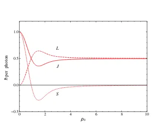
L
J
S
-0.5 0.0 0.5 1.0
ℏ
per
photon
0 2 4 6 8 10
[image:47.595.145.478.71.322.2]ρ0
Figure 2.2: Spin, orbital and total angular momentum, per photon, of conically refracted beam as function of crystal strength parameter ρ0. Note fractional values are just average classical values due to beam being in a superposition of dierent states. Based on an identical gure in [6