Bottlebrush Block Polymers: Molecular
Architecture and Materials Design
Thesis by
Alice B. Chang
In Partial Fulfillment of the Requirements for the Degree of
Doctor of Philosophy
CALIFORNIA INSTITUTE OF TECHNOLOGY Pasadena, California
2018
2018
Alice B. Chang
ACKNOWLEDGMENTS
This thesis represents contributions from many people, including mentors, colleagues, family, and friends. Our interactions have shaped me into the scientist and person I am today, and I would like to thank everyone for their support over the years.
I would first like to thank my advisor, Prof. Bob Grubbs. Bob has been a great mentor, and it has been a great privilege to work in his group. One of the lessons Bob teaches is simple but empowering: don’t be afraid to learn new things. Bob communicates this through his diverse interests and generous support, which have enabled us to pursue the work described in this thesis at the intersection of polymer chemistry and polymer physics. The tremendous depths of Bob’s creativity, curiosity, and kindness are truly inspiring. Moving forward, I can only do my best to live up to his support and his example.
I would also like to thank the members of my committee: Profs. Dave Tirrell, Dennis Dougherty, and Zhen-Gang Wang. Our conversations and committee meetings have been wonderful opportunities to discuss research directions and explore new ideas. I greatly appreciate their support and insight.
I would next like to thank other members of the Caltech community, starting with the Grubbs group. Thank you for being awesome friends and labmates! Whether we’re sharing ideas, chemicals, or memes, you’ve made the lab a fun and inspiring place to work. I would especially like to thank three former colleagues with whom I worked closely: Drs. Garret Miyake, Chris Bates, and Tzu-Pin Lin. Their creativity, expertise, and encouragement have deeply influenced the way I do and think about science.
I started to work with Chris during my first year as a grad student, shortly after Chris joined the group as a postdoc. Chris introduced me to polymer physics, and we worked together on several aspects of this thesis, including the phase behavior of low-χ block polymers (Chapter 4) and brush polymer electrolytes (Chapter 6-2). Working with Chris taught me many valuable skills, including how to finish a project and how to write a paper, as well as the value of building diverse interests. At any point, Chris may be reading a textbook on X-ray diffraction or statistical thermodynamics or organic reaction mechanisms, and his creativity in connecting different ideas was inspiring.
TP and I started to work together during my third year as a grad student and TP’s first year as a postdoc. TP brought a new perspective and energy to the group, and bouncing ideas back and forth with him was such a fun and rewarding experience. Our backgrounds were different but complementary, enabling us to explore shared interests from multiple angles. Our work together comprises Chapters 2 and 3 of this thesis, describing the synthesis of graft polymers (Chapter 2) and some physical consequences of varying the grafting density and graft distribution (Chapter 3). We once spent several days straight together (including driving 10+ hours to/from a conference) and emerged with new ideas and without hating each other — a real testament to our collaboration!
I was also fortunate to work closely with an exceptional undergrad student, Shi En Kim, during her last summer and part of her last year at Caltech. Working with Kim was a real joy — she learned quickly and dug deeply into our work together, and her enthusiasm was inspiring. U Chicago is lucky to have her as a grad student, and I look forward to seeing her accomplish great things.
The work presented in this thesis has benefited from the contributions of many other members of the Caltech community. Dr. Hsiang-Yun Chen and Niklas Thompson have made key contributions to our studies of ROMP kinetics: Hsiang-Yun wrote the code to fit our copolymerization data and calculate reactivity ratios (Chapter 2-4), and Nik performed density functional theory (DFT) calculations to provide insight into the ROMP mechanism (Chapter 2-9). I would like to thank Prof. Jonas Peters for providing access to computational resources. I would also like to thank Prof. Julie Kornfield and her student, Joey Kim, for access to their rheometer and for valuable discussions. In addition, I would like to thank Prof. Zhen-Gang Wang and members of his group, including Prof. Liquan Wang, Dr. Pengfei Zhang, and Dr. Jian Jiang, for their patience in discussing self-consistent field theory (SCFT) and polymer phase behavior with me. Liquan, with input from Pengfei and JJ, built SCFT up from scratch in his explanations, and our conversations helped me gain a deeper appreciation for the theory.
The Caltech instrument facilities have been great resources. Dr. Dave VanderVelde keeps the NMR facility in shipshape, and I have learned a lot from him (and his coffee and beer posters!). Dr. Mona Shahgholi has helped me answer tough questions about polymer composition by mass spectrometry. Dr. Chi Ma trained me to operate the scanning electron microscope and has helped troubleshoot many samples since. Mark Ladinsky and Dr. Alasdair McDowall trained me to use to cryomicrotome in the bio-imaging facility; in addition, Mark microtomed several of the brush triblock samples discussed in Appendix C. I would especially like to thank Carol Garland for teaching me and working with me to image samples by transmission electron microscopy (TEM). Her help was invaluable in obtaining the TEM images in Chapter 4, which first alerted us to the unusual mesoscopic domain connectivity in these low-χ materials.
My first acknowledgment must be to Dr. Byeongdu Lee, a beamline scientist at Argonne National Laboratory’s Advanced Photon Source and a leader in the X-ray scattering community. We started to work together during my second year of grad school, and I have since learned everything I know about scattering — and most of what I know about polymer physics — from Byeongdu. In addition to providing technical support at the beamline, Byeongdu has played a key role in our work to interpret the influences of the graft polymer architecture on block polymer phase behavior. His contributions are reflected in almost every chapter of this thesis, including our models for the scaling of the lamellar period with grafting density (Chapter 3-2), the role of screening in low-χ materials (Chapter 4), and crystallization in brush block polymers (Chapter 5-3).
I would also like to thank our collaborators at the University of Minnesota: Ingrid Haugan, Dr. Michael Maher, Prof. Marc Hillmyer, and Prof. Frank Bates. They performed the studies described in Chapter 3-3 to explore the effects of grafting density on linear rheological properties. I greatly appreciate the opportunity to learn more about rheology and these materials through their efforts. I would additionally like to thank Frank for his valuable suggestions regarding partial mixing in our low-χ brush block polymers (Chapter 4), as well as Drs. Sid Chanpuriya, Matt Irwin, and Tuoqi Li for their assistance with microtomy.
Dr. Simon Jones at the Jet Propulsion Laboratory, in addition to Prof. Christina Bauer and her student Matt Voegtle at Whittier College, helped us obtain differential scanning calorimetry (DSC) data. DSC data was an important part of our studies of various systems, including the graft copolymers in Chapter 2-3, the brush LSO and LSL' triblocks in Chapter 4, and the solid polymer electrolytes in Chapter 6-2.
I would next like to thank our collaborators at the National Institute of Standards and Technology (NIST): Drs. Adam Burns, Dean DeLongchamp, Chris Soles, and Dan Sunday. Adam and Chris are studying the dynamics and conformations of our graft polymers via neutron scattering (not included in this thesis). Chris, Dean, and Dan performed the resonant soft X-ray reflectivity (RSoXR) measurements and interpretation described in Chapter 4-10, which provided new insights into the LAMP structure and its demands on the bottlebrush architecture. We started to work together after Chris and I met at a conference and Chris suggested reflectivity measurements. I had never heard of the technique, and I certainly could not have imagined how powerful it can be! Working with Adam, Dean, Chris, and Dan has been great fun and a great introduction to new characterization techniques. I greatly appreciate the opportunities to collaborate.
Lastly, I would like to thank my friends and family. Alexis Kurmis and I were roommates during our first two years at Caltech, as well as friends from college. Sunday dinners with Alexis really helped Caltech feel like home, and they are among my favorite parts of grad school. The Grubbs group has been full of some of the greatest people and friends I have ever met. In addition to being wonderful collaborators, Garret, Chris, TP, Kim, and Pablo are good friends. Crystal Chu knows all the best Asian food in the LA area, and late-night boba or noodle runs were great de-stressors. Exploring Pasadena and hanging out with Crystal, Jae Engle, Keary Engle, Natalie Khuen, Rob Macfarlane, Hans Renata, and Zach Wickens are among my best memories of the first years of grad school. Looking forward to a reunion fried chicken crawl someday! I still listen to Ray Weitekamp’s ingMob album sometimes. Coffee and conversations with Julian Edwards, Sankar Krishnamoorthy, Allegra Liberman-Martin, Karthish Manthiram, Chris Marotta, and Willie Wolf have been a lot of fun. Thanks for the cheese danishes, Julian!
ABSTRACT
Bottlebrush polymers represent a unique molecular architecture and a modular platform for materials design. However, the properties and self-assembly of bottlebrush polymers remain relatively unexplored, in large part due to the synthetic challenges imposed by the sterically demanding architecture. This thesis describes our work to close this gap, connecting (1) the synthesis of polymers with precisely tailored molecular architectures, (2) the study of fundamental structure-property relationships, and (3) the design of functional materials.
Chapter 1 introduces key concepts related to polymer architecture and block polymer phase behavior. Recent developments in the synthesis and self-assembly of bottlebrush block polymers are highlighted in order to frame the work presented in Chapters 2–6.
Chapter 2 introduces a versatile strategy to design polymer architectures with arbitrary side chain chemistry and connectivity. Simultaneous control over the molecular weight, grafting density, and graft distribution can be achieved via living ring-opening metathesis polymerization (ROMP). Copolymerizing a macromonomer and a small-molecule co-monomer provides access to well-defined polymers spanning the linear, comb, and bottlebrush regimes. This design strategy creates new opportunities for molecular and materials design.
Chapter 3 explores the physical consequences of varying the grafting density and graft distribution in two contexts: block polymer self-assembly and linear rheological properties. The molecular architecture strongly influences packing demands and therefore the conformations of the backbone and side chains. Collectively, these studies represent progress toward a universal model connecting the chemistry and conformations of graft polymers.
into this behavior provide new opportunities for block polymer design with potential consequences spanning all self-assembling soft materials.
Chapter 5 describes other physical consequences of low-χ block polymer design. The ternary phase diagrams for ABC, ACB, and BAC bottlebrush triblock terpolymers reveal the influences of low-χ A/C interactions, frustration, and the molecular architecture. Potential non-equilibrium effects and crystallization in these bottlebrush polymers will also be discussed.
PUBLISHED CONTENT AND CONTRIBUTIONS
The work in this thesis includes content from the following published or submitted manuscripts. This work was enabled by the contributions of all authors, which are described in the acknowledgments and reflected throughout the thesis. In the interest of brevity, only contributions by A.B.C. have been identified below, except where appropriate to acknowledge other authors in the same role.
Chapter 2: Control over the Graft Polymer Architecture via Ring-Opening Metathesis
Polymerization
1. Lin, T.-P.; Chang, A. B.; Chen, H.-Y.; Liberman-Martin, A. L.; Bates, C. M.; Voegtle, M. J.; Bauer, C. A.; Grubbs, R. H. Control of Grafting Density and Distribution in Graft Polymers by Living Ring-Opening Metathesis Copolymerization. J. Am. Chem. Soc. 2017, 139, 3896–3903. doi: 10.1021/jacs.7b00791.
A.B.C. designed the study (with T.-P.L. and C.M.B.), performed some of the macromonomer synthesis and homo- and copolymerization experiments, interpreted data, and contributed to manuscript preparation.
2. Chang, A. B.;+ Lin, T.-P.;+ Thompson, N. B.; Luo, S.-X.; Liberman-Martin, A. L.; Chen, H.-Y.; Grubbs, R. H. Design, Synthesis, and Self-Assembly of Polymers with Tailored Graft Distributions. J. Am. Chem. Soc. 2017, 139, 17683–17693. doi: 10.1021/jacs.7b10525. (+Equal contributions.)
A.B.C. designed the study, performed some of the macromonomer synthesis and homo- and copolymerization experiments, collected and analyzed X-ray scattering data, interpreted data, and wrote the paper.
Chapter 3: Impacts of the Graft Polymer Architecture on Physical Properties
3. Lin, T.-P.;+ Chang, A. B.;+ Luo, S.-X.; Chen, H.-Y.; Lee, B.; Grubbs, R. H. Effects of Grafting Density on Block Polymer Self-Assembly: From Linear to Bottlebrush. ACS Nano 2017, 11, 11632–11641. doi: 10.1021/acsnano.7b06664. (+Equal contributions.)
4. Haugan, I. N.; Maher, M. J.; Chang, A. B.; Lin, T.-P.; Grubbs, R. H.; Hillmyer, M. A.; Bates, F. S. Consequences of Grafting Density on the Linear Viscoelastic Behavior of Graft Polymers. ACS Macro Lett. 2018, 7, 525–530. doi: 10.1021/acsmacrolett.8b00116.
A.B.C. contributed to the conception of the project (with all other authors), synthesized all graft polymer samples, and contributed to manuscript preparation.
Chapter 4: Manipulating the ABCs of Self-Assembly via Low-χ Block Polymer Design 5. Chang, A. B.;Bates, C. M.; Lee, B.; Garland, C. M.; Jones, S. C.; Spencer, R. K.;
Matsen, M. W.; Grubbs, R. H. Manipulating the ABCs of Self-Assembly via
Low-χ Block Polymer Design. Proc. Natl. Acad. Sci. 2017, 114, 6462–6467. doi: 10.1073/pnas.1701386114.
A.B.C. designed the study, coordinated with all collaborators, synthesized all polymers, collected and analyzed X-ray scattering data (with B.L.), imaged materials by transmission electron microscopy, interpreted data, proposed a model for the unusual domain spacing trends (with C.M.B., B.L., and M.W.M.), and wrote the paper (with C.M.B.). 6. Sunday, D. F.;* Chang, A. B.;* Liman, C. D.; Gann, E.; DeLongchamp, D. M.;
Matsen, M. W.; Grubbs, R. H.; Soles, C. L. Evidence for Backbone Flexibility of Bottlebrush Block Copolymers Driven by Low-χ Assembly. 2018. submitted. (*Corresponding authors.)
A.B.C. contributed to the conception of the project (with C.L.S.), synthesized all polymers, prepared thin films for reflectivity measurements, imaged materials by atomic force microscopy, proposed a model for the observed relative domain thicknesses (with D.F.S. and M.W.M.), contributed to manuscript preparation, and serves as co-corresponding author (with D.F.S.).
Chapter 6: Applications of Bottlebrush Polymers in Functional Materials
7. Macfarlane, R. J.; Kim, B.; Lee, B.; Weitekamp, R. A.; Bates, C. M.; Lee, S. F.; Chang, A. B.; Delaney, K. T.; Fredrickson, G. H.; Atwater, H. A.; Grubbs, R. H. Improving Brush Polymer Infrared One-Dimensional Photonic Crystals via Linear Polymer Additives. J. Am. Chem. Soc. 2014, 136, 17374–17377. doi: 10.1021/ja5093562.
8. Bates, C. M.; Chang, A. B.; Momčilović, N.; Jones, S. C.; Grubbs, R. H. ABA Triblock Brush Polymers: Synthesis, Self-Assembly, Conductivity, and Rheological Properties. Macromolecules 2015, 48, 4967–4973. doi: 10.1021/acs.macromol.5b00880.
A.B.C. synthesized some of the macromonomers and brush polymers, collected and analyzed some of the rheology and X-ray scattering data, and contributed to manuscript preparation.
9. Bates, C. M.; Chang, A. B.; Schulze, M. W.; Momčilović, N.; Jones, S. C.; Grubbs, R. H. Brush Polymer Ion Gels. J. Polym. Sci., Part B 2016, 54, 292–300. doi: 10.1002/polb.23927.
A.B.C. synthesized some of the macromonomers and brush polymers, collected and analyzed some of the rheology and X-ray scattering data, and contributed to manuscript preparation.
10.McNicholas, B. J.; Blakemore, J. D.; Chang, A. B.; Bates, C. M.; Kramer, W. W.; Grubbs, R. H.; Gray, H. B. Electrocatalysis of CO2 Reduction in Brush Polymer Ion Gels. J. Am. Chem. Soc. 2016, 138, 11160–11163. doi: 10.1021/jacs.6b08795.
TABLE OF CONTENTS
Acknowledgments ... iii
Abstract ... viii
Published Content and Contributions ... x
Table of Contents ... xiii
List of Figures and Schemes... xvi
List of Tables ... xxxiii
Chapter 1: Introduction 1-1 Molecular Architecture ... 1
1-2 Bottlebrush Polymer Synthesis ... 5
1-3 Block Polymer Self-Assembly ... 11
1-4 Thesis Outline ... 14
1-5 References ... 15
Chapter 2: Control over the Graft Polymer Architecture via Ring-Opening Chapter 2: Metathesis Polymerization Abstract ... 19
2-1 Introduction ... 20
2-2 Monomer Design ... 23
2-3 Homopolymerization Kinetics ... 24
2-4 Developing an Analytical Method for Copolymerization Kinetics ... 26
2-5 Copolymerization Kinetics ... 28
2-6 Instantaneous Copolymer Composition ... 34
2-7 Synthesis of Architectures with Variable Grafting Density ... 35
2-8 Expanding Monomer Design ... 37
2-9 Origin of Rate Trends ... 42
2-10 Copolymerization Kinetics ... 45
2-11 Tuning Graft Polymer Architecture ... 48
2-12 Conclusion ... 52
2-13 References ... 53
Chapter 3: Impact of the Graft Polymer Architecture on Physical Properties Abstract ... 57
3-1 Impact of Graft Distribution on Block Polymer Self-Assembly ... 58
3-2 Impact of Grafting Density on Block Polymer Self-Assembly ... 63
3-2.1 Introduction ... 63
3-2.2 Synthesis of Block Polymers with Variable Grafting Density (System I) .. 64
3-2.3 Self-Assembly and Scaling of the Lamellar Period ... 67
3-2.5 Interpretation of the Scaling Trends ... 73
3-3 Impact of Grafting Density on Linear Rheology ... 80
3-4 References ... 87
Chapter 4: Manipulating the ABCs of Self-Assembly via Low-χ Block Polymer Design Abstract ... 91
4-1 Introduction ... 92
4-2 Synthesis and Structure of Low-χ Block Polymers ... 93
4-3 Self-Consistent Field Theory ... 96
4-5 Decreasing Domain Spacing with Increasing Total Molecular Weight ... 99
4-6 Role of Low-χ Interactions ... 101
4-7 Molecular Asymmetry Effects ... 103
4-8 Screening Unfavorable Block-Block Interactions ... 105
4-9 Dispersity and Architecture ... 106
4-10 Evidence for Backbone Flexibility ... 107
4-11 Conclusions ... 117
4-12 References ... 117
Chapter 5: Consequences of Low-χ Block Polymer Design: Phase Behavior, Chapter 5: Equilibrium, and Crystallization Abstract ... 120
5-1 Ternary Phase Behavior ... 121
5-1.1 LSO Brush Triblock Terpolymers ... 121
5-1.2 SLO and LOS Brush Triblock Terpolymers ... 127
5-2 Potential Non-Equilibrium Behavior ... 129
5-3 Crystallization ... 132
5-3.1 Crystallization and Domain Spacing Trends ... 132
5-3.2 Crystallization Kinetics ... 133
5-3.3 Confined Crystallization and Chain Orientation ... 140
5-4 References ... 146
Chapter 6: Applications of Bottlebrush Block Polymers in Functional Materials Abstract ... 148
6-1 Photonic Crystals ... 149
6-1.1 Introduction ... 149
6-1.2 Grafting Density ... 152
6-1.3 Discrete Monomers... 153
6-1.4 Blends with Linear Homopolymers ... 156
6-2 Solid Polymer Electrolytes ... 161
6-2.1 Introduction ... 161
6-2.2 Blends with Lithium Salt ... 163
6-2.3 Brush Polymer Ion Gels ... 168
Appendix A: Appendix to Chapter 2
A-1 Instrumentation ...179
A-2 Macromonomer Synthesis ...179
A-2.1 Synthesis of Poly(D,L-lactide) Macromonomer (PLA) ...179
A-2.2 Synthesis of Polystyrene Macromonomer (PS) ...182
A-2.3 Synthesis of Poly(dimethyl siloxane) Macromonomer (PDMS) ...185
A-2.4 Synthesis of Poly(ethylene oxide) Macromonomer (PEO) ...187
A-3 Diluent Synthesis ...188
A-4 Standard Procedures for Homo- and Copolymerization Kinetics ...191
A-4.1 Standard Procedure for Homopolymerization ...191
A-4.2 Standard Procedure for Copolymerization ...191
A-5 Characterization of (PLAz-ran-DME1−z)n Graft Polymers ...192
A-6 Expanding Monomer Scope: Homopolymerization Rate Constants ...194
A-7 Mechanistic Studies ...195
A-7.1 Pyridine Binding ...195
A-7.2 Derivation of Rate Expression (Eq. 2-8) ...196
A-7.3 Rate Dependence on Catalyst Concentration ...197
A-8 Copolymerization Kinetics Data ...198
Appendix B: Appendix to Chapter 3 B-1 Characterization ... 203
B-1.1 Instrumentation ... 204
B-1.2 Determination of Grafting Density by 1H NMR ... 205
B-1.3 Determination of Nbb by SEC ... 207
B-2 Supporting Data: Graft Distribution and Block Polymer Self-Assembly ... 208
B-3 Supporting Data: Grafting Density and Block Polymer Self-Assembly ... 209
B-4 Supporting Data: Grafting Density and Linear Rheology ... 219
Appendix C: Appendix to Chapter 4 C-1 Synthesis of LSO and LSL' Brush Triblock Polymers ... 222
C-2 Molecular Characterization ... 225
C-2.1 Instrumentation: 1H NMR and SEC ... 225
C-2.2 Characterization of LSO and LSL' Triblock Polymers ... 225
C-3 Self-Consistent Field Theory (SCFT): Methods ... 228
C-4 Transmission Electron Microscopy (TEM) ... 230
C-5 Small-Angle X-ray Scattering (SAXS) ... 232
C-6 Supporting Data for LSO-NC Series ... 233
C-7 Supporting Data for LSL'-NA' Series ... 239
C-8 Differential Scanning Calorimetry (DSC) ... 244
C-9 SCFT Calculations: LSO-NC and LSL'-NA' Series ... 246
LIST OF FIGURES AND SCHEMES
Figure 1.1: Comparison of linear (left) and bottlebrush (right) polymer architectures. For a fixed monomer chemistry, the linear polymers feature one independent structural parameter: the total degree of polymerization, N. In contrast, bottlebrush polymers must be described by multiple parameters, including the backbone length (Nbb), side chain length (Ng), grafting density (z = 1/Ng), and graft distribution. ... 2 Figure 1.2: (A) Diagram of states for graft polymers based on the side chain degree
of polymerization (Nsc) and inverse grafting density (Ng = 1 / z). Loose comb (LC), dense comb (DC), loose brush (LB), and dense brush (DB) regimes are anticipated by theory. The conformations of the side chains and backbone vary in each regime. (B) Predicted entanglement plateau modulus of graft polymer melts (Ge,graft) relative to linear polymer melts (Ge,linear) as a function of Nsc. The normalized modulus decreases with increasing Nsc, and the scaling exponent changes in each regime. ... 4 Figure 1.3: Three routes to bottlebrush polymers. (A) Grafting-to strategies attach
monotelechelic chains to a pre-formed polymer backbone. (B) Grafting-from strategies grow side chains Grafting-from a pre-formed macroinitiator. (C) Grafting-through strategies polymerize macromonomers in order to grow the brush through the backbone. ... 6 Scheme 1.1: Mechanism of ring-opening metathesis polymerization (ROMP). In
well-defined catalysts, the metal center (M) is tungsten, molybdenum, or ruthenium. ... 8 Figure 1.4: Living grafting-through ROMP of ω-norbornenyl macromonomers
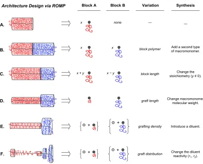
mediated by the fast-initiating G3 catalyst. Macromonomers are stitched together through the backbone, providing access to well-defined bottlebrush polymers. ... 9 Figure 1.5: Opportunities for architectural design via living grafting-through ROMP.
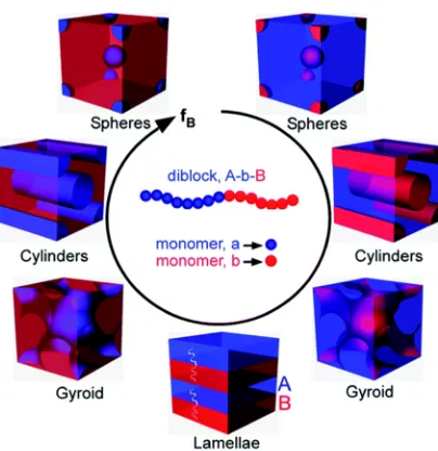
Schematic illustrations of polymer architectures are provided on the left. For ease of visualization, the polymers are illustrated in the limit of fully extended backbones, and cylinders indicate the anticipated local cross-sectional radii of gyration. Red and blue side chains indicate different chemical compositions (i.e., Block A and Block B, respectively). For each row (B–F), the architectural variation compared to the previous row (second to last column) and required synthetic change (last column) are provided. ... 10 Figure 1.6: Equilibrium morphologies observed linear AB diblock polymers, the
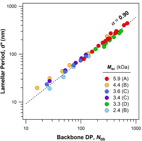
Figure 1.7: Compiled reported examples of the scaling of the lamellar period (d*) with the backbone length (Nbb) for six series of bottlebrush diblock polymers. All polymers are fully grafted and feature symmetric PLA and PS side chains. The average side chain molecular weights (Msc, in kDa) are provided in the legend. The letters in parentheses indicate the corresponding reference: (A) = Ref. 17, (B) = Ref. 94, (C) = Ref. 96, and (D) = Ref. 97. A dotted line corresponding to α = 0.90 is included for comparison. ... 13 Figure 1.8: Self-assembly of (A) linear and (B) bottlebrush diblock polymers to
lamellar morphologies. The scaling of the lamellar period with backbone degree of polymerization (d* ~ Nbbα) differs as a consequence of the
molecular architecture. ... 14 Figure 2.1: Grafting-through ROMP of a small-molecule diluent (white) and a
macromonomer (black). Since the side chains (red) are connected to certain backbone units, control over the backbone sequence directly determines the side chain distribution: (A) uniform, (B) gradient, etc. The anticipated average cross-sectional radius of gyration (Rc) is indicated. For ease of visualization, chains are illustrated in the limit of fully extended backbones. ... 18 Figure 2.2: (left) Structures of macromonomers (PS, PLA, PDMS) and diluents
(DME, DEE, DBE). (right) Plots of ln([M]0/[M]t) versus time, showing first-order kinetics for the homopolymerization of norbornene monomers (0.05 M) catalyzed by G3 (0.5 mM) in CH2Cl2 at 298 K (orange stars: PDMS, inverted red triangles: DME, green squares: PLA, brown diamonds: DEE, purple triangles: DBE, blue circles = PS). The numbers in parentheses indicate kobs (10-3 s-1) under the reaction conditions. ... 20 Figure 2.3: Representative repeated runs to determine khomo (M−1 s−1) for (A) DME
and (B) and PLA. For all diluents and macromonomers studied herein, the measured rate constants are consistent across multiple runs. ... 21 Scheme 2.1: Propagation reactions for the copolymerization of a discrete diluent (M2,
dx-DE shown for example) and a macromonomer (M1) according to a terminal model. M2* and M1* are the corresponding propagating alkylidene species. (A) Diluent self-propagation (k22), (B) propagation (k21), (C) macromonomer self-propagation (k11), (D) cross-propagation (k12). ... 22 Scheme 2.2: Mayo-Lewis terminal model describing the copolymerization of M1 and
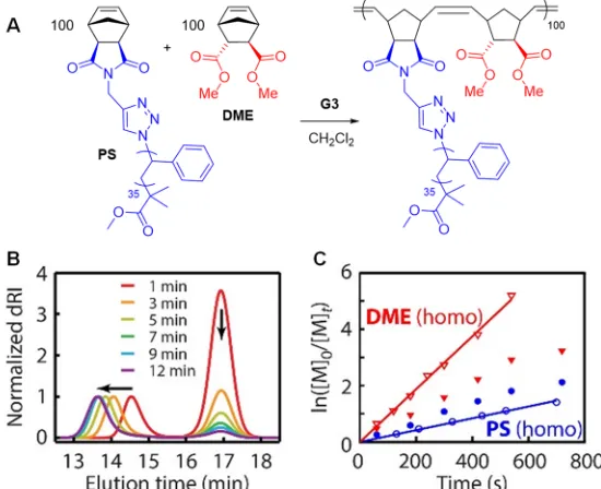
M2. ... 23 Figure 2.4: (A) Copolymerization of PS (0.05 M) and DME (0.05 M) catalyzed by
blue circles = PS, filled red triangles = DME). Unfilled blue circles (PS), unfilled red triangles (DME), and the solid lines, plotted for comparison, were obtained from homopolymerization reactions under the same conditions. ... 25 Figure 2.5: Non-linear least-square curve fitting for the copolymerization of (A, B)
PS (0.05 M) and DME (0.05 M) and (C, D) PS (0.05 M) and DME (0.10 M) in CH2Cl2 at 298 K. [G3]0 = 0.5 mM. Calculated fits (solid lines) show close agreement with the measured values (points). In (B, D), the dashed lines, included for comparison, indicate ideal random copolymerization (r1 = r2 = 1). ... 27 Figure 2.6: Non-linear least-square curve fitting for the copolymerization of various
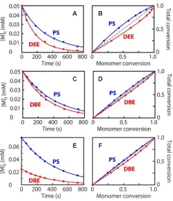
macromonomer/diluent pairs: (A, B) PS (0.05 M) and DEE (0.05 M); (C, D) PS (0.05 M) and DBE (0.05 M); (E, F) PS (0.075 M) and DBE (0.025 M). [G3]0 = 0.5 mM, solvent = CH2Cl2, temperature = 298 K. ... 28 Figure 2.7: Non-linear least-square curve fitting for the copolymerization of various
macromonomer/diluent pairs: (A, B) PLA/DME; (C, D) PLA/DBE; (E, F) PDMS/DME; (G, H) PDMS/DBE (0.055 M). Reaction conditions: [M]0 = 0.05 M unless otherwise indicated, [G3]0 = 0.5 mM, solvent = CH2Cl2, temperature = 298 K. ... 30 Figure 2.8: Simulated copolymer composition for (A) PS:DME = 1:1, (B) PLA:DME
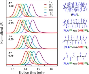
= 1:1, (C) PDMS:DME = 1:1, and (D) PDMS:DBE = 1:1. Insets show schematic illustrations of the corresponding graft polymers; for ease of visualization, the side chains and backbones are shown in the fully extended limit. ... 31 Figure 2.9: SEC traces of (PLAz-ran-DME1-z)n where z = grafting density (1.0, 0.75,
0.50, or 0.25) and n = total backbone degree of polymerization (red: 167, orange: 133, green: 100, blue: 67, purple: 33). ... 32 Figure 2.10: Homopolymerization rate constants (khomo) for substituted
endo,exo-norbornenyl diester monomers (left to right: 1a–j). khomo decreases with increasing steric bulk (R = Me to tBu, 1a–f). khomo does not change significantly with electronic changes via fluorination (1g) or para-substitution of a phenyl ring (1h–j). ... 35 Scheme 2.3: Expanding the scope of monomer design for ring-opening metathesis
copolymerization. ... 33 Figure 2.11: (A) Homopolymerization rate constants (khomo) for monomers with
Figure 2.12: Plot of khomo values for all monomers studied herein. The monomers are sorted according to their anchor groups: left to right: endo,exo-diester (red, 1a–j), endo,endo-diester (yellow, 2a–d), exo,exo-diester (green, 3a–d), endo-imide (blue, 4a–c), and exo-imide (purple, 5a–c and macromonomers). khomo values for methyl-substituted monomers are provided for comparison. ... 37 Figure 2.13: Proposed dissociative ROMP pathway for G3. The DFT-optimized
structures of three catalytically relevant ruthenium catalyst species are shown: (A) six-membered Ru−O chelate, (B) 14-electron vacant species, and (C) olefin adduct. ... 39 Figure 2.14: DFT-calculated free energy diagram corresponding to one ROMP cycle
for endo- (2a, blue) and exo-substiuted (3a, red) norbornenyl monomers. The following intermediates were calculated: (A) six-membered Ru–O chelate, (B) 14-electron vacant species, (C) olefin adduct, and (D) metallacyclobutane. See also Figure 2.13. ... 40 Figure 2.15: (A) Copolymerization scheme: the same macromonomer (PLA, M1) was
copolymerized with 13 different diluents (M2). The feed ratio (x/y = 1) and total backbone length (x + y = 200) were fixed. (B) M2 arranged in order of increasing k22. ... 42 Figure 2.16: SEC traces for PLA + diluent copolymerizations at full conversion. ... 42 Figure 2.17: PLA/diluent copolymerization data. Left axis, black: self-propagation
rate constants (k22: filled circles, k11: open circles). Right axis, red: reactivity ratios (r2: solid line, r1: dotted line) ... 43 Figure 2.18: Simulated sequences and (inset) graft polymer architectures for the
copolymerization of PLA with different diluents: (A) 4a, (B) 1a, or (C) 5a. For ease of visualization, the simulated structures show fully extended side chains and backbones. ... 45 Figure 2.19: Data for the copolymerization of M1 = PDMS (left) or PS (right) with
different diluents. Left axis, black: self-propagation rate constants (k22: filled circles, k11: open circles). Right axis, red: reactivity ratios (r2: solid line, r1: dotted line). ... 46 Figure 2.20: Reactivity ratio map. The copolymerization kinetics studied for PLA,
PDMS, and PS are interpreted in terms of the quotient r1/r2, plotted on the x-axis. For ease of visualization, the simulated structures show fully extended side chains and backbones. ... 47 Scheme 3.1: Illustrations of three AB graft diblock polymers differing only in the side
Figure 3.1: SAXS patterns corresponding to the annealed graft block polymers: (A) BP-1, (B) BP-2, (C) BP-3. The white “x”’ indicates the first-order diffraction peak, q*. ... 61 Figure 3.2: Schematic illustration of the relationships between chain dimensions and
the lamellar period. (A) dA ≈ 3dB is expected if the backbones are fully stretched (since Nbb,A = 3Nbb,B), but it is consistent with SAXS data. (B) Instead, dA ≈ dB is observed. This requires bending of the A block backbone. (C) Illustration of BP-3 and revised chain conformations. ... 61 Figure 3.3: Comparison of simulated (top, middle) and measured (bottom)
1D-averaged SAXS data. The experimental data closely matches the expected SAXS pattern corresponding to lamellae with symmetric (dA = dB) domains. ... 62 Figure 3.4: Self-assembly of linear and bottlebrush diblock polymers into lamellae. ... 63 Scheme 3.2: Synthesis of (PLAz-r-DME1−z)n-b-(PSz-r-DBE1−z)n block polymers
(System I) featuring variable backbone degrees of polymerization (Nbb = 2n = 44–363) and grafting densities (z = 1.00, 0.75, 0.50, 0.35, 0.25, 0.20, 0.15, 0.05, 0). ... 65 Figure 3.5: Scanning electron micrographs of graft block polymers with (A) z =
1.00, (PLA)100-b-(PS)100; (B) z = 0.75, (PLA0.75-r-DME0.25 )110-b-(PS0.75-r-DBE0.25)110; (C) z = 0.50, (PLA0.5-r-DME0.5)104-b-(PS0.5 -r-DBE0.5)104; and (D) z = 0.25, (PLA0.25-r-DME0.75)112-b-(PS0.25 -r-DBE0.75)112. ... 68 Figure 3.6: (top) Scheme of System I, comprising graft block polymers (PLAz
-r-DME1−z)n-b-(PSz-r-DBE1−z)n with variable total backbone degrees of polymerization (Nbb = 2n) and grafting densities (z). (A) Stacked 1D azimuthally averaged SAXS profiles for z = 1, indicating well-ordered lamellar morphologies. (B) Experimental data for the lamellar period (d*) and Nbb (circles), as well as calculated power-law fits (d* ~ Nbbα,
lines). (C) Plot of the scaling exponents (α) as a function of z. A transition occurs around z = 0.2 (dotted line). ... 68 Scheme 3.3: (PLAz-r-DBE1−z)n-b-(PSz-r-DBE1−z)n of variable backbone degrees of
polymerization (Nbb = 2n = 82–533) and grafting densities (z = 0.75, 0.50, 0.35, 0.25, 0.15, 0.12, 0.06, and 0.05). ... 70 Figure 3.7: (top) Scheme of System II, comprising graft block polymers (PLAz
-r-DME1−z)n-b-(PSz-r-DBE1−z)n with variable total backbone degrees of polymerization (Nbb = 2n) and grafting densities (z). (A) Stacked 1D azimuthally averaged SAXS profiles for z = 0.75, indicating well-ordered lamellar morphologies. (B) Experimental data for the lamellar period (d*) and Nbb (circles), as well as calculated power-law fits (d* ~ Nbbα, lines). (C) Plot of the scaling exponents (α) as a function of z. A
unfilled circles correspond to data for System I (z = 1.00), in which the side chain molecular weights are slightly higher. ... 72 Figure 3.8: Plots of predicted Nbb required to access d* = 200 nm as a function of
grafting density (z) for (A) System I and (B) System II. ... 73 Figure 3.9: Analysis of scaling trends with grafting density (z) for (A) System I and
(B) System II. (top) Experimentally determined values and lines of best fit for the scaling exponent (α) versus z. The lines intersect at a critical zc, associated with a transition in the backbone stiffness. In (b), the unfilled circle (z = 1.00) indicates data for System I. (bottom) Calculated root-mean-square end-to-end distances, normalized by the backbone statistical segment length (R2/a0), fixing Nbb = 100. ... 77 Figure 3.10: Reduced zero-shear viscosity (0 / aT) versus Mw for six series with
varying grafting density, z. Unentangled and entangled polymers are shown with open and filled symbols, respectively. Power-law fits are shown corresponding to Rouse (dotted line) or reptation (solid line) scaling. ... 83 Figure 3.11: Dependence of the plateau modulus of graft polymer melts normalized
by the plateau modulus of the analogous linear melt (Ge / Ge,lin) on the average backbone length between grafts (ng). Different conformational regimes are identified as a function of ng at constant Nsc. (A) Regimes predicted by Daniel et al. based on theory.50 Adapted with permission from Nature Publishing Group. (B) Experimental data for (PLAz -r-DME1−z)n graft polymers. ... 84 Figure 3.12: (A) Illustration of a comb polymer at low grafting density, in which the
backbone and side chain are both unperturbed Gaussian coils. The unperturbed backbone length between grafts, Lg,0, and side chain diameter, dsc, are indicated. (B) Entanglement data plotted as Ne,bb / Ne,lin versus dsc / Lg. The black and blue lines correspond to the low- and high-z limits, respectively. When dsc / Lg > 1, steric repulsion between the side chains reduces the density of entanglements. ... 85 Figure 3.13: Direct comparison of the static and dynamic consequences of grafting
density, z. (left axis, red) Scaling exponent α describing the change in the block polymer lamellar period with total backbone degree of polymerization (d* ~ Nbbα). (right axis, blue) Normalized backbone
degree of polymerization between entanglements (Ne,bb / Ne,lin). ... 86 Figure 4.1: Molecular structures and relative interaction parameters for (A) LSO and
(B) LSL' brush triblock polymers. ... 94 Figure 4.2: Schematic of realistic LSO* chain dimensions used in SCFT calculations.
The backbone is treated as a worm-like chain of constant persistence length ξb and fixed contour length L. ... 96 Figure 4.3: (A) TEM of LSO* stained with RuO4. (B) Relative contrast from the
stain, relative widths of corresponding layers observed by TEM, and side chain volume fractions measured by 1H NMR. (C) One LAM3 period with the expected ABCB domain connectivity and layer widths based on data in (B). (D) One LAMP period observed in (A), exhibiting mesoscopic ACBC domain connectivity. ... 97 Figure 4.4: Illustrations and SCFT data distinguishing LAM3 and LAMP
morphologies. In A–D, the light, medium, and dark gray layers represent PLA, PS, and PEO (or mixed PLA/PEO) domains, respectively. (A, B) LSO chain packing in (A) LAM3 and (B) LAMP. (C, D) SCFT composition profiles for LSO* within one normalized lamellar period (z/d0), where (z) is the relative segment concentration of each component. (C) χAC > χC: LAM3 with d* = 43.5 nm. (D) χAC < χC: LAMP with d* = 25.6 nm. (E) SCFT calculations of the normalized free energy (top) and domain spacing (bottom) versus χAC ≡ χLO for LSO*. The transition from mixed (LAMP) to unmixed (LAM3) morphologies is first-order, occurring at a critical value χC (dotted line); for χAB = 0.080 and χBC = 0.049, χC = 0.009. ... 98 Figure 4.5: Lamellar periods (d*) versus normalized molecular weight for brush LSO
(this work) and linear ISO and SIO triblock terpolymers (literature data). Calculated exponents (best fit) to the power law d* ~ Mα are included for comparison. ... 100 Figure 4.6: Consequences of varying end block length NX in LSL' and LSO. (A)
Domain spacing d*. (B) Apparent PLA glass transition temperatures (Tg); for all samples, a single Tg (Tg,PEO < Tg ≤ Tg,PLA) was observed. ... 101 Figure 4.7: Illustration of chain pullout to explain the trends in d* for LSL' and LSO
brush triblock polymers with varying end block length (equivalently, varying molecular asymmetry). Linear chains are depicted to aid visualization. As the end block length NX increases from a fixed parent LS diblock, d* decreases (here, D* ≡ d*/d*LS, where d*LS is the period of the parent LS diblock). (A) X = A' (LSL'): short PLA end blocks pull out of PLA domains into PS domains. (B) X = C (LSO): short PEO end blocks pull out of mixed PLA/PEO domains into PS domains. ... 104 Figure 4.8: (A) Brush LSO triblock terpolymers samples prepared for reflectivity
measurements: NC = 8, 12, 16, 20 (Table 4.1). (B, C) Reference samples, including (B) brush diblock copolymers (SO and LS) and (C) homopolymers of each component (i.e., brush PLA, brush PS, brush PEO, and the polynorbornene backbone). ... 108 Figure 4.9: Representative atomic force micrographs (AFM) corresponding to
dewetted, forming islands and holes. The commensurability conditions differ for brush and linear block polymers. (B) Under optimized conditions, the films wet the substrate. ... 109 Figure 4.10: (A) Experimental (black circles) and simulated (red lines) reflectivity
profiles determined for LSO-12 at three different energies: 286, 284, and 270 eV. (B) Composition profile for LSO-12 determined from reflectivity measurements. The red, green, and blue colors highlight the correspondence between each block and its SLD. ... 110 Figure 4.11: Composition profiles for LSO-12 determined by (A) fitting experimental
reflectivity data or (B) SCFT. The relative segment concentrations of each component are provided over one normalized lamellar period (z / d*). (A) Profiles were determined from RSoXR measurements at 270 eV ( ), 284 eV ( ), and 286 eV ( ); see Figure 4.10. (B) Profiles were calculated for PLA (red), PS (green), and PEO (blue). Comparison of reflectivity and SCFT profiles indicate close agreement between the measured and predicted results. ... 111 Figure 4.12: NEXAFS analysis of LSO-12 at the carbon edge. Arrows indicate
transitions for PS (C=C 1s→π* for the aromatic rings, E = 284.5 eV) and PLA (C=O 1s→π* for the carbonyl, E = 288 eV). ... 112 Figure 4.13: SCFT composition profile for LSO-12 within one normalized lamellar
period (z / d*), where (z) is the relative segment concentration. Calculated profiles for PS (green) and the backbone (black) are shown; PLA and PEO are not included. (See Figure 4.11B.) A schematic illustration of midblock configurations is provided. The arrow indicates a decrease in the backbone concentration at the center of the PS domain, suggesting a large fraction of looping midblocks. ... 113 Figure 4.14: Schematic illustration of chain configurations over one lamellar period
(d*) for LSO-8 (left) and LSO-12 (right). Relevant length scales are indicated, including d*, the thickness of the mixed PLA/PEO layers (dL+O), the thickness of the PS layers (dS), and the average distance between block junctions at the interface (aij). ... 114 Figure 4.15: (A, B) Configurations of looping midblocks inferred from reflectivity
measurements for (A) LSO-8 and (B) LSO-12; see also Figure 4.14. As NC increases from 8 to 12, the thickness of the PS domain (dS) decreases. A concomitant increase in the average distance between block junctions at the interface (aij) is expected. (C) Like SAXS, RSoXR enables determination of d*. However, RSoXR provides additional information due to its sensitivity to chemical composition. ... 116 Figure 5.1: Schematic illustrations of the diverse morphologies identified for linear
Scheme 5.1: Synthesis of LSO brush triblock terpolymers by ring-opening metathesis polymerization (ROMP). The block sequence, backbone lengths, and side chain lengths can be readily varied. ... 123 Figure 5.2: Ternary phase diagram for reported linear ABC triblock terpolymers with
similar frustration (Type II) as LSO. The vertices each represent 100% pure A, B, or C by volume; moving away from a vertex in any direction represents decreasing the volume fraction of the corresponding component. The examples include linear PB-b-PMMA and PS-b-P(E-co-B)-b-PMMA triblocks. ... 124 Figure 5.3: Ternary phase diagram for LSO brush triblock terpolymers. The vertices
each represent 100% pure PLA (L), PS (S), or PEO (O) by volume. Each symbol represents a brush LSO triblock synthesized, annealed, and studied by SAXS. The colors indicate different morphologies: (red) disordered, (green) lamellar, (blue) hexagonally packed cylinders. The shapes indicate different side chain lengths: in the legend on the right, each triplet indicates [ML, MS, and MO], where Mi is the number-average molecular weight (in kg/mol) of each side chain i. Unfilled symbols indicate samples that could not be unambiguously assigned by SAXS. ... 125 Figure 5.4: ABC triblock terpolymers can be classified according to the relative
magnitude of χAC. (A–C) Each circle above represents a block, connected A-B-C from left to right. The contrast between circles represents the relative magnitude of χ; that is, black and white is the highest-contrast pair and therefore represents the highest-χ interaction in the system. (A) If χAC is the smallest interaction parameter, the system experiences Type II frustration. (B) If χAC is larger than one of, but not both, χBC and χAB , the system experiences Type I frustration. (C) If χAC is the largest interaction parameter, the system is non-frustrated. ... 127 Figure 5.5: Ternary phase diagrams for (A) brush SLO and (B) brush LOS triblock
terpolymers. The colors indicate different morphologies: (red) disordered, (green) lamellar, (blue) hexagonally packed cylinders. ... 128 Figure 5.6: SAXS data for an LSO brush triblock terpolymer (NA = 25, NB = 22, NC
= 5) obtained upon heating from 25 to 200 °C at 1 °C/min. The lamellar morphology (LAMP) is stable throughout the entire experimentally accessible temperature range. d* varies slightly (<5%) over this range. No order-disorder transition is observed at any temperature below the onset of decomposition. ... 129 Figure 5.7: Variable-temperature SAXS measurements for (A) 14 and (B)
observed with temperature. (B) When NC is short, features consistent with HEX emerge on heating. ... 130 Figure 5.8: Azimuthally integrated 1D SAXS data for an LSO triblock terpolymer
(NA = 25, NB = 22, NC = 5) annealed in four different ways: (A) Thermally annealed at 140 °C between Kapton under modest applied pressure; (B) thermally annealed at 140 °C in a DSC pan with no applied pressure; (C) dropcast from DCM onto a glass cover slip; and (D) channel-die alignment at 140 °C. SAXS data corresponding to all methods indicate the same morphology (LAM) and period (± 0.5 nm). Note that the discontinuity at q ≈ 0.065 Å-1 in (A) is due to a mask applied when averaging the raw 2D data. ... 131 Figure 5.9: Wide-angle X-ray scattering (WAXS) data for the PEO macromonomer
(MM, i.e., linear PEO), brush PLA-PS parent diblock (LSO-0), and 6 selected LSO-NC triblock terpolymers that self-assemble to LAMP. (These data were obtained at 25°C; variable-temperature WAXS data is provided in Figure C.15.) Reflections at 2θ = 19.1° and 23.2° for LSO-NC (▼, inset) and PEO MM match the (120) and (032) reflections from a monoclinic PEO lattice.46 The parent diblock (LSO-0), which contains no PEO, is amorphous as expected. Crystallization is suppressed in the LSO brush triblock terpolymers compared to neat PEO. (Note: Minor peaks at 31.1° and 36.1° are artifacts present in every sample due to the geometry of the stage.) ... 133 Figure 5.10: Raw 2D SAXS (left, middle) and WAXS (right) data for LSO-NC brush
triblock terpolymers. The same set of samples was measured either (left) 3 days after annealing or (middle, right) 365 days after annealing.. ... 134 Figure 5.11: Changes in d* over one year (2016–2017). d*(2017) / d*(2016) is the
ratio of d* measured by SAXS 365 days after annealing and d* measured 3 days after annealing. When the backbone length of the PEO block is short (NC ≤ 12), no significant change in d* is observed over time. However, when NC is long (NC ≥ 14), d* decreases, concomitant with crystallization of the O blocks observed by WAXS. ... 138 Figure 5.12: Azimuthally averaged 1D WAXS data for LSO-NC, measured 365 days
after annealing. Reflections consistent with PEO crystals are observed for NC ≥ 14 (120 at q = 1.36 Å−1; 132 032 212 112, , , at q = 1.67 Å−1). Traces have been shifted vertically for clarity. ... 139 Figure 5.13: Potential types of confined crystallization in the self-assembly of block
Figure 5.14: (A) Geometry of the wide-angle X-ray scattering stage. The lamellar normalˆnis parallel toˆzand perpendicular to theˆ ˆx y plane. Samples were measured with the X-ray beam along ˆx. (B) Fiber pattern of PEO crystals, constructed by rotating the reciprocal lattice along the c-axis.. ... 141 Figure 5.15: Schematic illustrations of orientations of PEO crystallites with respect to
the lamellar normal, ˆn. The X-ray beam is along ˆx, and the gray planes represent the interface between PLA/PEO and PS domains. (A) Homeotropic alignment: the c-axis of the crystals is parallel to ˆn. (B) Homogeneous alignment: the c-axis is perpendicular to ˆn. (C) Random: no preferred orientation is observed. ... 143 Figure 5.16: Comparison of the (left) 2D WAXS data along ˆx, (middle) PEO crystal
orientation, and (right) inferred brush backbone orientation. (A) NC = 12: homeotropic alignment is observed. c // ˆn suggests that the PEO block backbone is orthogonal to ˆn. (B) NC = 26: homogeneous alignment is observed. c ˆn suggests that the PEO block backbone is parallel to ˆn. (C) NC = 30: random orientations are observed, consistent with the HEX morphology identified by SAXS. ... 145 Figure 6.1: The wavelength of reflection (λ) increases linearly with the lamellar
period (d*), which in turn scales with the total block polymer molecular weight (M). ... 150 Figure 6.2: Predicted lamellar periods (d*) for (A) z = 1.0 and (B) z = 0.5 block
polymers with the same number of side chains (zNbb = 100). Comparing A and B indicates that decreasing z from 1.0 to 0.5 but maintaining the same number of side chains increases d* by 30%. ... 153 Scheme 6.1: Synthesis of block polymers with polyhedral oligomeric silsequioxane
(POSS) and octadecyl (C18) side chains by sequential ROMP. ... 154 Figure 6.3: Scanning electron micrographs of cross-sections of POSS-b-C18 films.
See Table 6.1: (A) Entry 2, (B) Entry 3, and (C) Entry 4. Ruthenium tetroxide (RuO4) was used to preferentially stain POSS domains. ... 155 Figure 6.4: Brush block polymers self-assemble to lamellar arrays with large periods
(d*). Blending with low-molecular-weight linear homopolymers (identical to the side chains of the brush polymer) swells the structures, increasing d*. ... 156 Figure 6.5: (A) Scanning electron micrographs of cross-sections of
corresponds to the ϕHP = 0.45 sample in A–B. Blue: PS brushes and HP; green: PLA brushes and HPr; red: polynorbornene backbone. Solid lines correspond to the brush polymer, and dashed lines correspond to HPs. ... 157 Figure 6.6: Plots of d* versus Nbb for graft block polymers and blends with symmetric
equivalents of linear homopolymers. ϕrel is the relative backbone concentration. A (red circles) represents neat z = 1.00 block polymers (ϕrel = 1.0, A1–A5); B (yellow circles) represents neat z = 0.75 block polymers (ϕrel = 1.3, B1–B4); and C (green circles) represents neat z = 0.50 block polymers (ϕrel = 1.9, C1–C4). B and C were each blended with sufficient amounts of homopolymer to dilute ϕrel to 1.0 (unfilled triangles). Each series was fit to a power law (d* ~ Nbbα), and the scaling
exponents α are provided in the upper right corner. ... 160 Figure 6.7: Plots of d* versus Nbb for graft block polymers and blends with symmetric
equivalents of linear homopolymers. ϕrel is the relative backbone concentration. B (yellow circles) represents neat z = 0.75 block polymers (ϕrel = 1.3, B1–B4); C (green circles) represents neat z = 0.50 block polymers (ϕrel = 1.9, C1–C4); and E (blue circles) represents neat z = 0.25 block polymers (ϕrel = 3.3, E1–E7). C and E were each blended with sufficient amounts of homopolymer to dilute ϕrel to 1.3 (unfilled squares); E was also blended to reach ϕrel = 1.9 (unfilled diamonds). Each series was fit to a power law (d* ~ Nbbα), and the scaling exponents α are provided on the right. ... 161 Figure 6.8: (left) Schematic illustration and (right) chemical structure of
gPS-gPEO-gPS (SOS) brush triblock copolymers... 162 Figure 6.9: Differential scanning calorimetry data for SOS brush triblock copolymers
as functions of LiTFSI loading: (A) gPS11-gPEO78-gPS11 and (B) gPS15-gPEO119-gPS15. Traces are shown for a 5 °C/min ramp rate on heating and are shifted vertically for clarity. ... 164 Figure 6.10: Normalized ionic conductivity (σ/σmax) for gPS11-gPEO7-gPS11/LiTFSI
and gPS15-gPEO119-gPS15/LiTFSI blends, relative to linear PEO (Mn = 300 kDa). ... 166 Figure 6.11: Dynamic mechanical analysis of neat gPS11-gPEO78-gPS11, presenting
the storage (G') and loss (G'') moduli as functions of temperature and frequency (ω). ... 167 Figure 6.12: (A) Brush polymer ion gels were prepared by blending gPS-gPEO-gPS
represent fits to a model using a hard sphere form factor and Percus-Yevick structure factor. Traces are shifted vertically for clarity. ... 169 Figure 6.13: Dynamic mechanical analysis of ϕSOS = 0.16 ion gels containing
gPS15-gPEO119-gPS15 (red) or gPS3-gPEO85-gPS3 (black) at 25 °C, presenting the storage (G') and loss (G'') moduli as functions of frequency (ω). ... 170 Figure 6.14: Ionic conductivities for brush polymer ion gels, normalized to neat
[BMI][TFSI]. Closed and open symbols represent gPS3-gPEO85-gPS3 and gPS15-gPEO119-gPS15 samples, respectively. Polymer concentrations are 9 (□ and ■), 16 ( and ▲), 23 (○ and ●), and 29 wt% (◊ and ♦)... 171 Figure 6.15: Electrocatalytic reduction of CO2 to CO in gPS-gPEO-gPS brush
polymer ion gels. The catalyst, Re(bpy)(CO)3Cl, dissolves in the continuous gPEO / [BMI][TFSI] matrix. ... 172 Figure 6.16: Cyclic voltammetric scans of brush polymer ion gels comprising
gPS15-gPEO119-gPS15, [BMI][TFSI]. (A) Ion gels containing no additives (black); 14.3 mM Fc (green); or 14.3 mM Fc and 15.3 mM CoCp2+ (blue). (B) Ion gels containing 14.3 mM Fc and 1 atm CO2 (black); 5 mM Fc and 10 mM Re(bpy)(CO)3Cl (blue); or 7.1 mM Fc, 14.3 mM Re(bpy)(CO)3Cl, and 1 atm CO2 (green). ... 173 Scheme A.1: Synthesis of cis-5-norbornene-exo-dicarboxylic anhydride (A.1). ...179 Scheme A.2: Synthesis of N-hydroxyethyl-cis-5-norbornene-exo-dicarboximide
initiator (A.2). ...180 Scheme A.3: Synthesis of ω-norbornenyl poly(D,L-lactide) (PLA) macromonomer. ...180 Figure A.1: 1H NMR spectrum of PLA macromonomer in CDCl3...181 Scheme A.4: Synthesis of N-propargyl-cis-5-norbornene-exo-dicarboximide (A.3). ....182 Scheme A.5: Synthesis of PS-Br (A.4) by atom-transfer radical polymerization ...182 Scheme A.6: End group conversion: PS-Br to PS-N3 (A.5) ...183 Scheme A.7: Synthesis of ω-norbornenyl polystyrene macromonomer (PS). ...184 Figure A.2: 1H NMR spectrum of PS macromonomer in CDCl3. ...185 Scheme A.8: Synthesis of N-(hexanoic acid)-cis-5-norbornene-exo-dicarboximide
(A.6). ...185 Scheme A.9: Synthesis of ω-norbornenyl poly(dimethyl siloxane) macromonomer
(PDMS). ...186 Figure A.3: 1H NMR spectrum of PDMS macromonomer in CDCl3. ...186 Scheme A.10: Synthesis of ω-norbornenyl poly(ethylene oxide) macromonomer
Scheme A.12: Synthesis of endo,exo-norbornenyl diester diluents (1e–1j). ...188 Scheme A.13: Synthesis of endo,endo-norbornenyl diester diluents (2a–2d). ...189 Scheme A.14: Synthesis of exo,exo-norbornenyl diester diluents (3a–3d). ...190 Scheme A.15: Synthesis of endo-norbornenyl imide diluents (4a–4c). ...190 Scheme A.16: Synthesis of exo-norbornenyl imide diluents (5a–5c). ...191 Figure A.5: Differential scanning calorimetry (DSC) data for PS100, DBE100, and
two copolymers thereof: (PS100-b-DBE100) and (PS0.5-ran-DBE0.5)200. The data were collected on the second heating cycle using a 10 °C/min ramp rate, and glass transition temperatures (Tg, open circles) were identified from the corresponding derivative curves. Both copolymers exhibit a single Tg between the Tgs of the pure components, indicating successful incorporation of both PS and DBE. The Tg of PS100-b-DBE100 (which has a guaranteed blocky sequence) differs from the Tg of (PS0.5-ran-DBE0.5)200 in terms of both position and shape, suggesting that (PS0.5-ran-DBE0.5)200 is at least not blocky and instead likely random as expected. ...193 Figure A.6: Stacked 1H NMR spectra obtained during the pyridine titration
experiments. To an NMR tube containing a CD2Cl2 solution of the monopyridine complex (11.2 mM) was titrated with a CD2Cl2 solution containing both pyridine (1.47 M) and the monopyridine complex (11.2 mM). The concentration of the monopyridine complex remained constant during the titrations. The chemical shifts of the benzylidene 1H resonance was monitored at 298 K and could be employed to fit the pyridine binding constant (Kbinding = 1/Keq,1). ...195 Figure A.7: ROMP of 5a (left) and 5b (right) in CH2Cl2 at 298 K showing the rate
dependence on [G3]0 (maroon: [G3]0 = 0.5 mM, blue: [G3]0 = 0.05 mM, green: [G3]0 = 0.025 mM). The slope corresponds to the kobs (s -1). These polymerization reactions have the same [5a]0/[G3]0 and [5b]0/[G3]0 ratio of 100. Time-lapse kinetic traces were obtained using our standard homopolymerization procedure...197 Figure A.8: SEC traces for PDMS + diluent copolymerizations at full conversion. ...201 Figure A.9: SEC traces for PS + diluent copolymerizations at full conversion. ...202 Figure B.1: 1H NMR spectra of the co-monomer mixtures for each (PLA0.15
-r-DME0.85)n sample (Table 3.3) prior to initiation. ... 206 Figure B.2: SEC traces for graft block polymers BP-1, BP-2, and BP-3, indicating
essentially identical molecular weights and dispersities. ... 208 Figure B.3: 1H NMR data for graft block polymers BP-1, BP-2, and BP-3, indicating
Figure B.5: Raw 2D SAXS data for z = 0.05 graft polymers: (a) (PLA0.05 -r-DME0.95)200, (b) (PS0.05-r-DBE0.95)200. These polymers correspond to each block of the lowest-grafting-density samples investigated herein. Even at large Nbb, no evidence of microphase separation is observed, suggesting that each block is effectively homogeneous. To a first approximation, χ between the backbone and side chains does not appear significant. ... 214 Figure B.6: Raw 2D SAXS for System II. Compare sample IDs in Table 3.2. ... 215 Figure B.7: SEC traces for (PLAz-r-DME1−z)n graft polymers, where z = (A) 1.00,
(B) 0.50, (C) 0.40, or (D) 0.25. ... 219 Figure B.8: Van Gurp-Palmen plots of the highest-Mw (i.e., most-entangled) sample
for each z. ... 221 Scheme C.1: Synthesis of brush triblock polymers by ring-opening metathesis
polymerization (ROMP): (A) LSO, (B) LSL'. Red, green, and blue structures represent poly(D,L-lactide) (L), polystyrene (S), and poly(ethylene oxide) (O) side chains, respectively. This color scheme is used in all figures. ... 223 Scheme C.2: Synthesis of LSO-NC brush triblock terpolymers with guaranteed fixed
NA and NB. A large batch of the PLA macromonomer (L MM) is polymerized by ROMP to the L brush homopolymer. Addition of the PS macromonomer (S MM) to the same flask obtains a parent LS brush diblock copolymer with controlled NA and NB. The solution of LS is split to 10 vials, and an appropriate volume of a stock solution of PEO macromonomer (O MM) is added to each vial. In this way, 10 different LSO brush triblock terpolymers are obtained, each with the same NA and NB and variable NC. LSL' brush triblock copolymers were synthesized in the same way (replacing O MM with L MM in the last step). ... 224 Figure C.1: Size-exclusion chromatogram (SEC) of LSO* (NA = 28, NB = 27, NC =
5). The peaks are unimodal and narrow, indicating low molar mass dispersity. Complete consumption is observed at each stage prior to addition of subsequent blocks. ... 226 Figure C.2: SEC traces of 10 LSO-NC triblock terpolymers with fixed NA and NB and
variable NC. For these triblocks, NA = 26, NB = 24, and 0 ≤ NC ≤ 20 (Table 4.1). ... 226 Figure C.3: SEC traces of 10 LSL'-NA' triblock copolymers with fixed NA and NB
and variable NA'. For these triblocks, NA = 30, NB = 28, and 0 ≤ NA' ≤ 24 (Table 4.2). ... 227 Figure C.4: (A–C) TEM images of different sections of LSO*. (D)
four-layer lamellar morphology with the same relative domain thicknesses and contrast. Compare Figure 4.3A. ... 230 Figure C.5: Structures and relevant domain spacings indexed by SAXS. Black and
white layers represent two different domains; for simplicity in visualizing the parameters, only two domains are illustrated for lamellae (whereas LAM3 and LAMP each have three domains). The substrate is shown at the bottom of each sample, and the arrow indicates the direction of the X-ray beam. (A) LAM stacked normal to the beam. The relevant spacing is d*, the lamellar period discussed in this report. (B) LAM stacked in-plane with the beam. The relevant spacing is d//. ... 233 Figure C.6: Raw 2D SAXS data for LSO-NC indexed (left) to the P1 space group
along the perpendicular direction, corresponding to lamellae stacked normal to the beam (LAMꞱ) and (right) to the P1 space group along the parallel direction. ... 234 Figure C.7: Azimuthally integrated 1D SAXS patterns for LSO-NC (fixed NA, NB and
variable NC), which obey d* ~ M−0.87. The large change in the position of q* (and therefore d* = 2π/q*) across the series is emphasized by the gray box. All traces correspond to samples that self-assemble to majority LAM. Compare Fig. C.10 (LSL'). ... 237 Figure C.8: TEM images of (A) LSO*, (B) LSO-4, (C) LSO-10, and (D) LSO-14.
All self-assemble to lamellar morphologies, consistent with SAXS. For LSO-NC, the domain spacings were calculated by averaging over 20 periods, and the same trend is observed by TEM and SAXS. As NC increases, d* decreases: d*(LSO-4) = 19.1 nm, d*(LSO-10) = 17.8 nm, d*(LSO-14) = 17.7 nm. The magnitudes of the periods are smaller than those obtained from SAXS, likely due to compression of the sample upon sectioning. The three-phase contrast is clear for LSO* but is challenging to obtain for all images. ... 238 Figure C.9 Raw 2D SAXS data for LSL'-NA' indexed (left) to the P1 space group
along the perpendicular direction, corresponding to lamellae stacked normal to the beam (LAMꞱ) and (right) to the P1 space group along the parallel direction. ... 240 Figure C.10: Azimuthally integrated 1D SAXS patterns for LSL' brush triblock
copolymers with fixed NA and NB and variable NA'. The LSL' series was synthesized from a common parent LS diblock in the same way as LSO with variable NC. The large change in the position of q* (and therefore d* = 2π/q*) across the series is emphasized by the gray box. All traces correspond to samples that self-assemble to majority LAM (i.e., LAM2). Compare Figure C.7 (LSO). ... 243 Figure C.11: DSC data for 10 LSO-NC triblock terpolymers (0 ≤ NC ≤ 20). Traces
pure PLA, PS, and PEO are not observed. Open circles (○) indicate the positions of Tg, determined from the corresponding derivative curves. As NC (and therefore the PEO content) increases, Tg decreases. Compare Fig. C.12 (LSL'). ... 244 Figure C.12: DSC data for 10 LSL'-NA' triblock terpolymers (0 ≤ NA' ≤ 24). Traces
correspond to data collected upon heating from −85 °C to 120 °C at 20 °C/min. We note that under these conditions, the glass transition of PS is not observed. Open circles (○) indicate the positions of Tg, determined from the corresponding derivative curves. As NA' increases, the Tg remains the same (±1 °C). Compare Figure C.11 (LSO). ... 245 Figure C.13: SCFT composition profiles calculated over one lamellar period for two
triblocks that self-assemble to LAMP: (A) LSO-6 and (B) LSO-20. The relative segment concentrations (z) of each component are shown (red: PLA, green: PS, blue: PEO). SCFT predicts a small proportion of PEO blocks mixed in PS domains when NC is small, consistent with the chain pullout model for the unusual d* trend. Profiles were calculated using
χLS = 0.080, χSO = 0.049, χLO = −0.010, and different C block dispersities (Table C.4). ... 246 Figure C.14: SCFT composition profiles calculated over one lamellar period for a
linear LSO triblock terpolymer in which each block has the same molecular weight as the corresponding block in LSO*. The relative segment concentrations (z) of each component are shown (red: PLA, green: PS, blue: PEO). Compare Figure 4.4: both brush and linear LSO triblock terpolymers show a transition from LAM3 to LAMP controlled by the magnitude of χLO. Profiles were calculated using χLS = 0.080, χSO = 0.049, and χLO = 0.034 = χC (the calculated transition between LAM3 and LAMP where each phase is equally stable). (A) For large χLO > χC, SCFT predicts pure domains (LAM3). (B) For small χLO < χC, SCFT predicts LAMP. ... 247 Figure C.15: Variable-temperature WAXS data for (A) PEO macromonomer (MM,



![Figure 2.7: Non-linear least-square curve fitting for the copolymerization of various macromonomer/diluent conditions: [M]pairs: (A, B) PLA/DME; (C, D) PLA/DBE; (E, F) PDMS/DME; (G, H) PDMS/DBE (0.055 M)](https://thumb-us.123doks.com/thumbv2/123dok_us/955206.608713/69.612.199.451.86.470/figure-square-fitting-copolymerization-various-macromonomer-diluent-conditions.webp)