Empirical Data Analytics
Plamen Angelov, Xiaowei Gu, Dmitry Kangin
School of Computing and Communications Lancaster University
Lancaster, LA1 4WA, UK
e-mail: {p.angelov, x.gu3, d.kangin}@lancaster.ac.uk
Abstract:
Finally, a new type of classifier called naïve Typicality-based EDA class is introduced which is based on the newly introduced global typicality. This is only one of the wide range of possible applications of EDA including, but not limited for anomaly detection, clustering, classification, control, prediction, control, rare events analysis, etc. which will be the subject of further research.
Index terms — data mining and analytics, probability, statistics, pattern recognition, machine learning, local and global typicality, eccentricity, centrality.
I.
Introduction
Data analysis can be described as a process which applies statistical and/or formal techniques to describe, illustrate and evaluate data. It became a hot topic recently in many different areas such as biology, econometrics, epidemiology, social science, social media, cyber-security, and so on. Nowadays, new scientific areas are becoming data-centric (if previously data rich were mostly the engineering, natural sciences and, to some extent, economics, now biomedical, social and other sciences are also increasingly becoming data-centric). There is a growing demand for alternative new concepts for data analysis that are centred at the actual data collected from the real world rather than at theoretical prior assumptions which need then to be confronted for verification with the experimental data as is the case with the traditional statistical approach [1]-[4]. The traditional probability theory and statistics assume the actual data to be realizations of imaginary random variables and further assume the prior distributions of these variables.
However, real processes of interest (such as climate, economic, social, mechanical, electronic, biological, etc.) are complex and not always with a clear nature (deterministic or stochastic). A more recent alternative is to approximate the distributions using non-parametric, data-centered functions, such as particle filters [7], entropy-based information-theoretic learning [8], etc. On the other hand, partially trying to address the same problems, in 1965 L. Zadeh introduced fuzzy sets theory [9] which completely departed from objective observations and moved (similarly to the belief-based theory [10] introduced a bit later) to the subjectivist definition of the uncertainty. A later strand of fuzzy set theory (data driven approach) developed mainly in 1990s attempted to define the membership functions based on experimental data which stands in between probabilistic and fuzzy representations [11, 12], however, this approach requires assuming the type of membership function.
Within the Empirical Data Analytics (EDA), we define the main problem as follows: “Given observations of outcomes of real processes/experiments alone, estimate the ensemble properties of the data, such as cumulative
proximity, eccentricity, density and typicality of the data. Furthermore, estimate these for any feasible outcome”.
In this paper, we introduce novel non-parametric estimators of ensemble statistical properties of the data derived entirely from the experimental discrete observations. These include the square centrality, eccentricity (), standardized eccentricity () as well as the local typicality, (). The newly proposed non-parametric
estimators are defined for various distance metrics. Furthermore, in this paper we introduce the global typicality
(τG) which is similar (but different) to the histograms. The typicality looks very similar to the well-known pdf, it sums up to 1 and is always positive; however, it is discrete and is always less than 1 while the pdf can paradoxically be greater than 1. Additionally, the typicality is only defined for feasible values of the independent variable while pdf can, paradoxically, be positive even for infeasible values, e.g. negative height, distance, weight, absolute temperature, etc.
The remainder of the paper is organized as follows. In section II, we introduce the basic elements of the Empirical Data Analysis (EDA). The concepts of the local and global typicality as well as estimation for hypothetical new points are described in section III. The properties of the EDA quantities are discussed in section IV. In section V an example of the newly proposed naïve EDA classifier is described and, finally, section VI concludes the paper outlining the future development.
II.
Basic Elements of the Empirical Data Analysis
a) cumulative proximity, q and its inverse, called square centrality, S; b) eccentricity, ξ and standardised eccentricity, ε;
c) density, D;
d) local and global typicality, τ, τG.
The global typicality, τG addresses the global properties of the data and will be introduced in the next section.
First, let us define the data space, M with a distance d
, . Let us consider a finite multiset of data points
1, 2,...,
, , 1 ,k k i k i k
x x x x where the index k denotes the amount of data samples/points/vectors.
p is the dimensionality of the data.
A. Centrality
First, we will recall from the graph and network theory the so called measure of centrality, C [13,14]. Indeed, for every point xikone may need to quantify how close or similar this point is to all other data points from k. In graph (networks) theory a measure of centrality[13] is defined as the inverse of the so called farness which itself is a sum of distances from a point to all other points:
1
1 1
1
( ) , ; 1; ; 1 ;
,
k
k i k i j i k j j i
j i j j
C d k i k
d
x x x x x x x
x x
(1)
Notice that in this and further notations, k denotes the amount of data samples at the moment of the analysis. For the offline cases this is usually denoted by N to represent the total amount of data available and is not changing throughout the analysis while in online cases the data is a stream rather than a set and k may or may be associated with the order of data samples which usually but nt necessarily always is the time instant.
B. Cumulative proximity
In our earlier works [15-16] we defined a measure called cumulative proximity, qk
xi xikwhich can be seen as a square form of the farness, as follows:
2
1, ; 1;
k
k i i k
j
q d k
The cumulative proximity, plays an important role in the definition of the other association measure derived empirically from the observed data without making any prior assumptions about their generation model, namely the typicality and eccentricity as we will see later.
C. Square centrality
It is convenient to consider the square centrality defined as inverse of the cumulative proximity:
1 1
; 1
k
k i i k
k i
S q k
q
x x
x (3)
D. Eccentricity
The eccentricity, k
x is defined within EDA as a normalized cumulative proximity [15,16]. It is a very important measure of the ensemble property related to the tail of the distribution and is empirically derived from the observed data only without making any prior assumptions about their generation model. It plays an important role in anomaly detection [16], analysis of rare events as well as for the estimation of the typicality as it will be detailed further. The eccentricity of a particular data sample xi(xik) is calculated as follows:
1 2; ; 1;
k i
k i k i k k
k j j q k q
x x x x (4)where, the coefficient 2 is included to compensate distance duplication in the denominator which, at the same time, leads to the following bounds for the eccentricity value:
0 xi 1; xik; k k 1 (5)
The denominator must not be zero; from the metric definition it follows that at least two points within the dataset k need to be distinctive. Another property of the eccentricity is that it sums over to 2:
12; ; 1
k
i i k k
i
k
x x (6)
12
; ; 1
1
k i
k i k i k i k k
k j j
q
k k
q k
x
x x x
x
(7)
Standardised eccentricity is more convenient to use in the well-known Chebyshev inequality which within TEDA has a more elegant form.
Fig.1 Standardized eccentricity, ε for real climate data (temperature and wind speed) measured in Manchester, UK for the period 2010-2015 [19].The data with higher standardized eccentricity, are marked with red ellipsoids; these are days with stronger wind (stormy days). As it will be described in the next subsection, values of ε between 5 and 10 correspond to so called
2 ; 3
interval from the mean. [image:6.595.207.397.198.346.2]E. Density
[image:6.595.200.396.517.667.2]The density within the data space plays an important role in data analysis [15-17]. Within EDA it can be defined as the inverse of the standardised eccentricity:
1( ); ; 1k i k i i k k
D x
x x k (8)F. Chebyshev inequality
The Chebyshev inequality [18] is well known in the traditional probability theory and statistics. It describes the probability that certain data sample, x is more than n distance away from the mean where denotes the standard deviation [1-3] and can be formulated as follows [18] if use Euclidean type of distance:
2 2 2
2 1
1 ; ; 1
k i k i k k
P n k
n
x x
(9)
Respectively, the probability the point xi to be an outlier is given by:
2 2 2
2 1
; ; 1
k i k i k k
P n k
n
x x
(10)
It can be proven that exactly the same result can be provided within EDA through the standardized eccentricity [16] for the Euclidean distance:
2
2 1
( ) 1 1 ; ; 1
k i i k k
P n k
n
x x (11)
and, respectively,
2
2 1
( ) 1 ; ; 1
k i i k k
P n k
n
x x (12)
Similarly, the Chebyshev inequality in the form of density are as follows.
2 2
1 1
( ) 1 ; ; 1
1
k i i k k
P D k
n n
x x (13)
2 2
1 1
( ) ; ; 1
1
k i i k k
P D k
n n
x x (14)
G. Recursive calculations
One important aspect of the proposed EDA approach is that the operators defined within it can be calculated recursively for various Hilbert space metrics, e.g. Euclidean, Mahalanobis, even value Minkowski as well as for cosine similarity, which makes EDA suitable for live data streams processing. Consider the time instance the data point xk arrives, it is easy to see that:
2
1 , ; 1; ; 1 1
k i k i i k i k
q x q x d x x k x i k (15)
and respectively
11 2
1 , ; 1; ; 1 1
k i k i i k i k
S x S x d x x k x i k (16)
1) Euclidean type metric
For example, for the Euclidean type distances we have [15-17]:
T T
T 2
; 1; ; 1
k i i k i k k k k
i k i k k i k
q k X
k k i k
x x x
x x x
(17)
where k2 Xk kT k. And, respectively:
T T 1 T T 1 1; 1; ; 1
k i
i k i k k k k
i k i k k k k i k
S x
k X
X k i k
k x x
x x x
(18)
1 1 1
1 1
;
k k k
k
k k
x x
(19)
T T
1 1 1 1
1 1
;
k k k k
k
X X X
k k
x x x x (20)
The total square centrality of the whole dataset and the total cumulative proximity, respectively, can also be updated recursively for each new data point, xk:
1
T
1 1 1
1 1
2 2 ; 0
k k
k i k i k k k k k
i i
q q q k X q
x
x x
x (21)2) Mahalanobis distance
For the case of Mahalanobis type distance recursive update is also possible [15-17]:
T 1
T 1
k i i k k i k k k k k
q x k x
x
X
(22)and, respectively:
T
11 T 1
1
k i i k k i k k k k k
S X
k
x x x (23)
where the covariance matrix k is defined as follows:
T1
1 1
k
k i k i k
i
k
x x (24)
which itself can be updated recursively [1]-[3]. However, the average scalar product Xkis defined differently
from the case when Euclidean distance is used, namely, T 1 1
1 k
k i k i
i
X x x
k
. Thanks to the covariance matrixsymmetricity [20], there is:
1
2 T 1 2
1 1 1
1 1
2 2 2 ; 0
k k
k i k i k k k k k k
i i
q q q k X k p q
x
x x μ Σ μ x (25)III. Typicality and Estimation for Hypothetical Data Points
A. Local typicality
In EDA we define the localtypicality, of a data pointas normalized square centrality or, which is the same, normalized inverse cumulative proximity:
1; ; 1
k i
k i k i k k
(a) Local typicality, (b) pdf
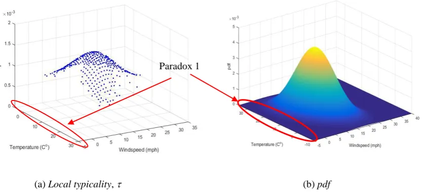
Fig. 3 A comparison of the local typicality distribution, (x) and the traditional pdf based on the same real climate data [19] as in Fig. 1 and 2. The red oval indicates infeasible values of negative wind speed which have pdf>0 according to the pdf. τ is only defined for feasible values (in this case only for positive values of the wind speed).
It is very interesting to stress that the local typicality resembles the well-known pdf, but is free from paradoxes that can be the case with the pdf. Figure 3 visualizes for the same real data [19] the paradox 1 that a Gaussian type pdf may have non-zero values for infeasible values (e.g. negative wind speed).
Fig. 4 further demonstrates another paradox (paradox 2) that pdf values can be >1.
[image:10.595.81.503.496.692.2](a) Local typicality, (b) pdf
Fig. 4 Examples of the paradox 2 regarding the temperature and wind speed. The red ellipsoid indicates the area exhibiting infeasible values of pdf that pdf >1.
Paradox 1
B. Global typicality
It is well known that the traditional pdf expressed as Gaussian or Cauchy function are not perfect to cover real distributions. It is also a well-known technique to use mixtures of distributions [21]. Within EDA it is possible to use a mixture of local typicality distributions derived after clustering the data [22], however, it is also possible to derive a global typicality, G from data directly without clustering or any other pre-processing or prior assumptions. In this paper we define the global typicality, G as a weighted normalised square centrality where the weights are the frequency of occurence of a particular data sample, f.
Let us first introduce couple of definitions. For each dataset k, one can construct a corresponding unique data points set as Uk
u u1, 2,...,ui,...,ul
(uik; where l is the number of the unique data samples) and thecorresponding numbers of times of occurrence by Fk
f1,f2,...,fi,...,fl
. We can also view fi as a frequencyand optionally divide by k. if we prefer values that are 1 . Then the global typicality, G can be defined within EDA on the domain of Uk as follows:
1
1
; 0; 1; 1
u l
i k i
G u
k i l j k j
u j
j k j j
f S
f S l i l
f S
u
u u
u
(27)
where Sku
ui 0 denotes the square centrality at a particular unique data sample ui to all other unique data samples of the data space.Some illustrative examples of applying the global typicality are provided further. It is interesting to note that for small values of k, the global typicality is exactly the same as the frequentistic form of probability (see Fig. 3 and 4), and with large k, the local typicality approximates the well-known Gaussian and Cauchy type pdf.
Let us start with a trivial primer and consider a small data set
2;6; 2; 2;6
. It is also straightforward todetermine U5
2;6 ;l2; k5;lk ; F5
3; 2 . Let us consider Euclidean type distance. The globaltypicality is easy to calculate for this case using equation (3) for S
1/16;1/16
and equation (27) for Gbuttaken only in regards to the unique data, U instead of all data, . The final result,
G
x2
3 / 50.6 and
6
2 / 5 0.4G x
is exactly the same as the frequentistic probability expressed as a ratio of specificFig. 5 Global typicality, τG directly calculated from the data for the trivial primer
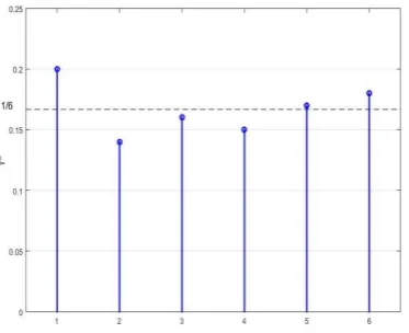
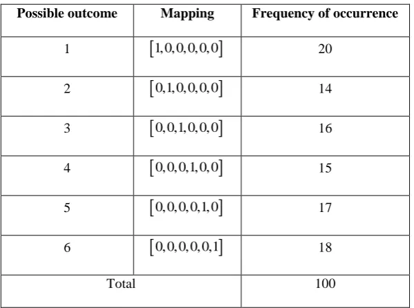
Another example where the global typicality has exactly the same values as the frequentistic probability is if consider fair games which are clearly random. It has to be stressed that the encoding of the values is important. For example, if consider tossing a coin it is easy to encode the two possible outcomes by any number, but if consider a dice which has 6 possible outcomes these usually have an integer number of dots on them (1,2,3,4,5, and 6). Because within EDA the distance between different outcomes is also taken into account as well as the frequency, f the possible outcomes have to be first encoded in such a way that the distance between each pair of outcomes is exactly the same. For example, for 1 we can use
1;0;0;0;0;0
, for 2 we can use
0;1;0;0;0;0
, etc. Then if we have throwing a dice 100 times (or 100 people throwing a dice once) the possible outcomes may be as tabulated in Table 1. It is easy to check that S
0.1;0.1;0.1;0.1;0.1;0.1
and F
17;14;15;15; 21;18
. [image:12.595.213.400.520.672.2]Table 1. Throwing dices (a fair game, random data)
Possible outcome Mapping Frequency of occurrence
1
1,0,0,0,0,0
202
0,1,0,0,0,0
143
0,0,1,0,0,0
164
0,0,0,1,0,0
155
0,0,0,0,1,0
176
0,0,0,0,0,1
18Total 100
The global typicality of each possible outcome is depicted in Fig. 6. It is easy to see that the values of τG fluctuate around the value of 1/6 and they would have all have value of 1/6 if the frequencies of occurrence of each value were the same. The more times we throw the dice, the closer the values of the τG will be to the value of 1/6 exactly the same as the frequentistic probability. In this case, obviously the traditional pdf [1-4] will be misleading although paradoxically the infamous iid conditions are satisfied.
same effect if it is far from the mean (e.g. temperature 26oC) or close to the mean (e.g. 14oC). In the case of a traditional histogram the effect of adding multiple new samples will be the same regardless of the position. Moreover, the global typicality is describes by a closed analytical form equation (27).
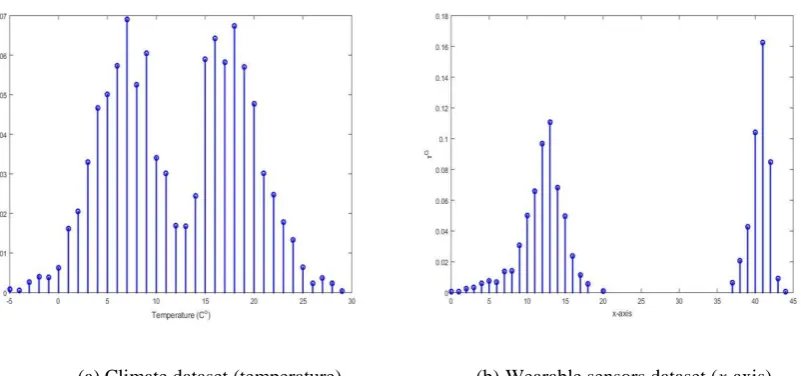
[image:14.595.95.496.151.339.2](a) Climate dataset (temperature) (b) Wearable sensors dataset (x-axis)
Fig. 7 2Dglobal typicality, τG (left plot: temperature [19]; right plot: horizontal acceleration for the wearable devices data [23]).
Notice that the modes (2 on the left plot of Fig. 7 and 5 on the right plot) appear automatically and are not pre-defined). 3D examples (τG vs 2 variables) for the same data are depicted in Fig. 8.
(a) Climate dataset [19] (b) Wearable sensors dataset [23]
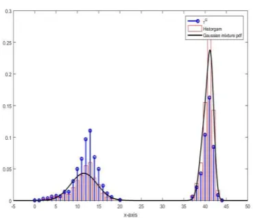
[image:14.595.81.502.477.643.2](a) Gaussian mixture pdf (b) Histogram
Fig. 9 An visual comparison for the same real dataset [19] as the one used in Fig. 1-4, 7a and 8a. (The left hand plot depicts the Gaussian mixture pdf derived by clustering; the right plot – the histogram)
C. Estimating the global typicality of hypothetical points
The mechanism described so far does represent the globaltypicality of data that have been facts (took place and is available). Often of interest is to estimate the global typicality (similar to the probability, likelihood) of hypothetical data points, xk1. The approach we take within EDA is to consider such points (even if they are multiple) one by one to avoid accumulation of errors. In general, there are two options:
i) either the new datum xk1belongs to the corresponding unique values set Ul and one can just increment the number of occurrence within Fl, or
ii) the datum does not belong to Ul. In the latter case, one should append the unique data samples set from Ul
u u1, 2ul
to Ul1
u u1, 2,,u ul, l1
, ul1xk1.After that, for Euclidean and Mahalanobis distances, one needs to update the mean value and the (co-)variance taking into account this new datum. For example, for the Euclidean case, we can recursive calculate the squared centrality of the new data point/sample asul1 given Ul1 l 1:
1 1 1 1
1 ;
1 1
l l l
l
l l
u u
(28)
T T
1 1 1 1 1 1 1
1
;
1 1
l l l l
l
U U U
l l
where l denotes the mean value for the l unique locations in the data space;
l
U denotes the scalar product of the l unique locations in the data space.
T
1T
1 1 1 1 1
1 1 1
1 1
l l
u
k l l l l l l
S U l
u u u (30)
Further, we estimate the frequency of the hypothetical data sample based on the frequencies of the nearest actual data samples. If the hypothetical data point is surrounded by actual data points from both sides per dimension (interpolation case) then we estimate the frequency as the average of the frequencies of the neighbouring data points:
1, , , , 1, ,
1
1 , ,
1 p i L i R i R i l i L i
l
i R i
l
L i
u u f u u f
f
p u u
(31)where uR i, and uL i, are the ithdimensional values of two existing unique locations that are the nearest to ul1 in the ith dimension and satisfy uL i, ul1,iuR i, .
In case, if the estimation is for a hypothetical data point that is outside of the range of the actual data (extrapolation) the frequency is set to 1:
1 1 l
f (32)
Finally, the global typicality is estimated using (27) in regards to ul1:
1 1 1 1 u l k l Gk l l
u j k j j f S f S
u u u (33)To illustrate the estimation of the globaltypicality of hypothetical new data points, let us start again with a trivial primer and work it out step by step. Let us consider a trivial dataset that consists of a single variable, x with 2 experimentally observed values: x12 andx26. It is easy to find that:
k
1, 2 ; d12d214; p1p216; S1S21/16; f1 f21; t1 t2 1/ 2Fig. 10 Illustrative example of estimation of the global typicality for hypothetical data points (in red and green); a comparison with the traditional Gaussian pdf for our trivial primer.
[image:17.595.218.399.77.233.2](a) Climate dataset (Temperature) (b) Wearable sensors dataset (x-axis)
[image:17.595.94.497.315.498.2](a) Climate dataset (b) Wearable sensors dataset
Fig. 12 3D-examples of estimation of the global typicality for real climate dataset [19] and the wearable sensors dataset [23] (blue points –real data; red – estimations at hypothetical points)
(a) Climate dataset (temperature) [19] (b) Wearable sensors dataset (x-axis) [23]
[image:18.595.91.501.79.264.2]Fig.13 Examples of 2D global typicality graphs (blue points –real data; red – estimations at hypothetical points)
Quite logical and trivial, but, importantly, we did not make any assumption about the amount of data, their (in)dependence and generation model. We only selected the distance metric (in this case, Euclidean). Moreover, in this case (because the amount of data is small and does not require recursive calculations) we did not even calculate the mean and standard deviation. The traditional approach will require a number of assumptions to be made and the pdf that can still be build will have non-zero values for many different values of the variable, x for which we do not know where the feasibility region is. If apply the proposed in this paper EDA approach, we will not make these paradoxical conclusions/generalisations, but will be firmly based on the observed experimental data plus the feasible hypothetical values of the variable, x at which we may decide to estimate the global typicality or other ensemble data properties as per EDA. It is also obvious that the results if use EDA will be identical to the well-known frequentistic probability [1-4], see Fig. 10.
Some more interesting examples of estimation of the global typicality based on the climate [19] and wearable sensors datasets [23] that were considered earlier are shown in Fig. 11 (2D) and Fig. 12 (3D).
It has to be stressed that the estimation is made for one hypothetical data point at a time to avoid accumulation of errors. However, if we repeat estimation many times (estimating the value of the global typicality for many hypothetical data points) we can get a globaltypicality graph that looks like continuous (it is not continuous because the total number of data points both existing and hypothetical is countable), see Fig.13.
IV. Properties of the EDA Operators
The typicality resembles the well-known traditional pdf and histograms and has itself the following additional properties:
a) it sums up to 1;
b) its value is within the range
0;1 ;c) is provided in a closed analytical form, equation (27).
data distribution that results in inappropriate estimation. Besides, in order to use Gaussian mixture model, one needs to select somehow the number of components (fixed number of components as in ARD-EM [24], or nonparametric methods [25]); however, this problem does not exist in the proposed approach.
One interesting property of the density, D is that for the case when Euclidean type of distance is used it takes a form of the well-known Cauchy type pdf , except for the fact that normalisation is needed to ensure integration to 1 [1-3]:
T
21
; ; 1
1
k i i k k
i k i k
k D k x x
x x
(34)
That is, for the case of Euclidean type distance:
21 12
1 2
( ) ( ) ; ; 1
p C
k i p k i i k k
p k p
pdf D k
x x x (35)
where is the well-known constant,
is the gamma function.Furthermore, if Mahalanobis type of distance is used it is also of Cauchy type, and a normalisation operation is needed to turn it into the well-known Cauchy type pdf:
T 1 1
1
; ; 1
1
k i i k k
i k k i k
D k p x x
x
x
(36) That is,
1 2 1 2 2 2 1 2( ) ; ; 1
1
det 2
p C
k i p p k i i k k
k p
pdf D k
p
x x x
(a) Climate dataset (temperature) [19] (b) Wearable sensors dataset (x-axis) [23]
(c) Wearable sensors dataset (y-axis) [23] (d) Wearable sensors dataset (z-axis) [23]
Fig. 14 The comparison between histogram, Gaussian mixture pdf and global typicality for the same real climate dataset [19] and the wearable sensors dataset [23] (2D plots).
Furthermore, and interesting property of the standardised eccentricity if one use Euclidean type distance is that the well-known pdf can be defined through the standardised eccentricity as follows:
2 2
( ) 2 2 1
( ) ; ; 1
2
k k i k
G
k i i k k
k
pdf e k
x
x x (38)
Indeed, it can be shown that:
T
2 ; ; 1
k k i i k i k i k k k
[image:21.595.311.496.76.235.2]V. Naïve Typicality-based EDA Classifier
Naïve Bayes classifiers are well known [1]-[3]. They perform classification based on the dominant per class likelihood expressed by a pre-defined (usually, Gaussian) pdf. In this paper, we borrow this concept and introduce naïve Typicality based EDA classifier (T-EDA) built on the basis of data distribution with their global typicality instead of a pre-defined smooth (but idealized) pdf.
Assuming we have C classes at time instance k and let us have the global typicality per class, Gk j, (
1, 2, ,
j C), for data samplexk1, its label is given according to the following equation:
1
,
1
1arg max C
G
k k j k
j
label
x x (40)
Here, the global typicality of the vthclass is calculated by the following equation:
, 1 , 1
, 1
, , ,
1 1
v j
u v l k v k G
k v k l C
u j i k j j i j i
f S
f S
x x
u
(41)
where the index lv indicates the number of unique points in the vth class;
1, 1 , 1
u u
k v k k v k
S x x and , 1
v v l
f are calculated per class.
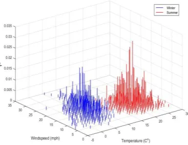
Fig. 15 3D plot of the global typicality (wind speed, temperature and the value of G) for the same data with the two classes (winter and summer) shown with different colour.
[image:22.595.209.402.497.646.2]The performance of the proposed naïve T-EDA classifier is further tested on a well-known challenging problem called PIMA dataset [26]. The performance of the proposed naïve T-EDA classifier was compared against the naïve Bayes, SVM[27] , eClass0[28] and Simpl_eClass0[29]classifiers. First, 90% (691 points) of the data set were used for training. In this paper we use the following attributes:
[image:23.595.94.498.176.373.2](a) Temperature (b) Windspeed
Fig. 16 A 2D plot of τ vs the variable (temperature or the wind speed) for the same climate data [19]. The two classes (winter and summer) are shown with different colour. Left plot, (a): temperature, and right plot, (b): wind speed.
1) number of times pregnant;
2) plasma glucose concentration a 2 hours in an oral glucose tolerance test (mg/dl);
3) diastolic blood pressure (mm Hg);
4) triceps skin fold thickness (mm);
5) body mass index (weight in kg/(height in m)2);
6) diabetes pedigree function.
Table 2 Confusion Matrix for the Validation Data
Methods Actual\Classification Negative Positive
Fig. 17 Overall performances of the five classification approaches
VI. Conclusion and Future Direction
In this paper, we propose an approach to data analysis which is based entirely on the empirical observations of discrete data samples and the relative proximity of these points in the data space. At the core of the proposed new approach is the typicality - an empirically derived quantity which resembles probability. This non-parametric measure is a normalised form of the square centrality. It is also closely linked to the cumulative proximity and eccentricity. In this paper, we introduce and study two types of typicality, namely local and global versions. The local typicality resembles the well-known pdf, probability mass function and fuzzy set membership but differs from all of them. The global typicality, one the other hand, resembles well-known histograms but also differs from them. A distinctive feature of the proposed new approach, EDA is that it is not limited by restrictive impractical prior assumptions about the data generation model as the traditional probability theory and statistical learning approaches are. Moreover, it does not require an explicit and binary assumption of randomness or determinism of the empirically observed data, their independence or even their number which can be as low as couple of data samples. The typicality is considered as a fundamental quantity in the pattern analysis and is derived from the data directly and in a discrete form in a contrast to the traditional approach where a continuous pdf is assumed a priori and estimated from data afterwards. The typicality introduced in this paper is free from the paradoxes of the pdf. Typicality is objectivist while the fuzzy sets and the belief-based branch of the probability theory are subjectivist. The local typicality is expressed in a closed analytical form and can be calculated recursively; thus, computationally very efficiently. The other non-parametric ensemble properties of the data introduced and studied in this paper, namely, the square centrality, cumulative proximity and eccentricity can also be updated recursively for various types of distance metrics. Indeed, different metrics can be used, not only the usually used ones.
In short, the EDA operators as introduced in this paper, have the following properties:
They are entirely based on the empirically observed experimental data and their mutual distribution in the data space;
They do not require any user- or problem-specific thresholds and parameters to be pre-specified;
The individual data samples (observations) do not need to be independent or identically distributed; on the contrary, their mutual dependence is taken into account directly through the mutual distance between the data points/samples;
They also does not require infinite number of observations and can work with as little as 2 data samples;
They are free from some well-known paradoxes of the traditional probability theory;
They can be calculated recursively for many types of distance metrics;
In addition, a new type of classifier called naïve Typicality-based EDA class is introduced which is based on the newly introduced global typicality. This is only one of the wide range of possible applications of EDA including, but not limited for anomaly detection, clustering, classification, control, prediction, control, rare events analysis, etc. which will be the subject of further research.
Acknowledgements
This work was supported partially byThe Royal Society grant IE141329/2014 “Novel Machine Learning Paradigms to address Big Data Streams”.
References
[1]
T. Hastie, R. Tibshirani, J. Friedman, The Elements of Statistical Learning: Data Mining, Inference, and Prediction, 2nd Edition, Springer, 2009, ISBN-13: 978-0387952840.[2]
C. Bishop, Pattern Recognition and Machine Learning, Springer, 2007, ISBN-13: 978-0387310732.[3]
R.O. Duda, P.E. Hart, and D.G. Stork. Pattern Classification – 2nd Ed., Wiley-Interscience, Chichester, West Sussex, UK, 2000.[4]
T. Bayes, An Essay Towards Solving a Problem in the Doctrine of Chances, Philosophical Transactions of the Royal Society, London, England, v.53, p.370, 1763.[5]
A. N. Kolmogorov, Teoriya Veroyatnostey (Probability Theory) in Russian; published in English in 1963, American Mathematical Society, Providence, RI and republished in three volumes by the MIT Press, Cambridge, MA, reprinted 1999.[7]
P. Del Moral, Non Linear Filtering: Interacting Particle Solution, Markov Processes and Related Fields, vol. 2 (4), pp. 555–580, 1996.[8]
J. Principe, Information Theoretic Learning: Renyi's Entropy and Kernel Perspectives, Springer, 2010, ISBN: 978-1-4419-1569-6.[9]
L. A. Zadeh, Fuzzy sets, Information and Control, v. 8 (3): 338–353, 1965.[10]
G. Shafer, A Mathematical Theory of Evidence, Princeton University Press, 1976, ISBN 0-608-02508-9.[11]
M.-Y. Chen, D. A. Linkens, "Rule-base self-generation and simplification for data driven fuzzy models."Fuzzy Systems. The 10th IEEE International Conference on. Vol. 1. IEEE, 2001.
![Fig. 2 The density for the same real climate data as shown in Figure 1 [19]. The data with lower density D are](https://thumb-us.123doks.com/thumbv2/123dok_us/9358926.438046/6.595.207.397.198.346/fig-density-real-climate-shown-figure-lower-density.webp)
![Fig. 9 An visual comparison for the same real dataset [19] as the one used in Fig. 1-4, 7a and 8a](https://thumb-us.123doks.com/thumbv2/123dok_us/9358926.438046/15.595.88.501.81.270/fig-visual-comparison-real-dataset-used-fig-a.webp)
![Fig.11 Examples of estimation (interpolations and extrapolation) of global typicality for the climate [19] and](https://thumb-us.123doks.com/thumbv2/123dok_us/9358926.438046/17.595.218.399.77.233/fig-examples-estimation-interpolations-extrapolation-global-typicality-climate.webp)
![Fig. 12 3D-examples of estimation of the global typicality for real climate dataset [19] and the wearable](https://thumb-us.123doks.com/thumbv2/123dok_us/9358926.438046/18.595.91.501.79.264/fig-examples-estimation-global-typicality-climate-dataset-wearable.webp)