warwick.ac.uk/lib-publications
Original citation:
Dinh, Quang Truong, Marco, James, Yoon, J. I. and Ahn, K. K. (2018) Robust predictive
tracking control for a class of nonlinear systems. Mechatronics, 52. pp.
135-149. doi:10.1016/j.mechatronics.2018.04.010
Permanent WRAP URL:
http://wrap.warwick.ac.uk/102758
Copyright and reuse:
The Warwick Research Archive Portal (WRAP) makes this work by researchers of the University of Warwick available open access under the following conditions. Copyright © and all moral rights to the version of the paper presented here belong to the individual author(s) and/or other copyright owners. To the extent reasonable and practicable the material made available in WRAP has been checked for eligibility before being made available.
Copies of full items can be used for personal research or study, educational, or not-for-profit purposes without prior permission or charge. Provided that the authors, title and full bibliographic details are credited, a hyperlink and/or URL is given for the original metadata page and the content is not changed in any way.
Publisher’s statement:
© 2018, Elsevier. Licensed under the Creative Commons Attribution-NonCommercial-NoDerivatives 4.0 International http://creativecommons.org/licenses/by-nc-nd/4.0/
A note on versions:
The version presented here may differ from the published version or, version of record, if you wish to cite this item you are advised to consult the publisher’s version. Please see the ‘permanent WRAP URL’ above for details on accessing the published version and note that access may require a subscription.
1
Robust Predictive Tracking Control for
A Class of Nonlinear Systems
T.Q. Dinh1,*, J. Marco1, J.I. Yoon2, K.K. Ahn3
1 Warwick Manufacturing Group (WMG), University of Warwick, Coventry CV4 7AL, UK; 2 Korea Construction Equipment Technology Institute, Jeollabuk-do Gunsan 573-540 Sandan-ro 36, Korea;
3 School of Mechanical Engineering, University of Ulsan, Namgu Muger2dong, Ulsan 680-749, Korea;
* Correspondence: [email protected]; Tel.: +44-2476-574902
ABSTRACT
A robust predictive tracking control (RPTC) approach is developed in this paper to deal with a class of nonlinear SISO systems. To improve the control performance, the RPTC architecture mainly consists of a robust fuzzy PID (RFPID) –based control module and a robust PI grey model (RPIGM) –based prediction module. The RFPID functions as the main control unit to drive the system to desired goals. The control gains are online optimized by neural network-based fuzzy tuners. Meanwhile using grey and neural network theories, the RPIGM is designed with two tasks: to forecast the future system output which is fed to the RFPID to optimize the controller parameters ahead of time; and to estimate the impacts of noises and disturbances on the system performance in order to create properly a compensating control signal. Furthermore, a fuzzy grey cognitive map (FGCM) –based decision tool is built to regulate the RPIGM prediction step size to maximize the control efforts. Convergences of both the predictor and controller are theoretically guaranteed by Lyapunov stability conditions. The effectiveness of the proposed RPTC approach has been proved through real-time experiments on a nonlinear SISO system.
Keywords
2
1.
Introduction
Nowadays, automation in control has been applied more and more in the modern life. However, most of industrial machines are nonlinear systems with large uncertainties which cause challenges to design the controllers. Conventional PID controllers are commonly used in industry due to their simplicity, clear functionality and ease of implementation. However, this type of controllers may not perform well for nonlinear, complex and vague systems with uncertainties. And it has been found that fuzzy-logic-based PID controllers is one of potential solutions with better capabilities of handling the aforesaid systems [2]-[17].
Although fuzzy logic has a reputation of handling complicated control problems, typical fuzzy designs depend largely on experiences of experts [1]-[5]. Hence, these controllers cannot adapt for highly uncertain systems working in environments with large perturbations [9], [12]. There is no systematic method to design and examine the number of rules, as well as input space partitions and membership functions (MFs). As a result, other control techniques, such as robust control, intelligent theory and estimation methods [6]-[14], are needed to combine with the fuzzy PID to overcome this weakness. Nevertheless, most of the traditional control strategies adopted the previous state information as the input signal of the controllers to make the decisions. Subsequently, this type of control reflects only the current status and lacks adaptability.
As a recent trend to overcome this drawback, fuzzy PID combined with prediction theories could produce in advance the control action for the following step according to the predicted value of control error before it occurs [15], [16]. And the combination with neural technique and grey prediction is a feasible solution. Neural network is a universal algorithm which is able to approximate almost nonlinear functions [17]-[24] while the grey theory [25] is distinguished by its ability to deal with systems that have partially unknown parameters [15],[16],[26]-[35]. However, there are the shortcomings of the typical grey models such as grey sequence conditions and background series calculation which limit their applicability as well as prediction accuracy [34], [35]. Additionally, there is no constraint to guarantee the prediction stability of these developed models.
3 architecture mainly consists of two modules: robust PI grey model (RPIGM) -based prediction module and robust fuzzy PID (RFPID) -based control module with the following contributions:
1) To deal with any signal with random distribution, the RPIGM is newly developed using a closed-loop control form in which the robust prediction performance is ensured by a PI-based neural network controller.
2) Outputs from the RPIGM module are fed to the RFPID control module to optimize its parameters and, used to compensate for the impacts of noises and disturbances on the overall system response. 3) The RFPID of which the control gains are regulated by fuzzy tuners is designed to drive the system to a desired goal. Based on the RPIGM outputs, the control parameters are optimized in advance by a neural network-based learning mechanism.
4) A fuzzy grey cognitive map (FGCM) –based decision tool is built and integrated to the RPIGM to regulate online the RPIGM prediction step size in order to maximize the control capability. 5) The robust performances of both the RFPID and RPIGM are guaranteed by the Lyapunov stability conditions.
As the result, the overall control performance with high accuracy, fast response and stability can be achieved. This paper is organized as: Section II shows the system description and the RPTC architecture. Section III presents the design of the RFPID control module while the design of the RPIGM prediction module is described in Section IV. Illustrative examples via real-time experiments are provided and discussed in Section V to verify the effectiveness of the proposed control methodology. Finally, concluding remarks are given in Section VI.
2.
System description and RPTC design architecture
4
r
y t
Reference (R)
1 N t
++ Uncertain Nonlinear System
(P) +
+ +
y t
ˆ y t p
+-
r
y t p
1
m
u t
1
c
u t
1 u t Robust Fuzzy PID-based
Control Module (RFPID)
Robust PI Grey Model-based Prediction Module
(RPIGM)
r
y t
e t D t 1
[image:5.595.104.516.112.218.2]Fig. 1. Overall RPTC control architecture for a generic nonlinear system.
At step (t+1)th with the tracking error, e(t) = yr(t) – y(t), the RFPID generates a proper control
action based on the PID algorithm, uRFPID(t 1) u tm( 1) um t( 1) . Meanwhile using the
information of yr(t) and y(t), the RPIGM estimates the system actuation p-step ahead of time,
ˆ( ) ˆt p
y t p y . This estimated response is then employed with the p-step ahead desired set point,
( )
r
y t p , to optimize robustly the RFPID parameters. Moreover, the RPIGM produces an
additive control correction,
u
RPIGP
t
1
u t
c
1
u
c t 1 , which is added to the main controlsignal um t( 1) , to compensate for system noises (N) and disturbances (D). Therefore, the system
control input generated by the RPTC scheme is computed as
1
1
1
1
RPTC m c
u t u t u t u t (1)
0
1 1 1 1
t
m P I D
de t
u t K t e t K t e t dt K t
dt
(2)
1
ˆ 0
1
NDc c
u t K e t (3)
where: e(t) is the control error; de(t) is the derivation of error e(t); ˆ 0 ( 1) ˆ( 1) ( 1) ND
e t y t y t is
the impact of noise and disturbance on the system response,
y t
ˆ( 1)
is estimated by the RPIGM;KP(t +1), KI(t +1), and KD(t +1) are the dynamic proportional, integral, and derivative gains of the
PID algorithm, respectively, regulated by fuzzy inferences; Kc is the fixed conversion factor.
5
3.
Robust fuzzy PID-based control module
Structure of the RFPID control module (shown in Fig. 1) is described in Fig. 2a. This module includes two main blocks: a fuzzy PID mechanism, which is the combination of the PID algorithm and three fuzzy tuners to regulate the PID gains via a robust updating rule (RUR), to produce the control output, and a robust learning mechanism (RLM) to optimize parameters of the fuzzy tuners.
Lyapunov-based Learning Algorithm
Decisive Vector Size Minimizer
Robust Learning Mechanism (RLM)
d/dt e(t+p)
+-d/dt
de(t+p) e(t)
de(t)
Robust Fuzzy PID-based Control Module (RFPID)
e(t) uRFPID(t+1)
um(t+1)
ŷ (t+p)
yr(t+p)
Update Active Input/ Output MFs of Tuners
Fuzzy PID Mechanism
PID Algorithm
Robust Updating Rule (RUR)
Fuzzy Tuners (P/I/D)
(a)Internal structure of RFPID
AND AND
AND AND
x1
x2
UFA fFA
k1
k2
Layer 1 Layer 2 Layer 3 Layer 4 Layer 5
e(t)
de(t)
UAFuzzy
Saturation
Saturation
[image:6.595.164.462.226.593.2](b)Schematic diagram of a fuzzy tuner A (A representing P or I or D) Fig. 2. RFPID control module.
3.1. Fuzzy PID mechanism
a) Fuzzy tuners
To minimize the tracking error, the PID gains, KP, KI and KD, are online regulated using the
6
0
1 1
1 (0,1), is , or
Fuzzy Fuzzy
A A A A
Fuzzy A
K t K U t K
U t A P I D
(4)
whereKA KA1KA0is the allowable deviation of KA; KA0,KA1are the minimum, maximum values of K A , respectively; Fuzzy
1
A
U t is the bounded parameter and derived from the fuzzy
tuner P or I or D. Thus, one has
K t
A
1
K
minA,
K
Amax
.Remark 1. For all the fuzzy tuners, triangle and singleton MFs are used to represent for partitions of fuzzy inputs and outputs, respectively. Fuzzy control is applied using local inferences. That means each rule is inferred and the inferring results of individual rules are then aggregated. Here, the most common inference using max-min method, which offers a computationally nice and expressive setting for constraint propagation, is selected. Finally, a defuzzification is needed to obtain a crisp output from the aggregated fuzzy result. The centroid defuzzification, which is widely used for fuzzy control problems needing crisp outputs, is chosen to construct the fuzzy tuners.
From (2), (4) and using Remark 1, each fuzzy tuner are designed with two inputs (as the most practical fuzzy PID type [12]) and one output as depicted in Fig. 2b. For the optimisation purpose, each tuner is structured in the network form with five layers. In the layer 1, the two inputs x1 and x2 are the same for both the tuners and derived as normal scales or absolute scales of the control
error and its derivative, which are depended on the symmetric behaviour of the system. The range for each fuzzy input is correspondingly forced into range from -1 to 1 or from 0 to 1 by proper scaling factors (k1 and k2) chosen from the system specifications. These inputs are then converted
into fuzzy values via the layer 2 using triangle MFs. Each MF of each input variable can be expressed in a general form as follows:
1 / if 0
1 / if 0
0,otherwise; [1,2]; [1,..., ]
i ij ji ij i ij
j i i ij ij i ij ij
i
x a b b x a
f x x a b x a b
i j N
7 where (x1k e x1 ; 2 k de dt2 / )or (x1k e x1 ; 2 k de dt2 / ); k1 and k2 are the positive normalizing
factors; a b bij, ij, ij,and Ni are the centroid, left half-width, right half-width of jth MF, and MF
number of input ith, respectively.
By using the layer 3, fuzzy rules based on ‘AND’ logic, layer 4, defuzzification with singleton MFs, and Remark 1, the crisp output from the layer 4 can be computed as:
1 1
, is , or
M M
FA m m m
m m
U mf w w mf w A P I D
(6)where wm and M are in turn the weight of MF mth and MF number of the fuzzy A output (then,
1 2
1M N N ); and mf(wm)is the fuzzy output function given by
,
m jk m
j k
mf w
mf w (7)where mfjk(wm) is defined as the consequent fuzzy output function when the first and second fuzzy
inputs are in classes jth and kth.
jk m jk jk
mf
w
(8)where jk is an activation factor, which is activated when input x1is in class jth, and input x2is in
class kth;
jk
is height of the consequent fuzzy function obtained from the inputs:
1 2min
,
jk
f x
jf x
k
(9)Finally, to ensure the boundary condition in (4), the fuzzy tuner output, Fuzzy A
U , is computed using the sigmoid activation function fFA in the layer 5 as
1
1 UFA 0,1 , is , or
Fuzzy
A A FA FA
U U f U e A P I D (10)
b) Robust updating rule
8
transfer functions as well as a set of the closed-loop transfer functions. In order to ensure a robust control for this system, there are two control objectives. The first is closed-loop robust stability which must be checked with reasonable margins. The robust stability is presented by a forbidden region about the origin which is enclosed by an M-locus in the Nichols chart. By the Nyquist criterion, the closed-loop stability is retained as long as the loop gain of the Niquist plot does not cross the critical point q under the uncertainty (the (-1,0) point in the complex plane or the (-180o, 0 dB) point in a Nichols chart). The second control objective is closed-loop disturbance attenuation. For the disturbance rejection requirement, the sensitivity reduction problem must be solved. With no feedback, there is no disturbance modification. Only a high gain feedback loop leads to small sensitivity and to disturbance reduction. Therefore, the upper tolerance is imposed on the sensitivity function. In conditionally stable systems, the complementary sensitivity condition enforces a large loop gain when the plot crosses the 180o line above 0 dB [10].
Transfer function of the PID controller shown in (2) is expressed as
I
PID P D
K
G K K s
s
(11)
The open-loop transfer function set of the system is defined as
PID
L s P s G s (12)
where P(s) is the family of uncertainties of the system transfer function. This plant transfer function set can be defined by using an input-output data observation of the system open-loop tests and a simple identification toolbox in MATLAB [10].
The sensitivity function determining the set of transfers of the equivalent output disturbance to the controlled output Y can be derived as
1
1 PID
S s
P s G s
(13)
9
( )
1.4
1 ( )
L s
M L s
(14)
For the disturbance rejection requirement, the general upper bound of the sensitivity is set to limit the peak value of disturbance amplification as follows:
max
1 , 1
1 ( ) MD MD
L s
(15)
Therefore, to ensure that the controller can drive the system to satisfy the performance robustness specifications, the PID gains are updated for each working step of time (t+1)th using the
RUR which is defined as follows:
1 calculated by 4
IF: 1 makes 14 & 15 to be satisfied;
1
IF: 1 makes 14 & 15 to be not satisfied
Fuzzy A
Fuzzy A A
A
Fuzzy A
K t
K t
K t
K t
K t
(16)
From (16), at a working step, the PID controller parameters are then updated as the set given from the fuzzy tuners only if it can ensure the robust stability (14) and disturbance rejection criterion (15). On the other hand, the PID gains are remained the same values as those of the previous working step. Consequently, the main control signal using the designed fuzzy PID-based controller can be robustly computed.
3.2. Robust learning mechanism
Based on the outputs from the RPIGM prediction module, the fuzzy tuners are optimized in advance using the robust learning mechanism to minimize effectively the control error (Fig. 2).
10
by implementing other techniques, such as least square methods, genetic algorithms and particle swam optimisation and Bayesian regularization scheme [36, 37]. Nevertheless, a more intelligent training mechanism normally requires extra computational cost, especially for applications to large and complex systems due to the large number of weighting factors (i.e. for tuning fuzzy inferences with many membership functions). To address these design challenges, this study presents the simple but efficient robust learning mechanism as stated in Remark 3.
Remark 3. The RLM is designed as the combination of a decisive vector size minimizer and the BP algorithm with learning rate adaptation based on Lyapunov stability condition. Here for each fuzzy tuner, the decisive vector size minimizer is firstly used to find out only active input MFs and corresponding active output MFs, which are activated by the fuzzy input values. Next, the BP
algorithm using adaptive learning rates is used to optimize these active MFs to minimize an error function defined as
1
2ˆ
2 r
E t pT y t pT y t pT (17)
where y tr
pT
and y tˆ
pT
are in turn the desired and p-step ahead estimated system outputs; T is the sampling period. Without loss of generality, pT can be simplified as p by considering T is a unit of time.a) Learning algorithm
Based on Remark 3 with the BP algorithm ([9], [17], [19]-[24]) and the designed fuzzy structure (Fig. 2b), the decisive factors of the input and output MFs, a b bij, ,ij ij and
m
w , can be automatically
updated for step time (t+1)th using the delta rule as follows:
1
/ / / / /
1
1
/
/ /
ijt ijt ijt at t p ijt ij t
ijt ijt ijt bt t p ijt ij t
mt mt mt at t p mt
m t
a a a a E a
b b b b E b
w w w w E w
(18)
where at, btandwtare the learning rates within range [0, 1].
11 ˆ
ˆ
t p t p t p PIDt At FAt
mt t p PIDt At FAt mt
E E y u U U
w y u U U w
(19)
where, by employing the future system response,yˆt p , estimated by the RPIGM and (17), one has:
ˆ ˆ ,
ˆ t p
t p r t p t p
E
e t p y y
y (20)
By simplifying the ratio yˆt p /ytas unit, the second term in (19) can be approximated as (21)
while the third term in (19) can be computed as (22) using the discrete forms of (2):
1
1
ˆt p ˆt p t ˆt p ˆt p ˆt p PIDt t PIDt PIDt PIDt PID t
y y y y y y
u y u u u u
(21)
1
/
: /
/ 1
PIDt Pt P
t PIDt
PIDt It I
i At
PIDt Dt D
u U K e t
u
u U K e i
U
u U K e t e t
(22)From (10) and (6), the last two terms in (19) can be derived using the power rule:
1
At At At FAt U U U U (23)
1 mt FAt M mt lt l mf w Uw mf w
(24) Similarly, the factorEt p /aijtin (18) can be computed using the chain rule:
t p t p FAt ij t
ijt FAt mt ijt
E E U f x
a U mf w a
(25)
12
1 2 1 Mlt mt lt
FAt l
M mt
lt l
mf w w w
U mf w mf w
(26)
1/1/ if 0if
00 otherwise
ij ij it ij
ij t
ij it ij ij
ijt
b b x a
f x
b x a b
a (27)
And, the factor / /
t p ij
E b
in (18) can be computed by
/ /
t p t p FAt ij it
ij FAt mt ij
E E U f x
b U mf w b
(28)
where
2
2 /
( ) / ( ) if ( ) ( ) 0
( ) / ( ) if 0 ( )
0 otherwise.
it ij ij ij it ij
ij t
it ij ij it ij ij
ij
x a b b x a
f x
x a b x a b
b (29)
b) Lyapunov stability condition
Theorem 1. By selecting properly the learning rates at btandwt for step (t+1)th to satisfy
condition (30), then the closed-loop stability of the RPTC control system in Fig. 1 is guaranteed.
2
2 1 2 1
1 1
2 M t p M t p 0
t at wt at wt
l lt l lt
E E
e F F F F
w w
(30)where
1 1 / lt FAt M t mt mmf w U
13
2
2 / /
1 1
N
it ijt
t p t p
i
i j ijt i ijt ijt
x a
E E
F k
a k b b
(32)Proof.See Appendix A. □
Remark 4. There are many solutions to select the learning rates such that condition (30) holds. These rates are initially set to properly small values and then, are tuned using the iterative algorithm based on Theorem 1. The learning rates are kept as constant values when the system is stabilized. Moreover to simply select the learning rates and to provide a continuous transition between input partitions (no dead zone), the MFs of the fuzzy inputs must satisfy following requirements:
jth MF partition is overlapped by (j-1)th MF partition
jth MF partition overlaps (j+1)th MF partition
(j-1)th MF partition does not overlap (j+1)th MF partition
Based on Remark 4 and the bounds of fuzzy inputs/outputs (Section 3.1), additional constraints to select the learning rates are derived as
1 1 1 1
2 2 1 1
1 1 2 2
1 1,or:0 1
, 3
, 2
10 10
ij ij
i j i j i j i j
ij ij
i j i j i j i j
ij ij
i j i j i j i j
m
a a a a a a
a b a b a b j
a b a b a b j N
w
(33)
The suitable learning rates at bt,andwt of each fuzzy tuner at step (t+1)th are defined based
on Theorem 1 and (33).
c) Decisive vector size minimizer
The decisive parameters of fuzzy PID mechanism are optimized online using the Lyapunov-based learning algorithm to guarantee the control accuracy. However, for each the fuzzy tuner with the two inputs and single output, the more MFs and rules are, the larger the number of decisive factors, a b bij, ,ij ij and wm, is. As the design presented in Section 3.1b, the total number of decisive factors of the three tuners is 9(N1+N2)+3M. For instant, each fuzzy input with five MFs commonly
14 the controller is therefore considerably increased and subsequently, restricts the applicability of this training method. In order to solve this problem, the decisive vector size minimizer is designed and implemented before the Lyapunov-based learning algorithm to minimize the number of calculations when training the control parameters.
Remark 5. With the fuzzy tuner based on Remark 1 and Remark 4, for a set of values of the inputs (x1, x2), it always exits one to maximum two MFs of each input which contain these values (at the
left or right side of the MFs). These MFs are called active input MFs (AIMFs). Consequently, the output MFs corresponding to the AIMFs defined by the fuzzy rules are called active output MFs (AOMFs). From Remark 2, for each fuzzy tuner at each working step, only input/output MFs activated by the fuzzy input values, AIMFs and AOMFs, are tuned with respect to the minimization of control error function (17).
From Remark 5, for each step of time with (x1, x2) value set, if existing two AIMFs of each
fuzzy input, at least one to maximum four AOMFs, corresponding to one to four rules, are selected by the tuner to derive the instantaneous output Fuzzy
A
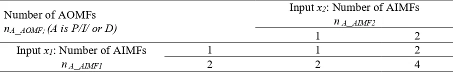
[image:15.595.85.538.493.565.2]U . In order words, the number of AIMFs and AOMFs can be then listed into four cases in Table 1.
Table 1
Active input MFs and corresponding active output MFs in fuzzy P/I/ Or D tuner.
Number of AOMFs
nA_AOMF; (A is P/I/ or D)
Input x2: Number of AIMFs n A_AIMF2
1 2
Input x1: Number of AIMFs n A_AIMF1
1 1 2
2 2 4
By utilizing Remark 5, each AIMF has only two parameters, a bj, j( orbj), and each AOMF
has one parameter, wk, which need to be optimized. Thus for each step of time, the decisive vector
size minimizer identifies three dynamic characteristic vectors, denoted as VPt, VIt, and VDt, for
15
/ / / /
11 11 21 21 12 12 22 22 1 2 3 4 max
/ /
11 11 21 21 1 min
Size of 1 12
Size of 1 5 , : , .
At size t
At size t
V a b a b a b a b w w w w
V a b a b w A P I or D
(34)
From (34), the total number of parameters which needs to be tune each step is reduced from (9(N1+N2)+3M) to the range [15, 36] disregarding the number of input/output MFs. Thus, the
decisive vector size minimizer could save remarkably the time to optimize the control parameters.
4.
Robust PI grey model-based prediction module
The RPIGM prediction module comprises two RPIGM predictors in which each predictor is constructed based on a main grey model (MGM, Section 4.1) integrated a PI-based weight tuner (PIWT, Section 4.2) to perform the prediction. Here, the PIWT is designed based on a Lyapunov stability condition and employed to regulate online the weight factors of the MGM with respect to the prediction error minimisation in order to ensure a robust prediction. The prediction procedure using the proposed RPIGM is then demonstrated in Fig. 3.
4.1. Main grey model
In grey prediction theory, GM(n, m) denotes the grey model, where n and m are the order and number of variables of the model. And GM(1,1) is known as the most popular grey model used for many practical applications [26]-[35]. With only a few historical data of the system output(s), the grey predictor can predict the future output(s) without knowing the mathematical model of the real system.
16
START
Prepare an object data Sequence using data rolling operation
Generate grey sequence, y(0) using:
+ recurrent signal
+ adaptive factors, c1 and c2
Generate a new sequence using accumulated generating algorithm, y(1)
Generate a background series using weighting factor, wPINN
Establish grey different equation & calculate [a, b] using least square estimation Setup prediction model & calculate model
output at step (n+p)th, y
raw(tn+p)
Stop working ?
STOP Calculate recurrent
signal: yraw(tn) = yraw(tn+1)
Y
N
Produce predicted object value for applications
Grey checking conditions to derive c1 and c2
(0)
Update prediction error function
PIWT robust controller using adaptive learning rates
Update weighting factor,
wPINN
^ ^
^
(0)-^ ^(0)
Learning rate selection based on Lyapunov stability condition
[image:17.595.108.499.99.477.2]Reference vector for prediction optimisation
Fig. 3. RPIGM prediction procedure using the MGM(1,1) integrated PIWT.
However, there exist some limitations in typical grey models which affect directly to their applicability as well as prediction accuracy:
Input raw data must be non-negative and satisfies the smooth condition (will be discussed later) to perform the grey model [25].
The background series of the model obtained using the MGO could cause internal errors in constructing the grey model [35].
There is no such condition or constraint to guarantee the model robustness.
17 precisely any signal, y, with random distribution. Using the grey theory, the MGM-based prediction procedure is built as demonstrated in Fig. 3 and, can be expressed as the following steps:
Step 1: Prepare an input grey sequence capable of approximating any system:
Prepare an sequence containing at least five latest data points of the object using the data rolling operation (discarding an oldest data and adding a newest data for each cycling time, [25]):
y
Objectt
O1,
y
Objectt
O2,...,
y
Objectt
Om
;
m
5
(35) Generate a raw input grey sequence with equal intervals from (35):
0
0
0
0
1 , 2 ,..., ; 5raw raw raw raw n
y y t y t y t n (36)
here, if the condition (37) holds, then sequence (36) is exactly similar to sequence (35); otherwise, sequence (36) is the sequence containing sequence (35) and new elements up to latest time point with the same intervals that are derived as (38) using the same MGM-based prediction.
11 1 1
/ 2; ; 2,...,
; : time of previous value of ;
Oi RGM Oi Oi O i
O O Olast Olast Object O
t T t t t i m
t t t t y t
(37)
here TMGM is the desired prediction sampling period;
0 0
1
1
ˆ ; ;
2,..., ; / ; 1,..., 1;
raw k raw k Oi k O i
Om RGM
y t y t t t t
k n n t t T i m
(38)
here * is the floor function to return nearest integer value.
To exhibit the dynamic temporal behaviour of the model, a recurrent signal as the one-step-ahead predicted value, denoted as 0
0
1
ˆraw n ˆraw n
y t y t , is added to the sequence. Thus, (36)
becomes:
0 0 0 0
1 2
0 0
, ,..., ; 6
ˆ .
raw raw raw raw n
raw n raw n
y y t y t y t n
y t y t
18 Remove the oldest elements from sequences (35) and (36). Then, generated a new series (40)
from (39) using Remark 6 to make it satisfy grey sequence checking conditions (41).
0 0 0 0
1 2
0 0
1 2
{ , ,..., }; 5
; 1,..., n
k raw k
y y t y t y t n
y t y t c c k n
(40)
0 0 1 0 1 01 , 1,..., 2 k k k i i i y t
y t k n
y t t
(41)Remark 6. By adding two non-negative additive factors c1 and c2 derived from (42) using the
previous work [35], the sequence (39) becomes (40) and satisfies the grey sequence checking conditions (41).
0 0 1 1,.., 1 0 0 1 1 12 1,.., 1
1
max , 0
2 max 0,
2 raw k raw k k n
k
raw k k raw i i
i k k n
i k
i
c y t y t
y t c t y t c t
c t t
(42)here,
is the small positive constant.Step 2: Generate a new series y(1) from y(0) using the AGO:
1 0 1 1 2 1, 1, 2,...,
k k i k raw k i
y k y i t k n
y i c c t
(43)Step 3: Instead of employing the MGO in typical grey models, the background series z(1) is newly
built from y(1) as:
1
1
1
1 1 ; 2,...,
k k k k k
z t w y t w y t k n (44)
19
1 1 2 1 2
1 1 1 2 1 2
0.5 1 1 1
0.5 1 1 1
k PINN PINN
k PINN PINN
w w w
w w w
(45)
where wPINN is called the adaptive gain and 0wPINN 1; in order to ensure the robust prediction, this adaptive gain is online regulated by the PIWT (Fig. 3) that is introduced in the next section;
1 2
{ , } is the set of activation factors and given as
0 0 0
1 1
0 0 0
1 2 1 1
ˆ
{1,0}, IF : ;
ˆ
{ , } {1,1}, IF : ;
{0,1},Others
raw k raw k raw k Object k
raw k Object k raw k raw k
y t y t y t y t
y t y t y t y t
(46)
Step 4: Establish the grey differential equation [25]
0
1
k k
y t az t b (47)
where a and b are the model parameters. By employing the LSM [25], the optimal values of the model parameters are obtained:
1ˆ
ˆ
ˆ
T T Tab
a b
B B B Y
(48)with
1 0 2 2 1 0 3 3 1 0 1 1 , . 1 n nz t y t
z t y t
B Y
z t y t
Step 5: By replacing the optimal solution (48) into (47) and using the recursive operation, the MGM(1,1) prediction is setup as follows:
0
1 1
0 1 1
3 2 2
ˆ ˆ 1 1 ˆ
ˆ ˆ ˆ 1 1 k i i k
i i i
t a t
b ay t t
y t
t a t t a t
(49)20
0
1 1
0 1 1
1 2
3
2 2
ˆ ˆ 1 1 ˆ
ˆ
ˆ ˆ
1 1
n p
i i
raw n p
i i i
t a t
b ay t t
y t c c
t a t t a t
(50)where p is the step size of the grey predictor.
4.2. PI-based weight tuner
In this section, the PI-based weight tuner is designed as the combination between PI algorithm, neural network and Lyapunov stability condition and integrated to the MGM to optimize online the adaptive gainwPINN in order to ensure the robust prediction.
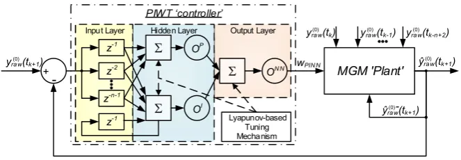
Remark 7. By considering the MGM-based prediction as a tracking control problem as described in Fig. 4, it is possible to derive a ‘robust controller’ PIWT to guarantee the closed-loop prediction stability of the ‘plant’ MGM.
z-1
z-2
z-n-1
S
S
ON N
OP
OI
S MGM 'Plant'
Lyapunov-based Tuning Mechanism z-1
-ŷraw(tk+1)
-+
PIWT ‘controller’
wPIN N
ŷraw(tk+1)
yra w(tk) yraw(tk-1) yra w(tk-n+2)
yraw(tk+1)
(0) (0) (0)
(0)
(0) (0)
[image:21.595.146.478.358.473.2]Input Layer Hidden Layer Output Layer
Fig. 4. Representative closed-control form to optimize the MGM using the PIWT.
Based on Remark 7 and Fig. 4, the PIWT is designed as the PI-type neural network structure with the Lyapunov stability condition. Here, the network consists of three layers: an input layer containing the prediction error sequence{ 0 ˆ 0 }
raw raw
y y , a hidden layer with two nodes following PI algorithm, and an output layer to compute the adaptive gain,wPINN. Define MGM { ,...,1 1}
k n
e e e 0 0
1
ˆ
1(
e y t
i
raw k i(
)
y t
raw k i(
), 1,...,
i
n
1)
is the input vector at step kth,{ Pi, Ii} k kw w are the weight
vectors of the hidden node P and I, respectively, and,{ P, I}
k k
21 1 1 1 1 1 :Node P :NodeI n
P Pi i
k i k k
n
I I Ii i
k k i k k
O w e
O O w e
(51)Then, the output from the network is obtained using the PI algorithm and sigmoid activation function:
1,
1 kNN
NN NN P P I I
PINN k O k k k k k
w f O O w O w O
e
(52)
The ‘controller’ output (52) is then fed into the ‘plan’ MGM (Section 4.1) to perform the prediction (as described in Fig. 3).
Next in order to ensure the robust prediction, the BP training algorithm based on a Lyapunov stability condition is utilized to tune the PIWT weights. Define a prediction error function:
2
21 0 0 1
1 1
1
ˆ
10.5
n0.5
nMGM i
k i raw k i raw k i i k
E
y
t
y
t
e
(53)Thus, the weight factors of the PIWT are online tuned for the next prediction step, (k+1)th,
using the delta rule:
/ / / / 1 / / / / 1 / /
P I P I P I MGM P I
k k k k k
Pi Ii Pi Ii Pi Ii MGM Pi Ii
k k k k k
w w E w
w w E w
(54)
where P I/ , Pi Ii/
k k
are learning rates within range [0,1]; the other factors in (54) are derived using the
partial derivative of the error function with respect to each decisive parameter.
Theorem 2. By selecting properly the learning rates Pi Ii/ P I/
k k k
for step (k+1)th to satisfy (55),
the stability of the MGM(1,1) prediction is guaranteed.
1 2 2
1 0.5 0
n i
k k k k k
i e F
F
(55) with 1 1 .j MGM j MGM
n
k k k k
k Pi Pj Ii Ij
j k k k k
e E e E
F
w w w w
22 Proof.Define a Lyapunov function as
2
21 0 0 1
1
ˆ
10.5
n0.5
nMGM i
k i raw i raw i i k
V
y
t
y
t
e
(56)By using the same method as presented in Appendix A according to (56), the MGM(1,1) prediction is guaranteed to be stable only if MGM1 0
k
V
. By selecting properly the learning rate to
satisfy (55), the sufficient condition for MGM1 0
k
V
is guaranteed. Therefore the proof is
completed.
4.3. Fuzzy grey cognitive map decision tool for RPIGM
A fuzzy cognitive map (FCM) is known as the neuro-fuzzy system which is graphically represented by a frame of nodes (input and output concepts) and connection edges between nodes to be capable of incorporating knowledge from experts [38]-[42]. With a traditional FCM, intensity of a causal relation between two concepts (weight) is set to zero in the adjacency matrix if this relation does not exist or is partial/completely unknown. Thus, a combination between FCMs and grey numbers can perform an effective decision making tool for solving problems within environments with high uncertainties and/or incomplete information.
In this study, an adaptive fuzzy grey cognitive map is newly designed in which the grey weights with dynamic bounds are used to build the map and online adjusted to minimize a pre-defined cost function. This FGCM is then used to tune the RPIGM prediction step size.
a) FGCM design
By using the grey theory [25], the FGCM is generally designed for a set of NC concepts and,
therefore, can be represented by
,
,
C
i ij
C t
w t f
(57)whereC ti( )is the grey value of ith concept defined in (58); ( )
ij
w t
is the grey weight between
concept ith and jth defined in (59); fC(*) is the activation function defined in (60) ( is the steepness
23
( ) [ ( ), ( )] ([0,1]or[ 1,1]),
i i i
C t C t C t
(58)
( ) [ ( ), ( )] ([0,1] or [ 1,1]),
ij ij ij
w t w t w t
(59)
(*) 1
(*) (*) (*) (*) 1
(1 ) , (*) 0,1 ,
*
( )( ) , (*) 1,1 .
C e if
f
e e e e if
(60)
Remark 8. Bounds of grey numbers in the FGCM (concepts’ values and weights) are properly initialized within the maximum range [0,1] or [-1,1]. These bounds are adjustable online but limited to their maximum ranges.
By using FCM theory and Remark 8, the grey value of each concept can be updated for each step of time based on the influences of the other interconnected concepts:
1, 1
1 , 1 0,1 or 1,1
N C
i i j j i ji j
i i
C t f C t w t C t
sat C t C t
(61)
where sat(*) is the saturation function of *.
b) FGCM training algorithm
In order to increase the decision accuracy of the FGCM when dealing with partial unknown systems and uncertainties, the grey weights are updated online using the nonlinear Hebbian-type learning rule [42]:
1
1 , 1 0,1 or 1,1
ji ji ji
ji AFGCM j i ji j
ji ji
w t w t w t
w t C t C t w t C t
sat w t w t
(62)
hereAFGCMis the learning rate.
Remark 9. The FGCM grey weights are updated until one of the two following termination conditions are achieved:
24
2min min
1 i , 0
m des des
d i
i
J
C C J J (63) Minimum changing speed of decisive concepts’ values:
1
,
1,..., ,
0
des des
i i C C
C
t
C
t
i
m
(64)where
i
des d
C is the desired value of the decisive concept ith, des i
C ; m is the number of decisive
concepts; Jmin is the desired cost;Cis the small constant.
4.4. Utilization of RPIGM with FGCM for system response estimation
By utilizing the designs of MGM(1,1), PIWT and FGCM, the first predictor, tagged as RPIGM1,
is constructed to derive the filtered value of the system response at the current step,
y t
ˆ
( )
y t
ˆ
raw n 0( )
, and its estimated value at p-step ahead,
y t p
ˆ
(
)
y t
ˆ
raw n p 0(
)
. The filtered response is sent to thesecond predictor, tagged as RPIGM2, to produce the compensative control signal while the predicted future response is sent to the RFPID module to optimize its control parameters (Section 3). Generally, the purpose is to design a controller to achieve a good tracking performance. In other words, the control system should be built in order to speed up the system response (or reduce the rising time), and reduce the steady state error (or increase the control precision).
Remark 10. In a control system using grey predictor, the prediction step size (p) affects directly on the system performance. During the rising time period, with a small value of p the predictor speeds up the system response but causes the large overshoot or oscillation. Otherwise when the system is closed to the desired state, the predictor with a large value of p reduces the overshoot but increases the rising time [16].
25
4.5. Utilization of RPIGM for control compensation of noises and disturbances
As presented in Section 4.3, the RPIGM2 receives the filtered response, output from the RPIGM1, to estimate the influences of noises and disturbances on the system performance at the following step and, consequently, to create properly the additive correction to the main control signal (as in (1)) to compensate for these undesirable influences.
Here, the data sequence input to the model is the amount of system response, eND, caused by
the noises and disturbances as
_ _ _ _
_
0 0 0 0
1 2
0 0 0
, ,..., , 5
ˆ , 1, 2,...,
ND raw ND raw ND raw ND raw ND ND raw
n ND
k raw k raw k ND
e e t e t e t n
e t y t y t k n
(65)
here
y t
raw k 0( ) and
y t
ˆ
raw k 0( )
are in turn the measured system responsey t
( )
and its filtered valuey t
ˆ( )
using the RPIGM1 at step kth.
The impacts of noises and disturbances on the system at the coming step of time, (n+1)th, is
then estimated using (50) as
_
0 1
1 1
0 1 1
1 1 2
3
2 2
ˆ ˆ 1 1 ˆ
ˆ
ˆ ˆ
1 1
ND ND raw ND
n
ND i ND i
ND ND ND
n ND ND
i
ND ND ND i ND i
t a t
b a e t t
e t c c
t a t t a t
(66)Finally, the additive control signal with respect to the estimated influence of perturbations on the system at the coming step, (t+1)th, shown in (3) can be derived by using the result in (66).
5.
Illustrative Examples
5.1. RPIGM prediction module evaluation
a) Case study 1 – Prediction accuracy
PIWT-26 integrated MGM(1,1)), was carried out to perform one-step ahead estimation (p = 1) of communication delay problem in the networked system introduced in [35]. The functionalities of these models can be summarized in Table 2.
Table 2
Functionalities of comparative grey models.
Grey model
Functionalities
Input data Data intervals Background series
Prediction error minimisation GM Only data
satisfying checking conditions
Must be equal intervals
Use MGO No
SAUIGM Work with any data Work with unequal intervals
Use modified MGO (exact solution)
Use lth-order error correction accumulation RPIGM Work with any data Work with
unequal intervals
Use modified algorithm with adaptive weights
Use PIWT with Lyapunov
[image:27.595.93.535.217.557.2]stability condition
Fig. 5. Experimental setup to detect communication delays of the networked system [35].
27 functions is capable of, first, measuring accurately the real working time of the system and, second, recognizing the networked communication delays [35].
[image:28.595.181.443.322.518.2]To investigate only the communication delay through this networked setup and due to the applicability of the GM limited to equal-time-interval time series, a simple program with the fixed sampling period of 10ms was built in the Simulink environment combined with Real-time Windows Target Toolbox of Matlab to send a random signal to the coordinator during 30 seconds. This signal was then transmitted to the router by the ZigBee protocol. Once receiving the information from the coordinator, the router immediately sent a random signal back to the coordinator to perform the simple closed-loop networked system. The three grey models were then applied to forecast the time delays over the testing period.
Fig. 6. Real-time delay predictions vs. actual delays.
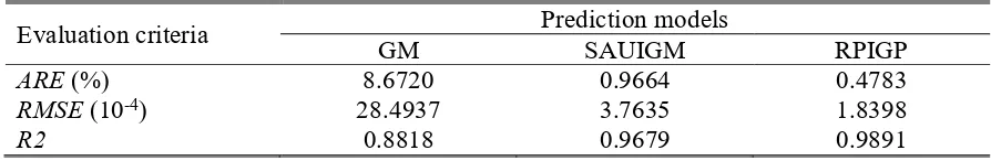
Table 3
Real-time delay predictions using different models.
Evaluation criteria GM Prediction models SAUIGM RPIGP
ARE (%) 8.6720 0.9664 0.4783
RMSE (10-4) 28.4937 3.7635 1.8398
R2 0.8818 0.9679 0.9891
[image:28.595.87.534.594.667.2]28 accuracy using the typical GM as shown in the top sup-plot of Fig. 6 was low due to its drawbacks (stated in Section 4.1 and Table 2). By applying the SAUIGM with the exact solution to compute the background series and lth-order error correction accumulation [35], the performance was significantly improved (see the middle sub-plot). However, there was no sufficient condition to ensure the robust prediction. Meanwhile, by employing the RPIGM, which was constructed based on the PIWT using the PI-based neural network and Lyapunov condition, the robust prediction with the highest accuracy could be achieved as presented in the bottom sub-plot.
Three evaluation criteria, average relative error (ARE), root mean square error (RMSE), coefficient of determination (R2), were employed to evaluate the performances of the grey models:
(0) (0)
(0) 1
ˆ 1
(%) n raw raw 100
k raw
y k y k
ARE
n y k
(67)
(0) (0)
21 1
ˆ
n
raw raw
k
RMSE y k y k
n
(68)
2 (0) (0) 1
2 (0)
1
ˆ 2 1
n
raw raw
k n
raw k
y k y k
R
y k y
(69)where y in this case if the communication delay;
y
is the mean value of this delay observation.The model evaluation was then carried out as shown in Table 3. The results confirmed that the best prediction performance was enhanced by the RPIGM.
b) Case study 2 – Prediction stability
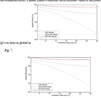
29 the estimation results, a model fitness evaluation versus different values of the prediction step size
(p) was done as plotted in
Fig. 7.
Fig. 7. Fitness evaluation on the delay prediction models.
The result shows that the GM-based estimation accuracy was continuously reduced according to the step size increase (indicated by the black dot line). Although the SAUIGM could improve the accuracy with the error correction accumulation (the blue dash-dot line), its performance was also degraded due to the lack of stability constraint. Only by utilizing the RPIGM with the robust stability condition, the high accuracy could be well maintained as (the red solid line) or, the stable estimation was guaranteed.
5.2. RPTC tracking control evaluation
[image:30.595.82.480.110.495.2]30 control robustly. The EMLS includes a sphere barium-strontium magnet (2.54mm of diameter), a ferrite-core coil to position the magnet, and a 50V/T Hall effect sensor to observe the magnet position. The driving coil and hall sensor are installed vertically and fixed on a frame to create the moving space for the magnet. The magnet can be levitated in mid-air with an impressive air gap about 25mm using a Hilink real-time multi-function card [44].
The Hilink platform offers a seamless interface between a physical plant and Matlab/Simulink via a serial communication port. This is fully integrated into Matlab/Simulink and comes with a specific Hilink library blocks associated with hardware inputs and outputs. It therefore allows quick configuration of control strategies in real-time with a real plant in the loop. The platform achieves real-time operation with sampling rates up to 3.8kHz [44]. Here, the EMLS control signal is sent from the high performance PC installed Matlab/Simulink through the Hilink board. The magnet movement is managed and represented by the Hall sensor signal which is fed-back to the PC through the card to perform the closed-loop control system.
To evaluate the control effectiveness, the proposed RPTC scheme was compared with other four control methods in driving the magnet of the EMLS. The compared controllers were a PID controller and three advanced controllers: fuzzy PID (FPID), fuzzy PID based on an online tuning grey predictor [16] (OTGFPID1), and online tuning fuzzy PID based on an online tuning grey predictor in which the grey model was the SAUIGM model developed in [35] (OTGFPID2). The advantages of these control methodologies over conventional techniques have been proven in [9] and [16].
31 (b) Configuration of the EMLS
Fig. 8. Configuration of EMLS system with real-time tracking control.
Z VS S M B
0.5 0.75 1
0 0.25 1.25
-0.25
|e*(t)| |de*(t)|
or
(a) Initial MFs for the inputs:
e t
*
,de t
*
VS S M B
Z
0.75 1
0.25 0.5 0
UAFuzzy
(b) Initial MFs for the output: Fuzzy A
U (A is P, I, or D)
Fig. 9. Initial MFs of the inputs/outputs of fuzzy tuners: P, I, or D.
For simplicity in making the comparison with the developed controllers, the fuzzy tuner designs of the RFPID control module of the RPTC were followed the designs in [9] and [16]. Thus, each
the fuzzy tuner contained two inputs,
e t
*
andde t
*
, and one output Fuzzy AU (A is P, I, or D).
[image:32.595.180.451.291.494.2]32 Next, the designs and setting of the four comparative controllers were considered. With the PID controller, the PID gains were derived through a two-step procedure in Matlab/Simulink: first, the EMLS model developed in [43] was employed to represent the real system and their model parameters were optimized using the parameter estimation toolbox, and second, a closed-loop control simulation with the optimized model and the PID controller was performed to optimize the PID gains using the PID tuning toolbox. The last FPID, and OTGFPID1 and OTGFPID2 controllers were constructed with the same fuzzy PID design as that of the RPTC except the use of the robust learning mechanism (Section 3.2). In addition, the fuzzy PID parameters of the OTGFPID2 was online tuned by the delta rule-based learning mechanism in [9]. For the prediction functions, the typical grey model, GM(1,1), of OTGFPID1 and the SAUIGM model of OTGFPID2 used the same method proposed in [16] to tune the prediction step size.
Table 4
Rules table of RFPID control module.
Fuzzy Outputs
( Fuzzy, Fuzzy, Fuzzy)
P I D
U U U
*
de t
Z VS S M B
*
e t
Z VS,B,M VS,B,M Z,B,M Z,B,B Z,B,B
VS VS,B,S VS,B,M VS,B,M Z,M,M Z,M,B
S S,M,VS S,M,VS S,M,VS VS,S,S VS,S,S
M M,Z,Z M,Z,Z M,VS,VS S,VS,VS S,VS,VS
B B,Z,Z B,Z,Z B,Z,Z B,Z,Z M,Z,Z
The controllers were built in the Simulink environment combined with Real-time Windows Target toolbox. The sampling rate was set to 1ms. In addition, to evaluate the system stability, a noise source (N) and a disturbance source (D) were generated and in turn added to the controllers’ outputs and the Hall sensor feedback signal (Fig. 1) as
( ) N[ Nsin(2 N ) Rand ( )]N
N t k A f t t
here AN was given randomly from -1 to 1; fN was varied from 1 to 5 Hz; RandN is the noise signal
with power 0.5; kN = 0.02; and:
( ) D[ Dsin(2 D ) D( )]
33 where
1 : 0 ( mod )
( ) , 0 1
0 : ( mod )
D D D
D D
D D D D
IF t T p T
x t p
IF p T t T T
here AD was the Gaussian distribution with mean 0.01 and variance 0.1; fD was varied from 1 to 0.1
Hz; xD is the pulse wave signal with the pulse width, pD, set to 30% of the signal period TD = 2 s;
and kD = 0.02.
The control target was to drive the magnet to follow a given trajectory defined as the distance from the coil to the magnet. The best working position of the magnet was around a distance of 20mm from the end surface of the driving coil. The real-time tracking control tests on the EMLS were then carried out to validate the applicability of the comparative approaches.
18 19 20 21 22 23
M
ag
ne
t
D
is
pl
ac
e
m
e
nt
[m
m
] 1
2
3 4
5 5
0. Reference ; 1. PID; 2. FPID ; 3. OTGFPID1; 4. OTGFPID2; 5. RPTC
0 2 4 6 8 10 12 14
-0.4 -0.2 0.0 0.2 0.4
Time [s]
T
ra
ck
in
g
E
rr
or
[m
m
]
4
3
Fig. 10. EMLS multi-step tracking performances with different controllers.
[image:34.595.182.445.349.634.2]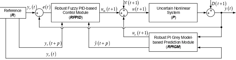


![Fig. 5. Experimental setup to detect communication delays of the networked system [35]](https://thumb-us.123doks.com/thumbv2/123dok_us/9428751.447865/27.595.93.535.217.557/fig-experimental-setup-detect-communication-delays-networked.webp)