Viscous effects on the attenuation of a plane wave by an acoustic lining in shear flow

Original citation:

Khamis, Doran and Brambley, Edward J. (James). (2017) Viscous effects on the attenuation

of a plane wave by an acoustic lining in shear flow. The Journal of the Acoustical Society of

America, 141 (4). pp. 2408-2417.

Permanent WRAP URL:

http://wrap.warwick.ac.uk/94085

Copyright and reuse:

The Warwick Research Archive Portal (WRAP) makes this work by researchers of the

University of Warwick available open access under the following conditions. Copyright ©

and all moral rights to the version of the paper presented here belong to the individual

author(s) and/or other copyright owners. To the extent reasonable and practicable the

material made available in WRAP has been checked for eligibility before being made

available.

Copies of full items can be used for personal research or study, educational, or not-for-profit

purposes without prior permission or charge. Provided that the authors, title and full

bibliographic details are credited, a hyperlink and/or URL is given for the original metadata

page and the content is not changed in any way.

Publisher’s statement:

Copyright © 2017 Acoustical Society of America. This article may be downloaded for

personal use only. Any other use requires prior permission of the author and the Acoustical

Society of America.

The following article appeared in Khamis, Doran and Brambley, Edward J. (James). (2017)

Viscous effects on the attenuation of a plane wave by an acoustic lining in shear flow. The

Journal of the Acoustical Society of America, 141 (4). pp. 2408-2417 and may be found at

http://dx.doi.org/10.1121/1.4979469

A note on versions:

The version presented here may differ from the published version or, version of record, if

you wish to cite this item you are advised to consult the publisher’s version. Please see the

‘permanent WRAP URL’ above for details on accessing the published version and note that

access may require a subscription.

Viscous effects on the attenuation of a plane wave

by an acoustic lining in shear flow

Doran Khamis

and Edward James Brambley

1

DAMTP, University of Cambridge, Cambridge, UK

J. Acoust. Soc. Am.141_{(4), pp. 2408–2417 (2017),doi:10.1121/1.4979469.}

Received 29 October 2016; revised 30 January 2017; accepted 17 March 2017; published online 6 April 2017

Abstract

The attenuation of a plane acoustic wave incident on a flat impedance surface in a sheared and viscous fluid is investigated numerically and asymptotically. Predictions of various bound-ary models of impedance surfaces in shear flow are tested by comparing their predicted re-flection coefficient. It is found that viscosity has a significant effect, reducing the rere-flection of upstream propagating sound while increasing the reflection of cross-stream propagating sound. The classical Ingard–Myers boundary condition is shown to incorrectly predict the damping rate of sound in many cases, and in some cases viscous effects are shown to be comparable to shear effects.

I

Introduction

Wave propagation in a steady flow over an acoustically lined wall has been widely studied due to its applications to noise damping in acoustically lined aeroengines. So that noise damping predictions may be useful, any simplified acoustic boundary condition used must have the correct attenuation properties. Gabard (2013) tested a range of inviscid impedance boundary conditions by the benchmark problem of a plane wave incident on a shear layer above a lined wall. Numerical solutions of the Pridmore-Brown(1958) equation were compared with analytical expressions for the reflection coefficients obtained using the Myers boundary condition (Ingard,1959,Myers,1980) and its various first order corrections (Rienstra and Darau,2011, Brambley, 2011). It was found that the thickness of the boundary layer can significantly affect the reflection coefficient, and that use of the Myers condition can lead to large errors in sound attenuation predictions (Gabard,2013). Recent work has suggested that, to reconcile theoretical predictions with experimental results, viscous effects need to be taken into account (Burak et al., 2009, Renou and Aur´egan, 2011). It was shown in Khamis and Brambley (2017) that viscosity and thermal conduction can play a large role in the damping rate of cut-on modes, and that viscosity can be as important as shear in some circumstances. The experimental results ofMarx et al. (2010) were inaccurately repro-duced by the invsicid numerics in Boyer et al. (2011). The computations of Marx and Aur´egan

(2013) did include viscous effects and it was shown that the wave mode found in the experimental study (Marx et al.,2010) is particularly sensitive to viscosity.

In this paper the work of Gabard (2013) is extended to account for viscothermal effects. A numerical method is proposed for computing the reflection coefficient of a plane wave incident on sheared viscous boundary layer above an acoustic liner. The numerical method is used to compare the reflection coefficient with and without viscosity, and to measure the accuracy of simplified analytical expressions for the reflection coefficient derived from an assortment of inviscid (Ingard,

1959, Myers, 1980, Brambley, 2011, Khamis and Brambley, 2016a) and viscous (Aur´egan et al.,

2001, Khamis and Brambley, 2017, 2016b) effective impedance boundary conditions. The My-ers (Ingard, 1959,Myers, 1980) boundary condition assumes an infinitely thin inviscid boundary

a) b)

Figure 1: The arrangement of the angles defining the incident and reflected wave directions with respect to the coordinate directions. Adapted fromGabard(2013).

layer, while the first order (Brambley, 2011) and second order (Khamis and Brambley, 2016a) corrections to the Myers boundary condition account for a finitely thick region of shear by de-riving matched asymptotic expansions in the inviscid boundary layer. Aur´egan et al.(2001) were the first to include viscosity in an impedance boundary condition (henceforth ASP), but assumed a low Mach number to reach a simple analytical result. The high-frequency boundary condi-tion (Khamis and Brambley,2017) accounts for a finitely thick viscous boundary layer by assuming a scaling relationship between the high frequency (ω) and thin boundary layer (δ),δ∼ω−3/2_{, and}

deriving a multiple scales solution inside the boundary layer. In contrast, the two-deck boundary condition (Khamis and Brambley,2016b) is derived using matched asymptotic expansions across a boundary layer that consists of a weakly viscous outer deck whereδ∼Re−1/3_{, and a fully viscous}

inner deck that has the acoustic boundary layer scalingδac∼(ωRe)−1/2.

II

Mathematical formulation

The situation considered is sketched in fig. 1. We consider a Cartesian coordinate system x ₌

(x, y, z) with a mean flow U _{= (U(y),0,0) and mean temperature and density T(y) and ρ(y),}

respectively, above an acoustically lined wall situated aty= 0 for all xand z. Above some point

y ∼δ > 0, the mean flow is uniform, such thatU(y) =U0, T(y) =T0 and ρ(y) =ρ0 for y &δ

(the free stream). Below this point, the mean flow follows some sheared profile down to the wall upon which no slip is satisfied. We define the dimensionless Reynolds and Prandtl numbers as Re =c0lρ0/µ0, and Pr =µ0cp/κ0, wherec0 is the speed of sound in the free-stream,lis a

length-scale (such as a duct width),cp is the specific heat capacity at constant pressure, andµ0 andκ0

are the coefficients of shear viscosity and thermal conductivity, respectively, in the free-stream. In the uniform flow region, the acoustic velocity potential, ˜φ, satisfies the convected wave equation

1

c2 0

D2_φ˜

Dt2 −∇

2_{φ˜= 0, (1)}

whereD/Dt=∂/∂t+U ∂/∂xis the material derivative. A monochromatic plane wave solution of (1) is

˜

φ= ei(ωt−Kθ_i·x)

+Rei(ωt−Kθ_r·x)

, (2)

where θ_{i and}θ_{r are unit vectors giving the directions of the incident and reflected plane waves}

respectively,K =ω/(c0D) is the acoustic wavenumber,D = 1 +Mθi·ex is the Doppler factor,

M = U0/c0 is the mean flow Mach number, and R is the reflection coefficient. We may derive

other acoustic quantities from ˜φusing

˜

u₌∇_φ,˜ _p˜=−ρ0Dφ˜

Dt, T˜=

˜

p cpρ0

. (3)

The vectorsθ_{i and}θ_{rare defined as}

θ_{i= sinαcosβ}e_x−cosαe_{y+ sinαsinβ}e_{z, (4a)}

in three dimensions, and θ_{i = cosθ}e_x−sinθe_{y, and} θ_{r = cosθ}e_{x+ sinθ}e_{y in two dimensions}

(see fig.1). In 3D the Doppler factor isD= 1 +Msinαcosβ, while in 2D the Doppler factor is

D= 1 +Mcosθ. For convenience, We defineKθ_r=kxe_x+kye_y+kze_z.

II.A

Asymptotic reflection coefficients

Here, we consider continuing the uniform flow solution (1) to y = 0 and applying an effective impedance boundary condition that incorporates the actual impedance Z of the lining and the effects of shear and viscosity within the boundary layer over the lining. FollowingGabard(2013), the effective impedance boundary conditions may usually be expressed in the form

˜

p(0)

−˜v(0) =Zeff =

ω ω−U0kx

Z+iQ0ρ0(ω −U0kx)

2 ωky

1−iQ1_ρ0Zc0

, (5)

where ˜p(0) and ˜v(0) are the pressure ˜pand the normal velocity˜u_·e_{y evaluated at the liningy= 0.}

The as yet arbitrary functions Q0 and Q1 may depend on, in general: the mean velocity and

temperature profilesU(y) andT(y); the modal wavenumberskx,ky andkz, and the frequencyω;

and the Reynolds and Prandtl numbers Re and Pr. Making use of the identities

ω−U0kx=c0K,

ω

ω−U0kx =D, (6)

we find ˜p(0) =−iρ0c0K(R+ 1) and ˜v(0) =−iky(R−1), which, when substituted into (5), lead to

R=

Z ρ0c0(D

θ_r·e_{y+iQ1)−1 +iQ0}

Z ρ0c0(D

θ_r·e_{y−iQ1) + 1 +iQ0}. (7)

Rederiving the second-order inviscid boundary condition (Khamis and Brambley, 2016a) for the flat Cartesian geometry considered here leads to (5) with

Q0=Dθr·ey

h

−K

DδI0−i(δI0δI1+δ

2_I

3−δ2I10)K⊥2

Z ρ0c0

+i K2−K⊥2

δ2I00

Z ρ0c0

i

, (8a)

Q1=−K 2 ⊥D

K δI1+i(δI0δI1+δ

2_I

11−δ2I01)K 2 ⊥ρ0c0

Z −i K

2_−K2 ⊥

δ2I2ρ0c0

Z (8b)

whereK2

⊥=kx2+k2z. The integralsIj are defined by

δI0=

Z ∞

0

χ0dy, δI1=

Z ∞

0

χ1dy, δ2I2=

Z ∞

0

yχ0dy, δ2I3=

Z ∞

0

yχ1dy,

δ2I01=

Z ∞

0

χ0

Z y

0

χ1(ˆy)dˆydy, δ2I10=

Z ∞

0

χ1

Z y

0

χ0(ˆy)dˆydy, (9)

δ2_I 00=

Z ∞

0

Z y

0

χ0(ˆy)dˆy−I0

dy, δ2_I 11=

Z ∞

0

Z y

0

χ1(ˆy)dˆy−I1

dy.

with

χ0(y) = 1−ρ(y)(ω−U(y)kx) 2

ρ0(ω−U0kx)2

, χ1(y) = 1− ρ0(ω−U0kx) 2

ρ(y)(ω−U(y)kx)2

. (10) The reflection coefficient for the high-frequency viscous model (eq. (5.13) ofKhamis and Brambley,

2017) may be defined by the parameters

Q0=θr·ey

hiT(0)

T0

r _µ

0

iωρ0

kxU′(0)

ρ0c20K

Z−KδI0−iDB

Z ρ0c0

i

, (11a)

Q1=−

K2 ⊥D

K δI0+ iρ0c0

Z A+iC, (11b)

where a prime denotes a derivative with respect toy, and

A=K⊥2(δI0δI1+δ

2_I

11−δ2I01)−(K2−K⊥2)δ 2_I

2, (12a)

B=K⊥2(δI0δI1+δ2I3−δ2I10)−(K2−K⊥2)δ

2_I 00

+µ0T(0)

2

iωρ0T02

1

T(0)2

Iµ

δ2 +

2σ

1 +σ U′

(0)2

cpT(0)

−5k

2 x

4ω2U ′

(0)2

, (12b)

C=T(0)

T0 r _µ 0 iωρ0 −K 2 ⊥ K2

ikxU′(0)

c0 δI1+

ic0

ω ρ0

ρ(0)K

2 ⊥+

iωcpT0

σc3 0

andσ2_{= Pr. The viscous integralI}

µ/δ2is defined by

1

δ2Iµ=

Z ∞

0

χµdy, χµ=

ω ω−U kx

h 1

2 Pr(T

2₎

yyy+cp(T U

′2₎′

+ kxT

ω−U kx

(T U′

)yy

i

. (13)

For the two-deck viscothermal boundary condition (Khamis and Brambley, 2016b), the Qj

parameters are

Q0=θr·ey

iT(0) T0 r _µ 0 iωρ0

kxU′(0)

ρ0c20K

Z−KδI0−iD(S2+S3) Z

ρ0c0

, (14a)

Q1=−K 2 ⊥D

K δI1+iC, (14b)

where

S2=µ0T(0) 2

iωρ0T02

1

T(0)2

Iµ

δ2 +

2σ

1 +σ U′

(0)2

cpT(0)

− 5k

2 x

4ω2U ′

(0)2

, (15a)

S3=

_T(0) T0 r _µ 0 iωρ0 3

−cpkxU

′

(0)

c2 0ωT(0)

Iµ

δ2 −

13k2 x

8ω2 U ′

(0)U′′

(0)−k

ωU

′′′

(0)− T ′′′

(0)

σPrT(0)

−151k

3 x

32ω3 U ′

(0)3+(7σ+ 3) (1 +σ)2

kxU′(0)3

2cpωT(0)

+(σPr + Pr−2σ−1)

σ(1 +σ)2

2U′

(0)U′′

(0)

cpT(0)

(15b)

−(2 Pr +4σ+ 1)

(1 +σ)2

kxU′(0)T′′(0)

ωT(0)

.

To rewrite the boundary condition equation (23) of Aur´egan et al. (2001) in a useable form, we first exchange Yc with Y (correcting a typographic error in the reference) and then identify

Yc = 1/Zeff. Ignoring the acoustic boundary layer term premultiplied by δa as suggested in the

paragraph following equation (23) of that reference, we findQ0= 0 and

Q1=iρ0c0

Z

βvU0kx

ω−U0kx

+ ω

ω−U0kx

T0−T(0)

T(0) βt

, (16)

where

βv =

1 U0 Z ∞ 0 dU dye

−_(1+i)wy/δa

dy βt=

1

T0−T(0)

Z ∞

0

dT dye

−_{(1+i)σwy/δa}

dy, (17)

where the complex conjugate is taken due to our different choice of sign in exp(+iωt). Aur´egan et al.

(2001) modelled the fluid as having constant viscosity, but since the viscosity here isy dependent due to varying mean flow temperature (19), we find best agreement with our numerics is given using the viscosity at the boundary, givingδa= (2µ(0)w/ρ(0)c20)1/2.

II.B

Computational method

The computational domain is taken to be y ∈ [0, yn] whereyn = 2πn/ky is chosen such that n

wall-normal uniform-flow wavelengths fit within the domain. The lined wall is situated aty= 0, and a non-uniform gridyi,i= 1,2, ..., N (with more points clustered near the wall to fully resolve

the boundary layer) is mapped to a uniform computational gridξi via the mapping

ξi=

yn A arcsinh _y i yN sinhA , (18)

for a real-valued parameterA that governs the severity of the grid stretching. The parameters

N = 104_{, A = 8.5 andn = 3 were found to give stable, well-converged results (independent of}

total grid and step sizes), and were used in all the following computations.

The linearised compressible Navier–Stokes equations (LNSE) are solved within the domain using a 6th order maximal order finite difference scheme to approximate derivatives with respect to y (reducing to a 4th order scheme near the domain boundaries). The viscosities (shear and bulk) and thermal conductivity are modelled as having a linear dependence on the temperature, such that

µ∝µB ∝ T

T0Re

, κ∝ T

T0Re Pr

A ratioµB

0/µ0= 0.6 is used for all computations (Cramer,2012). A sheared mean flow profile is

applied, with the mean velocityU and temperatureT having the forms

U(y) =U0tanh

4y

δ , T(y) =T0+TBLsech

4y

δ , (20)

where T0 is the free-stream temperature andTBL ≈0.26T0 is used here to approximates a

com-pressible Blasius profile wall temperature.

An incident inviscid plane wave of unit amplitude is injected at the top of the domain using the boundary condition

˜

φ′

+ikyφ˜= 2ikye

−iKyNθi·e_y

. (21)

Since this is an inviscid plane wave and we are only interested in the effects of viscosity within the boundary layer, viscous effects are smoothly but rapidly “turned off” at the top of the boundary layer when the velocity and temperature reach their free-stream values. Were the effects of viscosity outside the boundary layer to be included, the incoming plane wave would decay slightly due to viscosity before entering the boundary layer, and the results would depend on the vertical distanceyn the wave travels before encountering the boundary. Turning off viscosity is achieved

by multiplying the viscous terms by the sigmoid-type function

hµ(y) =







1, y < ys,

2− 2

1 + exp (−b(y−ys)), y > ys,

(22)

wherey=ys marks the edge of the shear layer (taken here to beys≃4.77δ) andb≈60 governs

the speed at which the functionhµ approaches zero aboveys.

The reflection coefficient is calculated from the amplitude of the inviscid reflected wave at the top of the domain, given by the complementary expression to (21)

˜

φ′

−ikyφ˜=−2ikyRe−ikyyN. (23)

Applying this boundary condition to each of the five LNSE variables yields five reflection coeffi-cients,

Ru=−(2kxky)

−₁

eikyyN _u˜′_(y

N)−ikyu˜(yN), Rv=−(2k2y)

−₁

eikyyN _v˜′_(y

N)−ikyv˜(yN),

Rw=−(2kzky)−1eikyyN w˜′(yN)−ikyw˜(yN), (24)

Rp=−(2Kky)

−1_eikyyN _p˜′_(y

N)−ikyp˜(yN)

, Rt=−(2Kky)

−1_eikyyN _T˜′_(y

N)−ikyT˜(yN)

.

These should all result in the same numerical value, forming a useful test of the numerical method. The standard deviation1_{of theR}

j values in the test cases presented here was of the order of 10−8,

meaning error bars would be invisible in the following plots and have hence been omitted. Taking the mean of theRj from (24) then gives us the value ofRwhich we compare with the asymptotic

approximations, given above. The inviscid numerical results are obtained using the same viscous numerics by settingµ= 0.

III

Results

Here we plot results for the reflection coefficient of a plane wave incident on a boundary layer above a lined wall at any angle in two and three dimensions. The three viscous asymptotic expressions (11), (14) and (16) are compared to the viscous numerics; the inviscid second order expression (8) is compared to the inviscid numerics; and the viscous numerics are compared to the inviscid numerics. Also plotted are the reflection coefficients found using the Ingard–Myers (Ingard,1959,

Myers, 1980) condition and its first order correction (Brambley,2011). The reflection coefficient of the Myers condition is defined by (7) with Q0 = Q1 = 0. The first order inviscid boundary

condition is defined by (7) withQ0=−kyδI0 andQ1=−K⊥2DδI1/K.

We give results for the five test cases considered byGabard(2013), listed in table1; these cases are intended to be typical of a turbofan engine duct.

1_{Standard deviation defined here asσ}2 SD =

1

NRΣ(|

R_{j| − |}R_µ|)2_{, whereN}

Case Frequencyω/c0 Shear thicknessδ Mach numberM ImpedanceZ/ρ0c0

A 28 14×10−3 _{0.55 5−i}

B 28 7×10−3 _{0.55 5−i}

C 56 14×10−3 _{0.55 5−i}

D 28 14×10−3 _{0.3 5−i}

E 28 30×10−3 _{0.55 3−0.5i}

Table 1: Test cases for reflection coefficient calculations, as used inGabard(2013).

Gabard(2013) reports that case A corresponds to the near-fan flow conditions at the inlet of a turbofan engine at blade passing frequency; case B represents the flow upstream of the fan where the boundary layer would be thinner; case C tests the double frequency harmonic of the blade passing frequency; case D tests a lower Mach number flow; and case E corresponds to the thicker boundary layer and altered impedance of the bypass duct.

III.A

Two dimensions

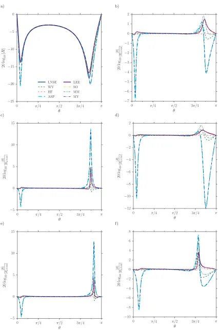
In this section we constrain the incident wave to lie in the same plane as the direction of the mean flow, as in fig.1b. The angle θ is varied between 0 andπ, so that the wave is incident anywhere between directly downstream and directly upstream. Figure 2 shows results at high Reynolds numbers for the reflection coefficient for the five cases listed in table 1. Figure 2a shows the absolute reflection coefficient in decibels for case A. Since it is difficult to compare between results on this scale, figs.2b–2fplot the reflection coefficient relative to the LNSE reflection for cases A–E. All the models agree when the incident wave is perpendicular to the mean flow. In all cases, the greatest discrepancy between inviscid and viscous reflection comes when the wave is incident in an upstream direction. This could be explained by the refraction of upstream propagating waves away from the lining by the mean flow shear (Allen et al., 2013, pg. 34–40), and the resulting increase in the relative importance of viscosity to the attenuation rate (Stokes, 1845) due to a reduced interaction with the lining. This feature is well captured by the high frequency asymptotic solution, and partially captured by the two-deck weakly viscous model. We also recover the result ofGabard(2013) that the Myers boundary condition is ill-suited for attenuation calculations, with the reflection coefficient of waves incident at shallow angles being predicted with errors of up to 10 dB with respect to inviscid numerics. Viscosity is seen to have a non-negligible effect on the reflection coefficient of around 1.5 dB to 4 dB. The leading-order ASP boundary condition does not fare better than the Myers condition, despite including viscosity, possibly since the moderate Mach numbers used here are too high for the low-Mach-number assumption of ASP.

Figure 3 shows results for lower Reynolds numbers. As intuition suggests, this separates the viscous and inviscid models by a greater amount, particularly for upstream propagating waves. In figs.3b,3dand3f the benefits of using the second-order accurate inviscid boundary condition over the first-order inviscid boundary condition for inviscid calculations may be seen, with the first order condition having errors of more than 1 dB for upstream propagating incident waves compared to the LEE numerics. The second order inviscid condition consistently predicts the reflection coefficient in line with the inviscid numerics across all angles of incidence. The two-deck weakly viscous model is seen to either over-predict or under-predictR for upstream propagating waves (e.g. figs.3c and 3d) compared with the viscous numerics, although the model out-performs the inviscid models in capturing the features of the viscous numerics. The high-frequency asymptotic boundary condition is accurate in the majority of cases, reproducing the viscous numerics to within

a)

0 π/4 π/2 3π/4 π

θ −25

−20

−15

−10

−5 0

2

0

lo

g1

0

|

R

|

LNSE WV HF ASP

LEE SO MM MY

b)

0 π/4 π/2 3π/4 π

θ −7

−6

−5

−4

−3

−2

−1 0 1 2

2

0

lo

g10

|

R

|

|

RL

N

S

E

|

c)

0 π/4 π/2 3π/4 π

θ −5

0 5 10 15

2

0

lo

g10

|

R

|

|

RL

N

S

E

|

d)

0 π/4 π/2 3π/4 π

θ −12

−10

−8

−6

−4

−2 0 2

2

0

lo

g10

|

R

|

|

R

L

N

S

E

|

e)

0 π/4 π/2 3π/4 π

θ −5

0 5 10 15

2

0

lo

g10

|

R

|

|

RL

N

S

E

|

f)

0 π/4 π/2 3π/4 π

θ −10

−8

−6

−4

−2 0 2 4 6 8

2

0

lo

g10

|

R

|

|

RL

N

S

E

|

a)

0 π/4 π/2 3π/4 π

θ −25

−20

−15

−10

−5 0

2

0

lo

g1

0

|

R

|

LNSE WV HF

ASP

LEE SO MM

MY

b)

0 π/4 π/2 3π/4 π

θ −8

−6

−4

−2 0 2 4 6 8

2

0

lo

g10

|

R

|

|

RL

N

S

E

|

c)

0 π/4 π/2 3π/4 π

θ −10

−5 0 5 10 15 20 25 30 35

2

0

lo

g10

|

R

|

|

R

L

N

S

E

|

d)

0 π/4 π/2 3π/4 π

θ −12

−10

−8

−6

−4

−2 0 2 4

2

0

lo

g10

|

R

|

|

R

L

N

S

E

|

e)

0 π/4 π/2 3π/4 π

θ −10

−5 0 5 10 15 20

2

0

lo

g10

|

R

|

|

RL

N

S

E

|

f)

0 π/4 π/2 3π/4 π

θ −10

0 10 20 30 40

2

0

lo

g10

|

R

|

|

RL

N

S

E

|

Figure 3: Reflection coefficient in decibels for the five cases in table 1. (a) Shows the absolute values for case A; (b–f) show the values relative to the LNSE value for cases A–E, respectively. Legend acronyms as in fig.2. Reynolds numbers are (a,b,d,e) Re = 4×105_{, (c) Re = 3×10}6_{, (f)}

a)

−π −π/2 0 π/2 π

β

0 π/8 π/4 3π/8 π/2

α

−32

−28

−24

−20

−16

−12

−8

−4 0

b)

−π −π/2 0 π/2 π

β

0 π/8 π/4 3π/8 π/2

α

−32

−28

−24

−20

−16

−12

−8

−4 0

c)

−π −π/2 0 π/2 π

β 0

π/8

π/4 3π/8

π/2

α

≤ −3

−2.4

−1.8

−1.2

−0.6 0.0 0.6 1.2 1.8 2.4

≥3

Figure 4: Reflection coefficient in decibels for case A from table1for (a) viscous numerics (LNSE) and (b) inviscid numerics (LEE). The Reynolds number is Re = 4×105_{. (c) Shows the error in}

the LEE prediction compared with the viscous LNSE prediction, 20 log10|RLEE|/|RLN SE|. The

maximum absolute discrepancy in the hot spots of (c) is∼17 dB.

III.B

Three dimensions

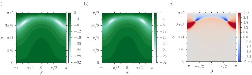
In this section we use the angle definitions indicated in fig.1a, allowing the incident wave to enter the boundary layer at a cross-flow angle (nonzeroβ). In fig.4results for case A at Re = 4×105_are

plotted, where the colour bar scale is in decibels. Figures4a,5aand5bshow the viscous models, while figs. 4b and 6a–6c show the inviscid models. At steep angles of incidence (α .π/8) the viscous and inviscid results vary only slightly, as in the 2D case. At shallower angles, the features of the viscous and inviscid density plots start to change, with greater attenuation occurring in the viscous case in the upstream direction (asβ approaches π or −π). This is seen more easily in fig.4c, which shows the error, in decibels, of the inviscid LEE numerics (fig.4b) with respect to the viscous LNSE numerics (fig.4a). Large regions in (α, β) space show discrepancies of more than 3 dB between the inviscid and viscous attenuation predictions, with a maximum error being an under-prediction of∼17 dB by the inviscid numerics for upstream propagating incident waves entering the boundary layer at shallow angles.

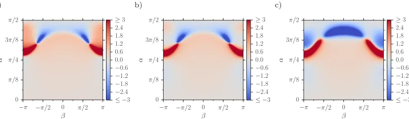
The features of the viscous LNSE numerics, shown in fig. 4a, are captured well by the two viscous asymptotic models, figs.5aand5b. The second-order inviscid boundary condition, fig.6a, performs well in 3D, accurately reproducing the features of the inviscid LEE numerics, fig. 4b, although since this is still inviscid it shows the same inaccuracies as the LEE when compared with the LNSE solution. The Myers and ASP conditions, figs.5cand6c, fail to capture the complicated changes in reflection coefficient that occur asβ is varied for shallow entry angles (α&3π/8).

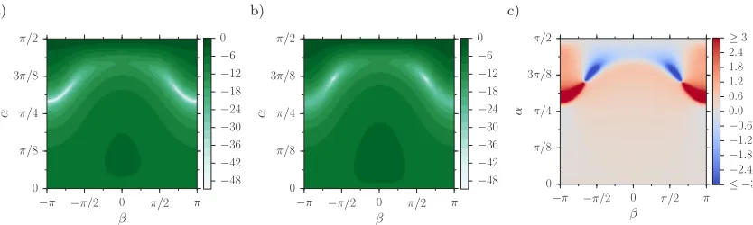
More substantial differences between the viscous and inviscid attenuation predictions can be seen in fig.7, which shows results for case E at Re = 1×105_{. The inclusion of viscosity creates}

patches of very intense attenuation, leading to a maximum under-prediction by the inviscid nu-merics of 32 dB. It is also worth noting the change in polarity of the discrepancy between the LNSE and LEE numerics as the direction of propagation varies between upstream propagating and cross-flow propagating (see fig. 7c). Neglecting viscosity leads to an under-prediction of at-tenuation nearβ=±πwhere the wave is propagating almost directly upstream, but this switches to an over-prediction for −5π/8 . β . 5π/8 where the wave is propagating either across the mean flow or downstream. Again, the asymptotic boundary conditions perform well, capturing the complexities of the attenuation patterns of the numerics in (α, β) space.

IV

Conclusion

By calculating the reflection coefficient for a plane acoustic wave reflecting from an impedance lining in sheared viscous flow, we have investigated the effects of both shear and viscosity on the performance of acoustic linings. For the cases considered, intended to be realistic of a modern turbofan aeroengine (with Re ≈ 105_–107_{), viscosity was found to have an effect on the sound}

a)

−π −π/2 0 π/2 π

β 0

π/8

π/4 3π/8

π/2

α

≤ −3

−2.4

−1.8

−1.2

−0.6 0.0 0.6 1.2 1.8 2.4

≥3 b)

−π −π/2 0 π/2 π

β 0

π/8

π/4 3π/8

π/2

α

≤ −3

−2.4

−1.8

−1.2

−0.6 0.0 0.6 1.2 1.8 2.4

≥3 c)

−π −π/2 0 π/2 π

β 0

π/8

π/4 3π/8

π/2

α

≤ −3

−2.4

−1.8

−1.2

−0.6 0.0 0.6 1.2 1.8 2.4

≥3

Figure 5: Error in the reflection coefficient in decibels, 20 log10|R|/|RLN SE|, for case A from table1

for the viscous boundary conditions: (a) high frequency (Khamis and Brambley, 2017), (b) two deck (Khamis and Brambley,2016b), (c) low Mach number (Aur´egan et al.,2001). The Reynolds number is Re = 4×105_.

a)

−π −π/2 0 π/2 π

β 0

π/8

π/4 3π/8

π/2

α

≤ −3

−2.4

−1.8

−1.2

−0.6 0.0 0.6 1.2 1.8 2.4

≥3 b)

−π −π/2 0 π/2 π

β 0

π/8

π/4 3π/8

π/2

α

≤ −3

−2.4

−1.8

−1.2

−0.6 0.0 0.6 1.2 1.8 2.4

≥3 c)

−π −π/2 0 π/2 π

β 0

π/8

π/4 3π/8

π/2

α

≤ −3

−2.4

−1.8

−1.2

−0.6 0.0 0.6 1.2 1.8 2.4

≥3

Figure 6: Error in the reflection coefficient in decibels, 20 log10|R|/|RLN SE|, for case A from table1

for the inviscid boundary conditions: (a) second order (Khamis and Brambley, 2016a), (b) first order (Brambley,2011), (c) leading order (the Ingard–Myers condition,Ingard,1959,Myers,1980).

a)

−π −π/2 0 π/2 π

β 0 π/8 π/4 3π/8 π/2 α −48 −42 −36 −30 −24 −18 −12 −6 0 b)

−π −π/2 0 π/2 π

β 0 π/8 π/4 3π/8 π/2 α −48 −42 −36 −30 −24 −18 −12 −6 0 c)

−π −π/2 0 π/2 π

β 0

π/8

π/4 3π/8

π/2

α

≤ −3

−2.4

−1.8

−1.2

−0.6 0.0 0.6 1.2 1.8 2.4

≥3

Figure 7: As in fig.4but for case E from with a Reynolds number of Re = 1×105_{. The maximum}

a)

−π −π/2 0 π/2 π

β 0

π/8

π/4 3π/8

π/2

α

≤ −3

−2.4

−1.8

−1.2

−0.6 0.0 0.6 1.2 1.8 2.4

≥3 b)

−π −π/2 0 π/2 π

β 0

π/8

π/4 3π/8

π/2

α

≤ −3

−2.4

−1.8

−1.2

−0.6 0.0 0.6 1.2 1.8 2.4

≥3 c)

−π −π/2 0 π/2 π

β 0

π/8

π/4 3π/8

π/2

α

≤ −3

−2.4

−1.8

−1.2

−0.6 0.0 0.6 1.2 1.8 2.4

≥3

Figure 8: As in fig.5but for case E from table1for a Reynolds number of Re = 1×105_.

a)

−π −π/2 0 π/2 π

β 0

π/8

π/4 3π/8

π/2

α

≤ −3

−2.4

−1.8

−1.2

−0.6 0.0 0.6 1.2 1.8 2.4

≥3 b)

−π −π/2 0 π/2 π

β 0

π/8

π/4 3π/8

π/2

α

≤ −3

−2.4

−1.8

−1.2

−0.6 0.0 0.6 1.2 1.8 2.4

≥3 c)

−π −π/2 0 π/2 π

β 0

π/8

π/4 3π/8

π/2

α

≤ −3

−2.4

−1.8

−1.2

−0.6 0.0 0.6 1.2 1.8 2.4

≥3

Figure 9: As in fig.6but for case E from table1.

Viscosity was found to have a greater effect for upstream and cross-stream propagating waves, and less of an effect for waves with normal incidence or waves predominantly propagating down-stream. Interestingly, neglecting viscosity was found to lead to an underprediction in the atten-uation for upstream propagating waves, and to an overprediction in attenatten-uation for cross-stream propagating waves. This variation could be important for spinning rotor-alone tones in aeroengine intakes or for sound attenuation in swirling mean flows, as both involve both an upstream and a cross-stream component.

The Myers boundary condition was found to be unsuitable for predicting attenuation, with errors of the order of 10 dB, confirming the conclusion ofGabard (2013), as was the low-Mach-number viscous boundary condition ofAur´egan et al.(2001). The first order inviscid generalization of the Myers boundary condition (Brambley, 2011) was found to closely approximate the full linearized Euler equations, while the second order inviscid generalization (Khamis and Brambley,

2016a) results were in almost all cases indistinguishable from those of the linearized Euler equations. Of the two viscous approximate boundary conditions considered, the high-frequency boundary condition (Khamis and Brambley, 2017) performed the best for the cases considered here, and was impressively close (usually within 1 dB) to the results for the full linearized Navier–Stokes equations. The accuracy of this boundary condition may be due to the high frequencies con-sidered, but since these frequencies are typical of aeroengines, this boundary condition could be expected to give accurate results in aeroacoustic applications. The two-deck boundary condi-tion (Khamis and Brambley, 2016b), while not quite as accurate as the high-frequency boundary condition, is still more accurate than any of the inviscid boundary conditions (e.g. fig.3b), includ-ing the full linearized Euler equations.

Acknowledgements

References

C. S. Allen, T. J. Mueller, W. K. Blake, R. P. Dougherty, D. Lynch, P. T. Soderman, and J. R. Underbrink.Aeroacoustic Measurements, chapter 1, pages 34–40. Experimental Fluid Mechanics. Springer, 2013. ISBN 9783662050583.

Y. Aur´egan, R. Starobinski, and V. Pagneux. Influence of grazing flow and dissipation effects on the acoustic boundary conditions at a lined wall. J. Acoust. Soc. Am., 109:59–64, 2001. doi: 10.1121/1.1331678.

G. Boyer, E. Piot, and J.-P. Brazier. Theoretical investigation of hydrodynamic surface mode in a lined duct with sheared flow and comparison with experiment.J. Sound Vib., 330:1793–1809, 2011. doi: 10.1016/j.jsv.2010.10.035.

E. J. Brambley. A well-posed boundary condition for acoustic liners in straight ducts with flow.

AIAA J., 49(6):1272–1282, 2011. doi: 10.2514/1.J050723.

M. O. Burak, M. Billson, L.-E. Eriksson, and S. Baralon. Validation of a time- and frequency-domain grazing flow acoustic liner model.AIAA J., 47(8):1841–1848, 2009. doi: 10.2514/1.40870. M. S. Cramer. Numerical estimates for the bulk viscosity of ideal gases.Phys. Fluids, 24(6), 2012.

doi: 10.1063/1.4729611.

G. Gabard. A comparison of impedance boundary conditions for flow acoustics. J. Sound Vib., 332:714–724, 2013. doi: 10.1016/j.jsv.2012.10.014.

U. Ingard. Influence of fluid motion past a plane boundary on sound reflection, absorption, and transmission. J. Acoust. Soc. Am., 31:1035–1036, 1959. doi: 10.1121/1.1907805.

D. Khamis and E. J. Brambley. Acoustic boundary conditions at an impedance lining in inviscid shear flow. J. Fluid Mech., 796:386–416, 2016a. doi: 10.1017/jfm.2016.273.

D. Khamis and E. J. Brambley. Analytic model and concise impedance boundary condition for viscous acoustics in ducted shear fow. AIAA paper 2016-2976, 2016b.

D. Khamis and E. J. Brambley. Viscous effects on the acoustics and stability of a shear layer over an impedance wall. J. Fluid Mech., 810:489–534, 2017. doi: 10.1017/jfm.2016.737.

D. Marx and Y. Aur´egan. Effect of turbulent eddy viscosity on the unstable surface mode above an acoustic liner. J. Sound Vib., 332:3803–3820, 2013. doi: 10.1016/j.jsv.2013.02.005.

D. Marx, Y. Aur´egan, H. Bailliet, and J.-C. Vali`ere. PIV and LDV evidence of hydrodynamic instability over a liner in a duct with flow. J. Sound Vib., 329:3798–3812, 2010. doi: 10.1016/j. jsv.2010.03.025.

M. K. Myers. On the acoustic boundary condition in the presence of flow. J. Sound Vib., 71: 429–434, 1980. doi: 10.1016/0022-460X(80)90424-1.

D. C. Pridmore-Brown. Sound propagation in a fluid flowing through an attenuating duct.J. Fluid Mech., 4:393–406, 1958. doi: 10.1017/S0022112058000537.

Y. Renou and Y. Aur´egan. Failure of the Ingard–Myers boundary condition for a lined duct: An experimental investigation. J. Acoust. Soc. Am., 130:52–60, 2011. doi: 10.1121/1.3586789. S. W. Rienstra and M. Darau. Boundary-layer thickness effects of the hydrodynamic instability

along an impedance wall. J. Fluid Mech., 671:559–573, 2011. doi: 10.1017/S0022112010006051. G. G. Stokes. On the theories of the internal friction in fluids in motion, and of the equilibrium