Computational Analysis for Predicting Scouring Around Cuboid Shaped Pier in a Stream

(1)

Computational Analysis for Predicting

Scouring Around Cuboid Shaped Pier in a

Stream

Dhruv Saxena

1

1_{M.E. Student, M.B.M. Engineering, JNV University Jodhpur, Rajasthan, India}

Abstract —Scour around bridge piers as a result of

flooding is the most common cause of bridge failure (Richardson and Davis, 1995; Johnson and Dock, 1996; Lagasse et. al., 1995; Melville and Hadfield, 1999). The bridge failures result in excessive repairs, loss of accessibility, or even death (Chiew, 1995). The potential cost including human toll and monetary cost of bridge failure due to scour damage has highlighted the need for better scour prediction and protection methods. A large depth of foundation is required for bridge piers to overcome the effect of scour which is a costly proportion. Therefore, for safe and economical design, scour around the bridge piers is required to be controlled. In this article we have analysed various vulnerable zones formed due to the flow of water in channel.

Keywords — scouring, computational, ANSYS, CAD, CATIA, FLUENT, ICEM, pier, stream, erosion, river bed.

I. INTRODUCTION

Scour is defined as the erosion of streambed around an obstruction in a flow field (Chang, 1988). The amount of reduction in the streambed level below the bed level of the river prior to the commencement of scour is referred as the scour depth. A scour hole is defined as depression left behind when sediment is washed away from the riverbed in the vicinity of the structure. Local scour refers to the removal of sediment from the immediate vicinity of bridge piers or abutments. It occurs due to the interference of pier or abutment with the flow, which results in an acceleration of flow, creating vortices that remove the sediment material in the immediate surroundings of the bridge pier or abutment.

The local scour has the potential to threaten the structural integrity of bridge piers, ultimately causing failure when the foundation of the pier is undermined. Besides the human loss, bridge failures cost crores of rupees in direct expenditure for replacement and restoration in addition to the indirect expenditure related to the disruption of transportation facilities.

The purpose for undertaking this study was to show the most vulnerable zones in the river bed which are created by obstruction to the flow of water created by the pier. These zones are the most

common sites of scouring. To study about this a computer model has been created with the help of CATIA and FLUENT modelling software and used a cuboidal object resembling to a cuboidal pier.

II. GENERAL SOIL CHARACTERISTICS OF RIVER

BED IN INDIA

Major Soil types in India include namely – Red Soils, Laterite Soils, Black Soils, Alluvial Soils, Desert Sand etc., but the most abundant of all in river system is Alluvial Soil. Alluvial soils are scattered throughout the country and is the most widespread category. These soils cover 40% of the entire land area in India.

The river deposits extremely refined particles of soil, called alluvium in their plains during the path of their long travel, spread over hundreds of kilometres and thousands of years.

The river beds consist of soils of varying particle sizes. It contains finest clay to coarse sand along its flow. Different particles have different setting velocities as we know and turbulence also affects them varyingly.

III.PROTECTION OF SCOURING AROUND BRIDGE

PIERS

Scour around bridge piers as a result of flooding is the most common cause of bridge failure (Richardson and Davis, 1995; Johnson and Dock, 1996; Lagasse et. al., 1995; Melville and Hadfield, 1999). The bridge failures result in excessive repairs, loss of accessibility, or even death (Chiew, 1995). The potential cost including human toll and monetary cost of bridge failure due to scour damage has highlighted the need for better scour prediction and protection methods.

A large depth of foundation is required for bridge piers to overcome the effect of scour which is a costly proportion. Therefore, for safe and economical design, scour around the bridge piers is required to be controlled.

(2)

riprap around the pier (Brice et. al., 1978; Croad, 1993; Parola,1993; Yoon et. al., 1995; Worman 1989, (Lim and Chiew, 1996 and 1997); Lim, 1998; Chiew and Lim, 2000; Lim and Chiew, 2001), providing an array of piles in front of the pier (Chabert and Engeldinger, 1956 and Melville and Hadfield,1999), a collar around the pier (Schneible, 1951; Thomas 1967; Tanaka and Yano 1967; Ettema 1980; Chiew, 1992; kumar et. al., 1999, Zarrati et. al., 2004, Zarrati et. al., 2006), submerged vanes (Odgard and Wang 1987), a delta-wing-like fin in front of the pier (Gupta and Gangadharaiah, 1992), a slot through the pier (Chiew, 1992; Kumar et. al., 1999) and partial pier-groups (Vittal et. al., 1994) and tetrahedron frames placed around the pier.

IV.REASONS FOR SCOURING

Scour of the riverbeds around bridge supports is the most frequent cause of their failures. Maintenance and repair costs of the bridges damaged by scour effects are significant, but it is estimated that the social costs are five times higher than the direct repair and replacement costs. The condition for the proper monitoring of scour is to understand its nature. The knowledge of the phenomena occurring during the high water flow in the area of the bridge supports is crucial to properly assess the current condition and to develop proper maintenance actions.

Scour may be the consequence of:

• Narrowing the watercourse – a natural or man-made, including construction of a bridge.

• Lateral movement or lowering of the stream bed.

• Hydraulic works shortening the length of the meandering section of the watercourse.

• Changes occurring in the catchment area of the watercourse.

• Other changes in watercourse hydrology. The presence of a bridge causes the stream flow cross-section reduction, which increases the speed and intensity of erosion of the streambed. River tends to stabilize its bed in order to restore the natural flow section. Bridge supports also change the laminar water flow and turbulent flow.

V. GENERAL SCOUR AND LOCAL SCOUR

Scour is defined as the erosion of streambed around an obstruction in a flow field (Chang, 1988). The amount of reduction in the streambed level below the bed level of the river prior to the commencement of scour is referred as the scour depth.

General scour is defined as the general lowering of the sediment bed that can occur during the passage of a flood wave. Scour–removal by hydrodynamic forces of granular bed material in the vicinity of structures place on coastal areas or river basins. Scour is a specific form of the more general term erosion.

Local scour around a bridge pier will begin when the downflow velocity near the stagnation point becomes strong enough to overcome resistance forces of the bed particles. Once these forces are exceeded, particles will be dislodged and carried downstream by the horseshoe vortex and/or the wake vortex.

VI.LITERATURE FOR OPEN CHANNEL FLOW,

LAMINAR FLOW AND TURBULENT FLOW

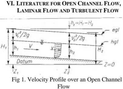
Fig 1. Velocity Profile over an Open Channel Flow

Open Channel Flow -- It is a type of liquid flow within a conduit with a free surface, known as a channel. This means that the pressure acting on the top surface of the flow is atmospheric pressure unlike pipe flow where the pressure is usually higher than the atmospheric pressure, in a pipe flow the water flows due to this pressure gradient while in the open channel flow (flow in canals, rivers) the flow occurs due to the gradient slope of the channel bed.

Laminar Flow -- Laminar flow is the type of low in which the streamlines are parallel to each other and do no intersect each other’s path. Flow in which the kinetic energy dies out due to the action of fluid molecular viscosity is called laminar flow.

Turbulent Flow -- It is the flow condition in which the streamlines crisscross each other and are not parallel as in instance of laminar flow. Turbulent flows are at all times highly irregular. To sustain turbulent flow, a persistent support of energy supply is required because turbulence disperses rapidly as the kinetic energy is transformed into internal energy by viscous shear stress.in turbulent flow water mixes from one layer to other layer.

Boundary Layer -- A boundary layer is the layer of fluid in the immediate vicinity of a bounding surface where the effects of viscosity are significant. The boundary layer grows from zero when a fluid starts to flow over a solid surface. As it passes over a greater length more fluid is slowed by friction between the fluid layers close to the boundary. Hence the thickness of the slower layer increases.

VII. SOFTWARE USED AND MODELLING

METHOD

(3)

dimensions. The working principles are discussed in later sections.

2. ICEM CFD (ANSYS) – CFD stands for Computational Fluid Dynamics. ANSYS ICEM CFD meshing software starts with cutting-edge CAD/geometry readers and repair gears to allow the user to speedily progress to a diversity of geometry-tolerant mesh and yield high-quality volume or surface meshes with nominal effort.

3. FLUENT 14.0 - ANSYS Fluent software comprises the broad physical modeling capabilities required to model flow, turbulence, heat transfer, and reactions for industrial applications ranging from air flow to dynamic fluid flow.

Geometric Modelling – The geometric modelling structures are prominently used as to ―clean-up‖ an imported CAD file. ANSYS ICEM CFD is used here to mesh the required geometry. There are many similar packages available which perform similarly. ANSYS ICEM CFD provides many editing and repairing tools which are both manual as well as automatic that aid in arriving at the meshing stage rapidly.

Meshing Approach - ANSYS ICEM CFD provides advanced geometry acquisition, mesh generation and mesh optimization tools to meet the requirement for integrated mesh generation for today’s sophisticated analysis. ICEM CFD is used especially in engineering applications such as computational fluid dynamics and structural analysis.

As we mentioned earlier also, that ICEM CFD provides a direct link between geometry and analysis. Geometry can be input from any CAD design package. ICEM CFD’s open geometry database offers flexibility to combine geometric information in various forms of mesh generation.

ANSYS FLUENT 14.0 - ANSYS FLUENT offers an unparalleled breadth of turbulence models including several versions of the time-honoured k-epsilon and k-omega models, as well as the Reynolds stress model (RSM) for highly swirling or anisotropic flows. ANSYS FLUENT offers an unparalleled breadth of turbulence models including several versions of the time-honoured k-epsilon and k-omega models, as well as the Reynolds stress model (RSM) for highly swirling or anisotropic

flows.

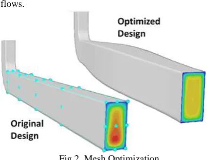
Fig 2. Mesh Optimization

ANSYS FLUENT provides complete mesh flexibility, including the ability to solve orr flow problems using unstructured meshes that can be generated about complex geometries with relative ease. Supported mesh types include triangular, quadrilateral, tetrahedral, hexahedral, pyramid, prism (wedge), and polyhedral meshes.

The basic procedural steps for solving a problem in FLUENT include:

1. Define the modelling goals.

2. Create the model geometry and grid. 3. Set up the solver and physical models. 4. Compute and monitor the solution. 5. Examine and save the results.

6. Consider revisions to the numerical or physical model parameters, if necessary FLUENT can model flow involving moving reference frames and moving cell zones, using several different approaches, and flow in moving and deforming domains (dynamic meshes).

VIII. CALCULATIONS

As we mentioned earlier also, that ICEM CFD provides a direct link between geometry and analysis. Geometry can be input from any CAD design package. ICEM CFD’s open geometry database offers flexibility to combine geometric information in various forms of mesh generation.

(4)

Fig 3. Work Flow Chart

Checking the Mesh

The mesh editing tools in ANSYS ICEM CFD allow us to diagnose and fix problems in the mesh. A number of manual and automatic tools are available for operations such as conversion of element types, refining or coarsening the mesh, smoothing the mesh, etc. The process involves the following:

1. Check the mesh for problems such as holes, gaps, overlapping elements using the diagnostic checks available. Fix the problems using the appropriate automatic or manual repair methods. 2. Check the elements for bad quality and use

smoothing to improve the mesh quality.

3. If the mesh quality is poor, it may be appropriate to fix the geometry instead or recreate the mesh using more appropriate size parameters or a different meshing method.

Generating Input for the Solver

ANSYS ICEM CFD includes output interfaces to various flow and structural solvers, producing appropriately formatted files that contain complete mesh and boundary condition information. After selecting Fluent as solver, we can modify the solver parameters and write the necessary input files. The output interfaces option opens the information about specific interface, refer to the Table of Supported solvers and click the name of the interface. The GUI is easy to use with mostly used tools as icons in different toolbars.

Fluent Solver

From the tetra mesh geometry achieved from ICEM CFD, we use the pressure based solver technique of Fluent 14.0. The pressure-based solver conventionally has been used for incompressible and mildly compressible flows. The density-based approach, on the other hand, was initially designed for high-speed compressible flows. Both methodologies are now relevant to a broad collection of flows (from incompressible to highly compressible).

When selecting a solver and an algorithm we must consider the following issues:

1. The model readiness for a given solver.

2. Solver efficiency for the given flow conditions.

3. The size of the mesh under concern and the accessible memory on our machine.

Fig 4. User Interface of ICEM CFD Reference: ANSYS Online Internet Help

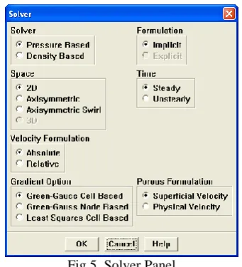
Inputs for Solver Selection - To pick one of the solver interpretations, we will use the solver panel:

Fig 5. Solver Panel

After we have demarcated our model and quantified which solver we want to use, we are ready to execute the solver. The following steps outline a brief procedure we have followed:

1. Select the discretization scheme and, for the pressure-based solver, the pressure interpolation scheme.

(5)

4. Select how we want the derivatives to be evaluated by choosing a gradient alternative.

5. Set the under-relaxation factors. 6. Turn on FAS multi-grid.

7. Make any further modifications to the solver settings that are proposed in the chapters or sections that define the models we are using.

8. Initialize the solution.

9. Permit the appropriate solution monitors. 10. Start calculating for steady-state calculations, time-dependent calculations.

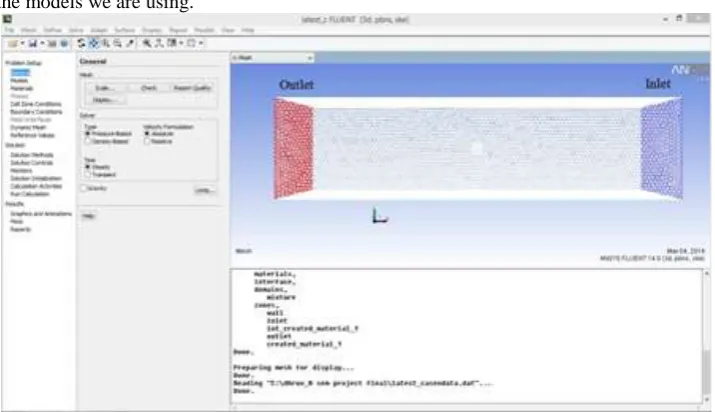
Fig 6. Screenshot of Tetra Mesh Channel to be used in ANSYS FLUENT.

Fig 7. Geometric Front View of Channel Fig 8. Geometric Top View of Channel

Monitoring Solution Convergence - During the solution process we can observe the convergence dynamically by checking residuals, statistics, force values, surface integrals, and volume integrals. We can print results of or display plots of lift, drag, and moment coefficients, surface integrations, and residuals for the solution variables. For unsteady flows, we can also observe lapsed time.

Controlling Normalization – By default, scaling of residuals is enabled and the default convergence criterion is 10-6 for energy and P-1 equations & 10

-3_{for all other equations. Residual normalization (i.e.,}

dividing the residuals by the largest value during the first few iterations) is also available but disabled by default.

Judging Convergence - There are no universal metrics for judging convergence. Residual definitions that are useful for one class of problem are sometimes misleading for other classes of problems. Therefore it is a good idea to judge convergence not only by examining residual levels, but also by monitoring relevant integrated quantities

such as drag or heat transfer coefficient. For most problems, the default convergence criterion in FLUENT is sufficient.

Parameters entered for Analysis –

1. Scale – in meters 2. Solver – Pressure based

3. Velocity Formulation – Absolute 4. Time – Steady

5. Material Properties – Water as fluid in Metal channel.

6. Boundary Conditions – Definitions for wall, inlet, outlet and internally created material (pier).

Solution Methods

1. Gradient – Least squares cell based. 2. Pressure – Standard.

3. Momentum, Turbulent Kinetic Energy – Default.

(6)

3. Body Forces - 1 4. Momentum – 0.7 5. Kinetic Energy – 0.8

Monitors

1. Mass Flow vs Iteration count.

Script for initializing the solver calculations: 417779 tetrahedral cells, zone 15, binary. 822130 triangular interior faces, zone 16, binary. 1384 triangular velocity-inlet faces, zone 17, binary. 1458 triangular pressure-outlet faces, zone 18, binary.

24014 triangular wall faces, zone 19, binary. 76485 nodes, binary.

76485 node flags, binary. Building...

mesh materials, interface, domains, mixture zones, wall

inlet

int_created_material_1 outlet

created_material_1 Done.

Now, we start the Hybrid Initialization for running the calculations, we get following iteration values:

Initialize using the hybrid initialization method. Checking case topology.

-this case has inlets & outlets both

-pressure information is not available at the boundaries,

So, it will be initialized with constant pressure iter scalar-0

1 1.000000e+00

2 6.196463e-04

3 1.041858e-04

4 3.816625e-05

5 9.699194e-06

6 3.200364e-06

7 9.847464e-07

8 3.432748e-07

9 1.308455e-07

10 5.778368e-08

After, the above hybrid initialization is completed, we run the calculations by taking a total of 500 iteration processes with an interval reporting at each step.

Data Found from iterations –

Iteration continuity x-velocity y-velocity z-velocity k epsilon surf-mon-1 time/iteration turbulent viscosity limited to viscosity ratio of 1.000000e+05 in 162 cells

1. 1.0000e+00 1.7608e-03 1.7564e-03 1.6936e-03 1.3174e-02 1.7147e-01 -1.0005e+05 0:24:57 499 turbulent viscosity limited to viscosity ratio of 1.000000e+05 in 97 cells

2. 4.4286e-01 6.3602e-04 5.3074e-04 4.7712e-04 1.2367e-02 4.1401e-02 -9.9892e+04 0:24:54 498 turbulent viscosity limited to viscosity ratio of 1.000000e+05 in 189 cells

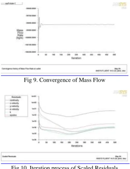
Similarly, we continue the iterative process until we observe the difference in consecutive iterations of scaled residuals of k – epsilon, velocity and continuity equation below 1e-06. Another condition of a continuous flow should be achieved in the channel flow. Hence, we continue the iterative processes up to 500 times.

Following graphs show the Iteration process data graphs for scaled residuals and convergence history of mass flow from Fluent solver 14.

Fig 9. Convergence of Mass Flow

Fig 10. Iteration process of Scaled Residuals

(7)

Fig 11. Graphic animation of Channel from Fluent.

IX.PLOTS FOR MAJOR VULNERABLE ZONES

Fluent 14.0 solver helps in calculations and analysis of various parameters of Fluid Dynamics. Upon complete iterations, we obtain plots of depicting Vector diagrams and Contours of various parameters like, pressure, density, velocity (tangential and radial), turbulence kinetic energy. For analysing in various perspectives for better results we have opted 12 planes consisting of 3 horizontal planes with normal to bed and 10 planes vertically aligned depicting various parameters.

These plots will show us the major zones where turbulence forces may be observed and also possible erosion zones around a cuboidal bridge pier. Here we have used a scale model and presented the following parameters – Total Pressure, Turbulent Intensity, Vorticity Magnitude, Turbulent Kinetic Energy.

Plots obtained on Horizontal Planes

1. Plane at 0.001m above channel bed –

Fig 12. Velocity Vectors Colored by Total Pressure (pascal)

Fig 13. Velocity Vectors Colored by Turbulent Intensity (%)

Fig 14. Velocity Vectors Colored by Vorticity Magnitude (1/s)

Fig 15. Velocity Vectors Colored by Turbulent Kinetic Energy (k) (m2/s2)

Fig 16. Contours of Total Pressure (pascal)

Fig 17. Contours of Turbulent Intensity (%)

Fig 18. Contours of Vorticity Magnitude (1/s)

(8)

2. Plots obtained at Mid-section (1m above bed)

Fig 21. Velocity Vectors Colored by Turbulent Intensity

Fig 22. Velocity Vectors Colored by Turbulent Kinetic Energy

Fig 23. Velocity Vectors Colored by Vorticity Magnitude (m/s)

Fig 27. Contours of Turbulent Kinetic Energy (k) (m2/s2)

3. Plots obtained for Top Boundary Layer (1.999m above channel bed)

Fig 29. Velocity Vectors Colored by Vorticity Magnitude (1/s)

Fig 30. Velocity Vectors Colored by Turbulent Kinetic Energy (k)(m2/s2)

(9)

Fig 35. Contours of Turbulent Kinetic Energy (k)(m2/s2)

Plots obtained on Vertical Planes (longitudinal) 1. Plots obtained on Mid Section

2. Plots obtained on Boundary Layer (Inlet Side)

(10)

3. Plots obtained on Boundary Layer (Outlet Side)

Plots Obtained on Vertical Planes (along Cross Section)

1. Plots obtained at Mid-Section

X. CONCLUSION

The paper dealt with analysis of bridge pier over a flowing river and effects of water over the river bed soil. Various researchers have done research on circular pier, in this article the study of was done about cuboidal pier for bridges, the various major zones where we might observe soil erosion. In this paper, a scale model was used to simulate a pier using ANSYS FLUENT 14.0. The analysis was carried by constructing a geometry model with the help of CATIA followed by Tetra mesh construction of volume materials with the use of ANSYS ICEM CFD (Computational Fluid Dynamics). The model assumed was based on the contraction theories.

Analysis was carried by Pressure base solver method in Fluent with 500 iterations for convergence of mass flow till the flow was relatively stable. Plots and animations for Vector and Contours of various fluid mechanics parameters. These plots provide a basic idea about the various flow characteristics around the Pier which provides a basic idea about the designing of pier and also what modifications to be made to the river bed to maintain safe conditions.

With the consideration of a rectangular channel, by obtaining pressure and velocity variations, we analysed the regions highly prone to scouring with static as well as dynamic parameters obtained. The results also show the Vortex formed during the fluid flow, pressure and density variations which effect the stability of pier.

(11)

and cementing or grouting of river bed zones prone to erosion due to turbulence of flowing river wherever required.

XI.REFERENCES

1. Ahmed, F., and Rajaratnam N.. Flow around Bridge Piers, Am. Soc. Civ. Engrg., J. Hydr. Engrg, 1998, 124(3), 288-300. 2. Ansys online user guides.

3. Baker, C. J. ―New Design Equations for scour around bridge

piers‖, ASCE Journal of the Hydraulics Division.

4. Bonasoundas, Dr. Ing.. Flow structure and scour problem at

circular bridge piers, 1973, Report No; 28, Oskar Von,

Miller Institute, Munich Technical University.

5. Brice, J. C., Bloggett, J.C. and others.Countermeasures for

Hydraulic Problems at Bridge Piers, 1978, Vol. 1 and

2,FHWA-78-162 & 163, 1978, Federal Highway Administration, U.S. Department of transportation, Washington, D.C.

6. Breusers, H.N.C., Nicollet, G. and Shen, H.W. Local scour

around cylindrical piers, J. Hydr. Res., Delft, The

Netherlands, 1977,15(3), pp. 211-252. 7. Catia online user guides.

8. Chabert, J. and Engeldinger, P.. Etude des affouillement

autour des Piles des ponts (Study on Scour around bridge

piers), Laboratoire National d’Hydraulique, Chatou, 1956, France.

9. Chang, F.F.M., (1980) ―Scour at Bridge Piers – Field Data

from Loisian Files‖, Washington.

10. Chang, H.H.. Fluvial processes in river engineering, John Wiley & Sons, 1998, 432p.

11. Chiew Y.M. “Mechanics of Riprap Failure at Bridge Piers‖, J. of Hydraulic Engineering, ASCE, Vol. 121, No. 9, 1995, pp. 635-643.

12. Chiew, Y.M. Scour Protection at Bridge Piers, J. Hydr. Engrg., ASCE, 1992, 118(9), 1260-1269.

13. Chiew Y.M. and Lim, F. H. ―Failure Behavior of Riprap

Layer at Bridge Piers under Live-Bed Conditions‖, J. Hydr.

Engrg, ASCE, 2000, 126(1), 43-55.

14. Croad, R.N. Bridge Pier Scour Protection Using Riprap, Central Laboratories Report No. PR3-0071, 1993, Works Consultancy Services, N.Z.

15. Dargahi, B., Controlling Mechanism of Local Scouring, J. Hydr. Engrg, ASCE, 1990, 116(10), 1197-1214.

16. Dey, S. Local Scour at Piers, part I: A Review of

Developments of Research, IRTCES, Int. J. Sediment Res.,

1997, 12(2), 23-44.

17. Ettema, R. ―Scour at Bridge Piers‖, 1980, Report No. 216, School of Engrg., University of Auckland, Auckland, New Zeeland.

18. Elliott K.R., and Baker, C.J., (1985) ―Effect of pier spacing

on scour around bridge piers‖, ASCE Journal of Hydraulic

Engineering.

19. Garde, R.J. and Kothyari, U.C., State of art report on scour

around bridge piers, 1995, Pune, India.

20. Grade, R.J., (1961) ―Local Bed Variation at Bridge Piers in

Alluvial Channels‖, University of Roorkee Research Journal.

21. Graf, W.H. and Istiarto, Flow Pattern in the Scour Hole

around a Cylinder, Journal of Hydraulic Research, 2002,Vol.

40, No. 1, pp. 13-20.

22. Gupta, A.K. and Gangadharaiah, T. Local scour reduction by a delta wing-lick passive device, 1992, Proc., 8th Congr. of Asia and Pacific Reg. Div., 2, CWPRS, Pune, India, pp. B471-B481.

23. Hadfield, A.C. Sacrificial piles as a bridge pier scour counter-measure, 1997, ME thesis, Civ. and Resour. Engrg. Dept., University of Auckland, Auckland, New Zealand.

24. Hager, W. H. and Oliveto, G. Shields’ entrainment criterion in bridge hydraulics, journal of hydraulic engineering, ASCE, 2002, 128 (5), pp. 538-542.

25. Haghighat, M. Scour around bridge pier group, 1993, ME thesis, University of Roorkee, Roorkee, India.

26. HEC-18. Evaluating scour at bridges, Hydraulic Engineering Circular No. 18, 1991, Federal Highway Administration (FHWA), USDOT, Washington, D.C.

27. Hjorth, P. Study on the Nature of Local Scour, 1975, Department of Water Resources, Lund Inst. of Tech., Lund, Sweden, Bulletin Series A, No. 46.

28. Hopkins, G.R., Vance, R.W., Kasrae, B.,(1980) ―Scour

Around Bridge Piers‖, Federal Highway Administration,

Washington, DC.

29. Melville, B.W. and Raudkivi, A.J. Flow Characteristics in

Local Scour at Bridge Piers, Am.Soc. Civ. Eng., J. Hydr.

Engrg, 1977, 15(4), 373-380.

30. Neill, C.R., Guide to bridge hydraulics, 1973, Edited by C.R. Neill, published for Roads and Transportation Assn. of Canada by University of Toronto Press.

31. Mubeen B. et. al., (2013) Scour Reduction around Bridge

Piers: A Review, International Journal of Engineering

Inventions, Vol. 2, Issue 7 pp. 07-15.

32. Sarda V.K. (2010) Protection of Bridge Abutments from

Scour, Journal of Indian Water Resources, Vol. 30 No. 1.

33. Shen, H. W., Schneider, V. R. and Karaki, S. S., Mechanics of local scour, data supplement, prepared for bureau of

public roads, 1966, Office of Research and Development,

Civil Engineering Department, Colorado State University,

Fort Collins, CO, Report CER66-67HWS27.

34. Shen, H.W., Schneider, V.R. and Karaki, S., Local scour

around bridge piers, J. of Hydraulic Div., A.S.C.E., 1969,

Vo. 95, No. 6, pp. 1919-1940.