warwick.ac.uk/lib-publications
Original citation:
Bowditch, B. H. and Sakuma, Makoto (2018) The action of the mapping class group on the space of geodesic rays of a punctured hyperbolic surface. Groups, Geometry, and Dynamics, 12 (2). pp. 703-719. doi:10.4171/GGD/453
Permanent WRAP URL:
http://wrap.warwick.ac.uk/97152
Copyright and reuse:
The Warwick Research Archive Portal (WRAP) makes this work by researchers of the University of Warwick available open access under the following conditions. Copyright © and all moral rights to the version of the paper presented here belong to the individual author(s) and/or other copyright owners. To the extent reasonable and practicable the material made available in WRAP has been checked for eligibility before being made available.
Copies of full items can be used for personal research or study, educational, or not-for-profit purposes without prior permission or charge. Provided that the authors, title and full
bibliographic details are credited, a hyperlink and/or URL is given for the original metadata page and the content is not changed in any way.
Publisher’s statement
This article has been accepted for publication in a revised form in the journal Groups, Geometry and Dynamics by publisher EMS Publishing House:
http://www.emsph.org/journals/journal.php?jrn=GGD, DOI: 10.4171/GGD/453. This version is free to view and download for private research and study, non-commercial use only. © European Mathematical Society.
A note on versions:
The version presented here may differ from the published version or, version of record, if you wish to cite this item you are advised to consult the publisher’s version. Please see the ‘permanent WRAP URL’ above for details on accessing the published version and note that access may require a subscription.
SPACE OF GEODESIC RAYS OF A PUNCTURED HYPERBOLIC SURFACE
BRIAN H. BOWDITCH AND MAKOTO SAKUMA
Abstract. Let Σ be a complete finite-area orientable hyperbolic surface with
one cusp, and letRbe the space of complete geodesic rays in Σ emanating from the puncture. Then there is a natural action of the mapping class group of Σ onR. We show that this action is “almost everywhere” wandering.
1. Introduction
Let Σ be a complete finite-area orientable hyperbolic surface with one cusp, and
R the space of complete geodesic rays in Σ emanating from the puncture. Then, there is a natural action of the (full) mapping class group Map(Σ) of Σ onR ≡S1, as we describe in Sections 2 and 3. (Here we are allowing orientation-reversing mapping classes.) The dynamics of the action of an element of Map(Σ) onRplays a key role in the Nielsen-Thurston theory for surface homeomorphisms. It also plays a crucial role in the variation of McShane’s identity for punctured surface bundles with pseudo-Anosov monodromy, established by [Bo1] and [AkMS].
It is natural to ask what does the action of the whole group Map(Σ) (or its subgroups) look like. However, the authors could not find a reference which treats this natural question. On the other hand, there are various references which study the action of (subgroups of) the mapping class groups on the projective measured lamination spaces, which are homeomorphic to higher dimensional spheres (see for example, [Mas1, Mas2, MccP, OS]). In particular, such an action is minimal (cf. [FatLP]) and moreover ergodic [Mas1].
The purpose of this paper is to prove that the action of Map(Σ) onRis “almost everywhere” wandering (see Theorem 2.2 for the precise meaning). This forms a sharp contrast to the above result of [Mas1].
While we restrict to the case where Σ has one cusp, we note that one could generalise the statement when there is more than one. However, this would com-plicate the exposition somewhat. (See the remark at the end of Section 6.)
This paper is organised as follows. In section 2, we give a statement of the main result. In Section 3, we give a rigorous construction of the action of Map(Σ) on
Date: 23rd November 2017.
2010Mathematics Subject Classification. 20F65, 20F34, 20F67, 30F60, 57M50 The second author was supported by JSPS Grants-in-Aid 15H03620.
Rby using the theory of the canonical boundary of a relatively hyperbolic group, and then state the main result of this paper. In Section 4, we give an account of the “loop-cutting” construction, and show how it gives rise to a sequence of elements of Γ =π1(Σ), and parabolic points in the boundary of ˜Σ. These “derived sequences” are used in Section 5 to define the concept of a filling point. We show that the set, F, of filling points is an open subset of C whose complement is “small”, in particularF has full measure (Proposition 5.1). In Section 6, we show that the image of F in R is contained in the wandering domain of the action of Map(Σ) on R (Lemma 6.2). The proof of the main result is given by using this result. In Section 7, we give a list of notations used in this paper.
AcknowledgementWe would like to thank Katsuhiko Matsuzaki for his help-ful comments on the first version of the paper. We would also like to thank the referees for their careful reading and valuable suggestions.
2. Statement of main result
Let Σ = H2/Γ be a complete finite-area orientable hyperbolic surface with precisely one cusp, where Γ = π1(Σ). Let R be the space of complete geodesic rays in Σ emanating from the puncture. Then R is identified with a horocycle,
τ, in the cusp. In fact, a point of τ determines a geodesic ray in Σ emanating from the puncture, or more precisely, a bi-infinite geodesic path with its positive end going out the cusp and meeting τ in the given point. Any mapping class ψ
of Σ maps each geodesic ray to another path which can be “straightened out” to another geodesic ray, and hence determines another point ofτ. This gives rise to an action of Map(Σ) on R ≡ τ. This will be discussed more formally in Section 3, where we give a description of the space R as a topological circle constructed independent of a hyperbolic structure of Σ, and then give a rigorous construction of the action of Map(Σ) on R.
In order to state the main result, we prepare some terminology.
Definition. Let G be a group acting by homeomorphism on a topological space
X. An open subset, U ⊆ X, is said to be wandering if gU ∩ U = ∅ for all
g ∈G\ {1}.
Note that this definition is stronger than the usual definition of wandering, where it is only assumed that the number ofg ∈Gsuch that gU∩U 6=∅is finite. The wandering domain, WG(X)⊆ X, is the union of all wandering open sets.
Its complement, Wc
G(X) =X\WG(X), is the non-wandering set.
The following easily verified fact is used in Section 6.
Proposition 2.1. LetH /Gbe a normal subgroup. Then for the induced action of G/H on X/H, we have WG(X)/H ⊆WG/H(X/H) with equality if WH(X) = X.
metrics on R are related by a quasisymmetry. However, they are completely singular with respect to each other (see [K, Tu2]). (That is, there is a set which has zero measure in one structure, but full measure in the other.) In general, this gives little control over how the Hausdorff dimension of a subset can change.
We say that a subset,B ⊆ Ris small if it has Hausdorff dimension stricty less than 1 with respect to any hyperbolic structure on Σ. Now we can state our main theorem.
Theorem 2.2. Let Σbe a once-punctured closed orientable surface, with χ(Σ) <
0, and consider the action of Map(Σ) on the circle R. Then the non-wandering set in R with respect to the action of Map(Σ) is small.
In particular, the non-wandering set has measure 0 with respect to any hyper-bolic structure, and so has empty interior.
Given that two different hyperbolic structures give rise to quasisymmetically related metrics on R, it is natural to ask if there is a more natural way to express this. For example, is there a property of (closed) subsets of R, invariant under quasisymmetry and satisfied by the non-wandering set, which implies Hausdorff dimension less than 1 (or measure 0)?
3. Actions
In this section, we give a more formal account of the action of Map(Σ) on
R ≡τ.
Choose a representative, f, of ψ ∈ Map(Σ), so that its lift ˜f to the universal cover H2 is a quasi-isometry. Then ˜f extends to a self-homeomorphism of the closed disc H2∪∂
H2. For a geodesic rayν ∈ R, let ˜ν be the closure in H2∪∂H2
of a lift of ν to H2. Then ˜f(˜ν) is an arc properly embedded in
H2∪∂H2, and
its endpoints determine a geodesic in H2, which project to another geodesic ray
ν0 ∈ R. Thus, we obtain an action of ψ on R, by setting ψν =ν0. However, one needs to verify that this action does not depend on the choice of a representative
f of ψ.
In the following, we settle this issue, by using the canonical boundary of a relatively hyperbolic group described in [Bo2]. Though we are really interested here only in the case where the group is the fundamental group of a once-punctured closed orientable surface, and the peripheral structure is interpreted in the usual way (as the conjugacy class of the fundamental group of a neighbourhood of the puncture), we give a discussion in a general setting.
Let Γ be a non-elementary relatively hyperbolic group with a given peripheral structure P, which is a conjugacy invariant collection of infinite subgroups of Γ. By [Bo2, Definition 1], Γ admits a properly discontinuous isometric action on a path-metric space,X, with the following properties.
(2) every point of the boundary of X is either a conical limit point or a bounded parabolic point,
(3) the peripheral subgroups, i.e., the elements ofP, are precisely the maximal parabolic subgroups of Γ, and
(4) every peripheral subgroup is finitely generated.
It was proven in [Bo2, Theorem 9.4] that the Gromov boundary ∂X is uniquely determined by (Γ,P), (even though the quasi-isometry class of the space X sat-isfying the above conditions is not uniquely determined). Thus the boundary
∂Γ =∂(Γ,P) is defined to be∂X. By identifying Γ with an orbit inX, we obtain a natural topology on the disjoint union Γ∪∂Γ which is compact Hausdorff, with Γ discrete and∂Γ closed.
The action of Γ on itself by left multiplication extends to an action on Γ∪∂Γ by homeomorphism. This gives us a geometrically finite convergence action of Γ on∂Γ. Let Aut(Γ,P) be the subgroup of the automorphism group, Aut(Γ), of Γ which respects the peripheral structureP. This contains the inner automorphism group, Inn(Γ). Now, by the naturality of ∂Γ ([Bo2, Theorem 9.4]), the action of Aut(Γ,P) on Γ also extends to an action on Γ∪∂Γ, which is Γ-equivariant, i.e.,
φ·(g·x) =φ(g)·(φ·x) for every φ∈Aut(Γ,P), g ∈Γ andx∈Γ∪∂Γ. (In order to avoid confusion, we use · to denote group actions, only in this place.) Under the natural epimorphism Γ −→ Inn(Γ), this gives rise to the same action on ∂Γ as that induced by left multiplication. The centre of Γ is always finite, and for simplicity, we assume it to be trivial. In this case, we can identify Γ with Inn(Γ). Suppose that p ∈ ∂Γ is a parabolic point. Its stabiliser, Z = Z(Γ, p), in Γ is a peripheral subgroup. Now Z acts properly discontinuously cocompactly on ∂Γ\ {p}, so the quotient T = (∂Γ\ {p})/Z is compact Hausdorff (cf. [Bo2, Section 6]). Let A = A(Γ,P, p) be the stabiliser of p in Aut(Γ,P). Then Z is a normal subgroup of A, and we get an action of M = A/Z on T. If there is only one conjugacy class of peripheral subgroups, then the orbit Γp is Aut(Γ,P )-invariant, and it follows that the groupA maps isomorphically onto Out(Γ,P) = Aut(Γ,P)/Inn(Γ), so in this case we can naturally identify the group M with Out(Γ,P).
Suppose now that Σ is a once-punctured closed orientable surface, with negative Euler characteristicχ(Σ). We write Σ =D/Γ, where D= ˜Σ, the universal cover, and Γ ∼= π1(Σ). Let P be the peripheral structure of Γ arising from the cusp of Σ, namely P consists of the conjugacy class of the fundamental group of a neighbourhood of the end of Σ. Then (Γ,P) is a relatively hyperbolic group, because if we fix a complete hyperbolic structure on Σ then D is identified with
H2 and the isometric action of Γ on D = H2 satisfies conditions (1)–(4) in the
above. NowDadmits a natural compactification to a closed disc,D∪C, whereC
is the dynamically defined circle at infinity. We can identifyC with∂Γ. In fact, if
C. If p∈ ∂C is parabolic, then its stabiliser Z in Γ is isomorphic to the infinite cyclic groupZ, and we get an action of Out(Γ,P) on the circleT = (C\ {p})/Z. Since Out(Γ,P) is identified with the (full) mapping class group Map(Σ) of Σ, we obtain a well defined action of Map(Σ) on the circle T.
We now return to the setting in the beginning of this section, where Σ =
H2/Γ is endowed with a complete hyperbolic structure. Then we can identify
the (dynamically defined) circle T with the horocycle, τ, in the cusp, which in turn is identified with the space of geodesic rays, R. This gives an action of Map(Σ) on R. Since the action of Γ on H2 satisfies the conditions (1)–(4) in the above (i.e., [Bo2, Definition 1]), we see that, for each mapping class ψ of Σ, its action on R, defined via the “straightening process” presented at the beginning of this section, is identical with the action which is dynamically constructed in the above, independently from the hyperbolic structure. Thus the problem raised at the beginning of this section is settled.
4. The loop-cutting construction
Let Σ = H2/Γ be a complete finite-area orientable hyperbolic surface with precisely one cusp.
The construction described in this section aims to associate combinatorial data to a ray,ν, emanating from the cusp of Σ. In particular, we will construct a (finite or infinite) sequence of properly embedded arcs, λi, with both endpoints at the
cusp. In Section 6, we will show that if these arcs eventually “fill” Σ, then the ray corresponds to an element of the wandering domain. Since this situation is “generic”, the main result will then follow.
The basic idea behind the construction is as follows. If the ray,ν, is embedded in Σ (properly or not), we immediately stop with the empty sequence. Otherwise (and indeed “generically”) we consider the first point at which ν crosses itself. This determines an embedded essential loop, ν1, based at this intersection point. In other words, we can write ν as a concatenation, ν0 ∪ν1 ∪ν2, where ν0 and
ν2 are respectively initial and final segments of ν. We now cut out the loop ν1. That is, we take the piecewise geodesic paths, ν0 ∪ν1 ∪(−ν0) and ν0∪ν2, and straighten them out to geodesics, to give us respectively, an arc, λ1, based at the cusp, and a new ray, ν0, emanating from the cusp. We now start again withν0 in place ofν, and iterate the procedure. This gives a (generically infinite) sequence,
λ1, λ2, λ3, . . ., of such arcs.
While this may be intuitively clearer in Σ, it is best expressed formally in terms of the universal cover, ˜Σ. This entails fixing some parabolic point, p. Then any other ideal point, x, gives rise to a sequence, gi, of elements of Γ = π1(Σ). We
should think of the geodesic fromp tox as projecting to ν, while the elements gi
correspond to the loops in Σ, which we have cut out in the above process.
a preferred orientation. Thus Γ acts on C as a geometrically finite convergence group. Let Π⊆ C be the set of parabolic points of Γ. Given p ∈ Π, let θ(p) be the generator of stabΓ(p) which acts on C\ {p} as a translation in the positive direction. Given distinctx, y ∈C, let [x, y]⊆D∪C denote the oriented geodesic fromxto y. If g ∈Γ is hyperbolic, writea(g),b(g) respectively, for its attracting and repelling fixed points;α(g) = [b(g), a(g)] for its axis; andλ(g) for the oriented closed geodesic in Σ corresponding tog, i.e., the image ofα(g)∩Din Σ. Ifx, y ∈C
are distinct, then [x, y]∩Dprojects to an oriented bi-infinite geodesic path,λ(x, y), in Σ. Ifx, y ∈Π, then this is a proper geodesic path, with a finite number,ν(x, y), of self-intersections. Let ∆ ={(p, q) ∈Π2 | ν(p, q) = 0}, i.e., ∆ consists of pairs (p, q) of parabolic points such that λ(p, q) is a proper geodesic arc. (By an arc, we mean an embedded path.) Givenp∈Π, write Π(p) ={q∈Π|(p, q)∈∆}.
Pick an element (p, q)∈∆. Then the proper arcλ(p, q) intersects a sufficiently small horocycle, τ, in precisely two points. Let ˜τ ⊆D be the horocircle centred atpwhich is a connected component of the inverse image ofτ. Puts0 = [p, q]∩˜τ and s2i = (θ(p))is0 for i∈Z. Then{s2i}i∈Z is the inverse image in ˜τ of the point
of λ(p, q)∩τ from which the ray λ(p, q) emanates into the non-cuspidal part of Σ. For each i ∈ Z, there is a unique point in the open interval of ˜τ bounded by s2i and s2(i+1) which projects to the point of λ(p, q)∩τ from which the ray
λ(p, q) enters the cusp. We denote the point bys2i+1. Then{si}i∈Z is the inverse
image of the two points in ˜τ, located in this order with respect to the preferred orientation of ˜τ (the orientation determined by the preferred orientation of C), and we haveθ(p)si =si+2 for everyi∈Z. Note that, for eachsi, there is a unique
lift ofλ(p, q) which passes through si, and in particular, there is a unique element g(p, q)∈Γ such thatg(p, q)−1[p, q]∩τ˜=s
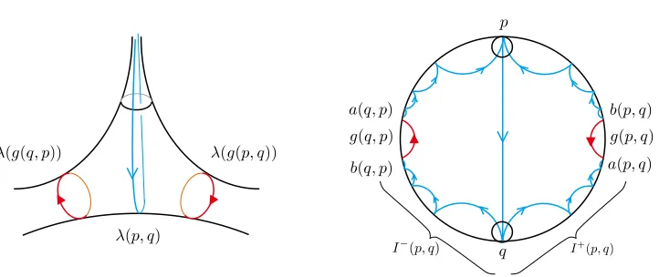
1. Then g(p, q)p=q and g(p, q)−1[p, q] is the closure of the lift ofλ(p, q) with endpointpwhich is closest to [p, q], among the lifts ofλ(p, q) with endpoint p, with respect to the preferred orientation of ˜τ. (See Figure 1.)
In the quotient surface Σ, the oriented closed geodesicλ(g(p, q)) is homotopic to the simple oriented loop obtained by shortcutting the oriented arc λ(p, q) by the horocyclic arc which is the image of the subarc of ˜τ bounded by s0 and s1. Thus
λ(g(p, q)) is a simple closed geodesic disjoint from the proper geodesic arcλ(p, q). In particular, [p, θ(p)q]∩ α(g(p, q)) = ∅. In fact, the map [(p, q) 7→ g(p, q)] : ∆−→ Γ is characterised by the following properties: for all (p, q) ∈ ∆, we have
g(p, q)p=q, g(q, p)g(p, q) =θ(p), and [p, θ(p)q]∩α(g(p, q)) =∅.
Write a(p, q) = a(g(p, q)) and b(p, q) = b(g(p, q)). Then the points p, a(q, p),
b(q, p), q, a(p, q),b(p, q) occur in this order around C. Let I+(p, q) = (q, a(p, q)),
I−(p, q) = (b(q, p), q) and I(p, q) = (b(q, p), a(p, q)) be open intervals in C. Thus
I(p, q) = I−(p, q)∪ {q} ∪I+(p, q), I(p, q)∩θ(p)nI(p, q) = ∅ for all n 6= 0, and I(p, q)∩θ(p)nI(q, p) = ∅ for all n.
In the quotient surface Σ, the oriented simple closed geodesics λ(g(p, q)) and
Figure 1. In the right figure, the two red arcs with thick arrows
represent the axesα(g(p, q)) and α(g(q, p)) of the hyperbolic trans-formationsg(p, q) and g(q, p) respectively. The blue arcs with thin arrows represent the oriented geodesic [p, q] and its images by the infinite cyclic groups hg(p, q)i and hg(q, p)i. The three intersection points of the blue arcs and the horocircle ˜τ centred at pare s−1, s0 and s1, from left to right.
the simple geodesic raysλ(p, a(p, q)) andλ(p, b(q, p)) emanating from the puncture spiral to λ(g(p, q)) and λ(g(q, p)), respectively. Thus, each of I±(p, q) projects homeomorphically onto a gap in the horocircle τ, in the sense of [Mcs, p.610]. In fact, each of I±(p, q) is a maximal connected subset of C\ {p} consisting of points x such that the geodesic ray λ(p, x) is non-simple. Moreover, if λ(p, x) is non-simple, thenx is contained in I±(p, q) for some q∈Π(p) (see [Mcs, TaWZ]). Write I(p) = {I(p, q) | q ∈ Π(p)}. Then we obtain the following as a conse-quence of [Mcs, Corollary 5] and [BiS] (see also [TaWZ, Section 5]):
Theorem 4.1. The elements of I(p) are pairwise disjoint. The complement, C\S
I(p), is a Cantor set of Hausdorff dimension 0.
Here, of course, the Hausdorff dimension is taken with respect to the euclidean metric on the horocycle, τ. Up to a scale factor, this is the same as the euclidean metric in the upper-half-space model with p at ∞. (Note that we could equally well use the circular metric on the boundary, C, induced by the Poincar´e model, since all the transition functions are M¨obius, and in particular, smooth.)
Write R(p) = {p} ∪ Π(p)∪ (C \S
I(p)) ⊆ C. This is a closed set, whose complementary components are precisely the intervalsI±(p, q) forq ∈Π(p). Thus the setR(p) is characterised by the following property: a pointx∈C\{p}belongs toR(p) if and only if the geodesic ray λ(p, x) in Σ is simple.
of parabolic points of Γ and {+,−}, respectively, by applying the loop cutting construction to the geodesic rayλ(p, x). To this end, we introduce a few notations. For p∈Π, we define maps (p), q(p) and g(p) from C\R(p) to {+,−}, Π(p) and Γ, respectively, by the following rule. If x ∈ C \R(p), then x ∈ I(p, q)
for some unique = ± and q ∈ Π(p). Define (p)(x) = , q(p)(x) = q, and g(p)(x) = g(p, q) or g(q, p)−1 according to whether = + or −. Note that the definition is symmetric under simultaneously reversing the orientation on C and swapping + with −.
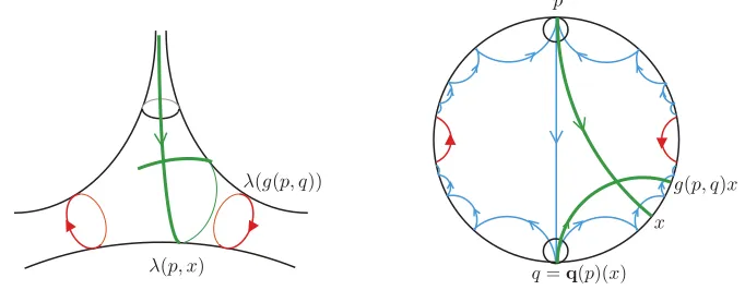
It should be noted that if x ∈ C \R(p), then, in the quotient surface Σ, the geodesic ray λ(q(p)(x), x) = λ(q, x) is obtained from the non-simple geodesic ray
λ(p, x) by cutting a loop, homotopic to λ(g(p)(x)) = λ(g(p, q)), and straight-ening the resulting piecewise geodesic (see Figure 2). (In the quotient, we are allowing ourselves to cut out any peripheral loops that occur at the beginning.) In particular, if x ∈ Π\R(p), then both λ(p, x) and λ(q(p)(x), x) are proper geodesic paths in Σ, and their self-intersection numbers satisfy the inequality
[image:9.612.134.475.334.467.2]ν(p, x)> ν(q(p)(x), x).
Figure 2. In the figure, we assume (p)(x) = + and so g(p)(x) = g(p, q).
We now fix, once and for all, somep∈Π. (Since the construction is equivariant with respect to the action of Γ, the choice does not ultimately matter. We will always get the same picture on projecting to Σ.)
By repeatedly applying the maps above, we associate for a given x ∈ C, a sequence (gi)i in Γ, (pi)i in Π, and (i)i in{+,−}as follows.
Step 0. Set p0 =p. (Thus, p0 is independent of x∈C.)
Step 1. If x∈R(p0), we stop with the 1-element sequence p0, and define (gi)i
and (i)i to be the empty sequence. If x /∈ R(p0), set g1 = g(p0)(x), p1 = g1p0,
1 =(p0)(x), and continue to the next step. (The sequences (gi)i and (i)i begin
with index i= 1.)
Step 2. If x ∈ R(p1), we stop with the 1-element sequences g1 and 1 and 2-element sequence p0, p1. If x /∈ R(p1), set g2 = g(p1)(x), p2 = g2p1 and 2 =
We continue this process, forever or until we stop.
We call the resulting sequences (gi)i, (pi)i and (i)i the derived sequences for x. More specifically, we call (gi)i and (pi)i thederived Γ-sequence and thederived
Π-sequence for x, respectively.
Lemma 4.2. Let x∈C, and let (gi)i, (pi)i and (i)i be the derived sequences for x. Then the following hold.
(1) The sequences (pi)i and (i)i are determined by the sequence (gi)i by the
following rule: pi = hip0 where hi = gigi−1· · ·g1, and i = + or − according to
whether gi =g(pi−1, pi) or g(pi−1, pi)−1.
(2) A point y ∈ C has the derived Γ-sequence beginning with g1, g2, . . . , gn for
some n≥1, if and only if y∈Tn
i=1I
(p
i−1, pi).
(3) Set R=S
p∈ΠR(p). If x /∈R, then the derived Γ-sequence (gi)i is infinite. (4) If x∈Π, then the derived Γ-sequence (gi)i is finite.
Proof. (1), (2) and (3) follow directly from the definition of the derived sequences. To prove (4), letx be a point in Π. Ifx∈R(p), then (gi)i is the empty sequence.
So we may assumex∈Π\R(p). Then by repeatedly using the observation made prior to the construction of the derived sequences, we see that the self-intersection number ν(pi, x) of the proper geodesic path λ(pi, x) is strictly decreasing. Hence ν(pn, x) = 0 for somen. This means thatx∈R(pn) and so the derived sequences
terminate atn.
The following is an immediate consequence of Lemma 4.2(2).
Corollary 4.3. Suppose thatx∈Chas derivedΓ-sequence beginning withg1, . . . , gn
for some n ≥ 1. Then there is an open set, U ⊆ C, containing x, such that if y∈U, then g1, . . . , gn is also an initial segment of the derived Γ-sequence for y.
Recall from Section 3 thatA(Γ,P, p) denotes the subgroup of Aut(Γ) preserving Π setwise and fixingp∈Π.
Lemma 4.4. Letφbe an element of A=A(Γ,P, p)withp=p0. Then the
follow-ing holds for every point x∈ C. If (gi)i, (pi)i and (i)i are the derived sequences
for x, then the derived sequences for φx are (φ(gi))i, (φpi)i and (deg(φ)i)i.
Here deg(φ) is the degree of the mapping class of Σ corresponding to φ: thus deg(φ) is +1 or−1 according to whetherφis induced by an orientation-preserving homeomorphism or by an orientation-reversing homeomorphism.
Proof. This can be proved through induction, by using the fact that the following hold for each φ ∈A.
(1) φ(R(p)) =R(p).
(2) For anyq∈Π(p), we have:
(a) If φ is orientation-preserving, then φ(θ(p)) = θ(p), φ(I(p, q)) =
(b) If φ is orientation-reversing, then φ(θ(p)) = θ(p)−1, φ(I(p, q)) = I−(p, φ(q)), φ(g(p, q)) =g(φq, p)−1, and φ(g(q, p)) = g(p, φq)−1.
5. Filling arcs
Let p = p0 be our chosen parabolic point. Let x be a point in C and (pi)i
the (finite or infinite) derived Π-sequence for x. Write λi = λ(pi−1, pi) for the
projection of [pi−1, pi]∩D to Σ. This is a proper geodesic arc in Σ. We call the
sequence (λi)i the derived sequence of arcs for x. We say that x is filling if the
arcs (λi)i eventually fill Σ, namely, there is somensuch that Σ\Sni=1λi is a union
of open discs. Let F be the subset of C consisting of points which are filling. In this section, we prove the following proposition.
Proposition 5.1. The set F is open in C, and its complement has Hausdorff dimension strictly less than 1. In particular, F has full measure.
We begin with some preparation. Let γ be a simple closed geodesic in Σ, and let X(γ) be the path-metric completion of the component of Σ\ γ containing the cusp. Then we can identify X(γ) as (H(G) ∩D)/G, where G = G(γ) is a subgroup of Γ containing Z = stabΓ(p), and H(G) ⊆ D ∪C is the convex hull of the limit set ΛG ⊆ C. In other words, X(γ) is the “convex core” of the hyperbolic surface H2/G, where G=G(γ) ∼=π
1(X(γ)) and p∈ΛG. To be more precise, pick a base point ˜∗ on a small horocircle ˜τ centred at p, and identify Γ with π1(Σ,∗) by using the base point, where ∗ is the image of ˜∗ in Σ. Then
G=G(γ) =j∗(π1(X(γ),∗))< π1(Σ,∗) = Γ, where j is the inclusion map.
Letδ be the closure of a component of∂H(G)∩D. This is a bi-infinite geodesic inD∪C. Let J ⊆C be the component of C\δ not containingp. Thus, J is an open interval inC, which is a component of the discontinuity domain of G. Note in particular, thatJ ∩Gp=∅.
Lemma 5.2. Suppose x ∈ J \R(p), and let g = g(p)(x), = (p)(x) and q = q(p)(x). Then, if g ∈G=G(γ), we have J ⊆I(p, q). In particular, g(p)(y) =g
for every y∈J.
Proof. To simplify notation we can assume (via the orientation-reversing symme-try of the construction) that = +. Note that q ∈ Gp⊆ ΛG, so [p, q] ⊆ H(G). Alsoα(g(p, q))⊆H(G) andδ⊆∂H(G). It follows that [p, q],α(g(p, q)) andδ are pairwise disjoint. Thus, J lies in a component of Y := C\ {p, q, a(p, q), b(p, q)}. Since = +, the four points, p, q, a(p, q), b(p, q) are located in C in this cyclic order, and so I+(p, q) = (q, a(p, q)) is a component of Y. Since J and I+(p, q) share the pointx, we obtain the first assertion that J ⊆I(p, q) with= +. The second assertion follows from the first assertion and the definition ofg(p)(y).
Lemma 5.3. Suppose that x ∈ J and that the derived Γ-sequence (gi)i for x is
Proof. Suppose, for contradiction, that gi ∈ G for all i. It follows that hi = gigi−1· · ·g1 ∈G for alli, and sopi =hip∈Gp⊆ΛGfor all i. By Lemma 5.2, we
have g(p)(y) = g(p)(x) = g1 for all y ∈ J. (Here (pi)i is the derived Π-sequence
for x and p= p0.) Now, applying Lemma 5.2 with p1 in place of p, we get that g(p1)(y) = g(p1)(x) = g2. Continuing inductively we get that g(pi)(y) = gi+1 for all i. In other words, the derived Γ-sequence for y is identical to that for x, and so, in particular, it must be infinite. We now get a contradiction by applying
Lemma 4.2(4) to any point y∈Π∩J.
If we takeBto be a standard horoball neighbourhood of the cusp, thenB∩γ =∅
for all simple closed geodesics in Σ, and so we can identifyB with a neighbourhood of the cusp in any X(γ).
Lemma 5.4. There is some θ <1 such that for each simple closed geodesic, γ, the Hausdorff dimension of ΛG(γ) is at most θ.
Proof. This is an immediate consequence of [FalM, Theorem 3.11] (see also [Mat, Theorem 1]) which refines the result of [Tu1], on observing that the groups G(γ) are uniformly “geometrically tight”, as defined in that paper. Here, this amounts to saying that there is some fixed r ≥0 (independent of γ) such that the convex core, X(γ), is the union of B and the r-neighbourhood of the geodesic boundary of the convex core. From the earlier discussion, we see that r is bounded above by the diameter of Σ\B, and so in particular, is independent of γ.
Let L ⊆ C be the union of the limit sets ΛG as G = G(γ) ranges over all subgroups of Γ obtained from a simple closed geodesic γ in Σ. Applying Lemma 5.4, we see that L is a Γ-invariant subset of C of Hausdorff dimension strictly less than 1. This is because it is a countable union of the limit sets ΛG whose Hausdorff dimensions are uniformly bounded by a constant θ <1.
Recall the set R = S
p∈ΠR(p) defined in Lemma 4.2(3). Then R is also Γ-invariant and has Hausdorff dimension zero by Theorem 4.1.
Lemma 5.5. If x∈C\(R∪L), then x is filling. Namely, C\(R∪L)⊆F.
Proof. Suppose, for contradiction, that some x∈C\(R∪L) is not filling. Then there must be some simple closed geodesic, γ, in Σ, which is disjoint from every
λi, where (λi)i is the derived sequence of arcs for the point x. Consider the
hyperbolic surface X(γ) and its fundamental group G= G(γ) ⊆Γ, as described at the beginning of this section. By hypothesis, x /∈ ΛG, and so x lies in some component, J, of the discontinuity domain of G. By Lemma 5.3, there must be some i∈Nwith gi ∈/ G. Choose the minimal suchi. Thus, hi−1 ∈Gbut hi ∈/G,
where hi =gigi−1· · ·g1. We have pi−1 =hi−1p∈Π∩ΛG and pi =hip∈Π\ΛG.
(The latter assertion can be seen as follows. Ifpi ∈ΛGthenpi is a parabolic fixed
point of G. Since X(γ) has a single cusp, there is an element f ∈ G such that
implies gi ∈ f G =G, a contradiction.) Therefore [pi−1, pi] meets ∂H(G), giving
the contradiction that λi crosses γ in Σ.
Proof of Proposition 5.1. By Lemma 5.5, we have C\F ⊆ R∪L. Since R and
L both have Hausdorff dimension strictly less than 1, the same is true of C\F. Thus, we have only to show that F is open. Pick an element x ∈F. Then there is some n such that Σ\Sn
i=1λi is a union of open discs, where (λi)i is a derived
sequence of arcs for x. By Corollary 4.3, there is an open neighbourhood U of x
in C such that every y∈ U shares the same initial derived Γ-sequenceg1, . . . , gn
with x. Thus, every y ∈ U shares the same beginning derived sequence of arcs (λi)ni=1 with x. Hence every y∈U is filling, i.e.,U ⊆F.
6. Wandering
In this section, we complete the proof of Theorem 2.2. To this end, we need the following lemma which appears to be well known, though we were unable to find an explicit reference.
Lemma 6.1. Let λ1, . . . , λn be a set of proper oriented arcs in Σ which together
fill Σ. Suppose that ψ is a mapping class on Σ fixing the proper homotopy class of each λi. Then ψ is trivial.
Proof. Fix any complete finite-area hyperbolic structure on Σ, and use it to iden-tify ˜Σ with H2. Construct a graph, K, as follows. The vertex set, V(K), is the set of bi-infinite geodesics which are lifts of the arcs λi for all i. Two arcs µ, µ0 ∈ V(K) are deemed adjacent in K if either (1) they cross (that is, meet in
H2), or (2) they have a common ideal point in ∂H2, and there is no other arc
in V(K) which separates µ and µ0. One readily checks that K is locally finite. Moreover, the statement that the arcsλi fill Σ is equivalent to the statement that K is connected. Note that Γ = π1(Σ) acts on K with finite quotient. Note also that K can be defined formally in terms of ordered pairs of points in S1 ≡ ∂H2
(that is corresponding to the endpoints of the geodesics, and where crossing is interpreted as linking of pairs). The action of Γ on K is then induced by the dynamically defined action of Γ on S1.
Now suppose that ψ ∈ Map(Σ). Lifting some representative of ψ and ex-tending to the ideal circle gives us a homomorphism of S1, equivariant via the corresponding automorphism of Γ. Suppose that ψ preserves each arc λi, as in
the hypotheses. Then ψ induces an automorphism, f : K −→ K. Given some
µ∈V(K), by choosing a suitable lift of ψ, we can assume thatf(µ) = µ.
We claim that this implies that f is the identity on K. To see this, first let
V0 ⊆V(K) be the set of vertices adjacent to µ. This is permuted by f. Consider the order on V0 defined as follows. Let IR and IL, respectively, be the closed
intervals of S1 bounded by ∂µ which lies to the right and left of µ. Orient each ofIR andIL so that the initial/terminal points ofµ, respectively, are those of the
such thatxR(ν) and xL(ν) are the endpoints ofν. Now we define the order≤ on V0, by declaring that ν ≤ ν0 if either (i) xR(ν) ≤ xR(ν0) or (ii) xR(ν) = xR(ν0)
and xL(ν)≤xL(ν0). This order must be respected by f, because f preserves the
orders onIR andIL. SinceV0 is finite, we see thatf|V0 is the identity. The claim now follows by induction, given thatK is connected.
It now follows that the lift of ψ is the identity on the set of all endpoints of elements of V(K). Since this set is dense in S1, it follows that it is the identity onS1, and we deduce that ψ is the trivial mapping class as required.
Recall that Map(Σ) is identified withM =A/Z, whereA=A(Γ,P, p) andZ =
Z(Γ, p), respectively, are the stabilisers of p in Aut(Γ,P) and Γ. As described in Section 3,Aacts onC\ {p}, and Map(Σ) =M acts on the circleT = (C\ {p})/Z. The wandering domainWM(T) is equal toWA(C\{p})/Z, becauseWZ(C\{p}) = C\ {p} (see Proposition 2.1).
Note that the set F in Proposition 5.1 is actually an open set of C\ {p}. For this setF, we prove the following lemma.
Lemma 6.2. F ⊆WA(C\ {p}).
Proof. We want to show that any x ∈ F has a wandering neighbourhood. By assumption, some initial segment, λ1, . . . , λn, of the derived sequence of arcs for x fills Σ. By Corollary 4.3, there is an open neighbourhood, U, of x, such that for every y∈U, the initial segment of length n of the derived sequence of arcs is identical with λ1, . . . , λn. Suppose that U ∩φU 6=∅ for some non-trivial element φ of Map(Σ) = A/Z. Pick a point y ∈ U ∩ φU and set x = φ−1y ∈ U. By assumption, the derived sequences of arcs for bothxand y begin withλ1, . . . , λn.
On the other hand, Lemma 4.4 implies that the derived sequence of arcs for
y =φx is equal to the image of that for x byφ. Hence we see that φλi = λi for
all i = 1, . . . , n. It follows by Lemma 6.1 below, that φ is the trivial element of
Map(Σ), a contradiction.
Proof of Theorem 2.2. By Proposition 5.1, F is an open set of C \ {p} whose complement has Hausdorff dimension strictly less than 1. Since WA(C \ {p})
containsF by Lemma 6.2, its complement inC\{p}also has Hausdorff dimension strictly less than 1. Since WM(T) = WA(C\ {p})/Z, this implies that the
non-wandering set,T \WM(T), has Hausdorff dimension strictly less than 1.
Remark 6.3. As noted in the introduction, one could allow Σ to have more than one cusp. In this case, we get an action of the pure mapping class group of Σ, (i.e. that which preserves the cusps) on the horocycle about any cusp. The construction is similar. We take Aut(Γ,P) to preserve each conjugacy class of peripheral subgroup, and Aut(Γ,P, p) to be the subgroup fixing a parabolic point
In the loop-cutting construction in Section 4, we need to allow g(p, q), for some (p, q) ∈ ∆, to be parabolic, so that a(p, q) = b(p, q) is a parabolic point (not in Π := Γp). The arguments of Section 4 then go through with some reinterpretation. Some further modification would be needed to Sections 5 and 6, though we will not elaborate on that here.
7. Notation
We summarise notations used in this paper.
◦ Σ = H2/Γ: a complete hyperbolic surface of finite area with precisely one puncture with Γ =π1(Σ).
◦ D= ˜Σ: the universal cover of Σ, which is identified with H2.
◦ C: the ideal boundary ofDwhich is equipped with a preferred orientation.
◦ Π ⊆C: the set of parabolic points of Γ.
◦ θ(p): the generator of stabΓ(p) which acts on C\ {p} as a translation in the positive direction.
◦ [x, y]⊆D∪C: the oriented geodesic from x toy for x, y ∈C.
◦ λ(x, y)⊆Σ: the image of [x, y]∩D in Σ.
◦ ν(p, q): the self-intersection number of the proper geodesic path λ(p, q), for p, q ∈Π.
◦ ∆ = {(p, q)∈Π2 |ν(p, q) = 0}={(p, q)∈Π2 |λ(p, q) is a proper geodesic arc}.
◦ For (p, q)∈∆;
– g(p, q)∈Γ: the element defined in Section 4.
– a(p, q), b(p, q): the attracting and repelling fixed points of g(p, q) respectively.
– α(g(p, q)) = [b(p, q), a(p, q)]: the axis of g(p, q).
– λ(g(p, q)): the oriented closed geodesic in Σ corresponding tog(p, q), i.e., the image of α(g(p, q))∩D in Σ.
– I(p, q) = I+(p, q)∪ {q} ∪I−(p, q) ⊆ C: the open interval defined in Section 4.
◦ For p∈Π;
– Π(p) ={q ∈Π|(p, q)∈∆}. – I(p) ={I(p, q)|q ∈Π(p)}. – R(p) = {p} ∪Π(p)∪(C\SI
(p))⊆C.
– (p), q(p), g(p): the maps from C \ R(p) to {+,−}, Π(p) and Γ, respectively, defined in Section 4.
◦ R =S
p∈ΠR(p)⊆C
◦ F ⊆C: the set of filling points.
◦ For a simple closed geodesic γ in Σ:
– X(γ): the path-metric completion of the component of Σ\γ contain-ing the cusp.
◦ L ⊆ C: the union of the limit sets ΛG as G = G(γ) ranges over all subgroups of Γ obtained from a simple closed geodesic γ in Σ.
References
[AkMS] H. Akiyoshi, H. Miyachi, M. Sakuma,Variations of McShane’s identity for punctured surface groups : Proceedings of the Workshop “Spaces of Kleinian groups and hyper-bolic 3-manifolds”, London Math. Soc., Lecture Note Series 329(2006) 151–185. [BiS] J. Birman, C. M. Series,Geodesics with bounded intersection are sparse: Topology24
(1985) 217–225.
[Bo1] B. H. Bowditch,A variation of McShane’s identity for once-punctured torus bundles : Topology 36(1997) 325–334.
[Bo2] B. H. Bowditch, Relatively hyperbolic groups : Int. J. Algebr. Comput. 22 (2012) 1250016, 66pp.
[FalM] K. Falk, K. Matsuzaki,The critical exponent, the Hausdorff dimension of the limit set and the convex core entropy of a Kleinian group : Conform. Geom. Dyn. 19 (2015) 159–196.
[FatLP] A. Fathi, F. Laudenbach, V. Po´enaru, et al,Thurston’s work on surfaces : Translated from the 1979 French original by D. M. Kim and D. Margalit, Mathematical Notes,
48, Princeton University Press, Princeton, 2012. xvi+254.
[K] T. Kuusalo,Boundary mappings of geometric isomorphisms of Fuchsian groups : Ann. Acad. Sci. Fenn. Math. Ser. A I Math. 545(1973) 1–7.
[Mas1] H. Masur, Interval exchange transformations and measured foliations : Ann. Math.
115(1982) 169–200.
[Mas2] H. Masur, Measured foliations and handlebodies : Ergod. Theory Dyn. Sys. 6(1986) 99-116.
[Mat] K. Matsuzaki, The Hausdorff dimension of the limit sets of infinitely generated Kleinian groups : Math. Proc. Camb. Phil. Soc.128(2000) 123–139.
[MccP] J. McCarthy, A. Papadopoulos,Dynamics on Thurston’s sphere of projective measured foliations, : Comment Math. Helv.64(1989) 133–166.
[Mcs] G. McShane,Simple geodesics and a series constant over Teichm¨uller space : Invent. Math. 132(1998) 607–632.
[OS] K. Ohshika, M. Sakuma,Subgroups of mapping class groups related to Heegaard split-tings and bridge decompositions : Geom. Dedicata180(2016) 117–134.
[TaWZ] S. P. Tan, Y. L. Wong, Y. Zhang,Generalizations of McShane’s identity to hyperbolic cone surfaces : J. Differential Geom.72(2006) 73–112.
[Tu1] P. Tukia, The Hausdorff dimension of the limit set of a geometrically finite Kleinian group : Acta Math.152(1984) 127–140.
[Tu2] P. Tukia,Hausdorff dimension and quasisymmetric mappings: Math. Scand.65(1989) 152–160.
Mathematics Institute, University of Warwick, Coventry CV4 7AL, Great Britain
Department of Mathematics, Graduate School of Science, Hiroshima Univer-sity, Higashi-Hiroshima, 739-8526, Japan