warwick.ac.uk/lib-publications
Original citation:
Charmoy, Philippe H. A., Croydon, David A. and Hambly, Ben M.. (2017) Central limit theorems for the spectra of classes of random fractals. Transactions of the American Mathematical Society.
Permanent WRAP URL:
http://wrap.warwick.ac.uk/75867
Copyright and reuse:
The Warwick Research Archive Portal (WRAP) makes this work by researchers of the University of Warwick available open access under the following conditions. Copyright © and all moral rights to the version of the paper presented here belong to the individual author(s) and/or other copyright owners. To the extent reasonable and practicable the material made available in WRAP has been checked for eligibility before being made available.
Copies of full items can be used for personal research or study, educational, or not-for-profit purposes without prior permission or charge. Provided that the authors, title and full
bibliographic details are credited, a hyperlink and/or URL is given for the original metadata page and the content is not changed in any way.
Publisher’s statement:
First published in Transactions of the American Mathematical Society. published by the American Mathematical Society. © 2017 American Mathematical Society.
A note on versions:
The version presented here may differ from the published version or, version of record, if you wish to cite this item you are advised to consult the publisher’s version. Please see the ‘permanent WRAP URL’ above for details on accessing the published version and note that access may require a subscription.
OF CLASSES OF RANDOM FRACTALS
PHILIPPE H. A. CHARMOY, DAVID A. CROYDON AND BEN M. HAMBLY
Abstract. We discuss the spectral asymptotics of some open subsets of the real line with random fractal boundary and of a random fractal, the continuum random tree. In the case of open subsets with random fractal boundary we establish the existence of the second order term in the asymptotics almost surely and then determine when there will be a central limit theorem which captures the fluctuations around this limit. We will show examples from a class of random fractals generated from Dirichlet distributions as this is a relatively simple setting in which there are sets where there will and will not be a central limit theorem. The Brownian continuum random tree can also be viewed as a random fractal generated by a Dirichlet distribution. The first order term in the spectral asymptotics is known almost surely and here we show that there is a central limit theorem describing the fluctuations about this, though the positivity of the variance arising in the central limit theorem is left open. In both cases these fractals can be described through a general Crump-Mode-Jagers branching process and we exploit this connection to establish our central limit theorems for the higher order terms in the spectral asymptotics. Our main tool is a central limit theorem for such general branching processes which we prove under conditions which are weaker than those previously known.
MSC:28A80 (primary), 60J80, 35P20 (secondary).
1. Introduction
Let D be a non-empty bounded open subset of Rd for d≥ 1 and let ∆ be the Dirichlet
Laplacian on D. Then the spectrum Λ of −∆ is discrete and forms a positive increasing sequence
0< λ1 ≤λ2 ≤ · · · ,
where the eigenvalues are repeated according to their multiplicity. Interest in the geometric information about D encoded by Λ started a little over 100 years ago and was crystallised by Kac in his paper [29] entitled ‘Can one hear the shape of a drum?’ Or more precisely, does Λ determineDup to isometry? The answer to that question is no in general, as shown in [21, 43]; see also [9] for a concise presentation of a family of counterexamples.
However some geometric information about D can be recovered. Weyl’s theorem shows that the eigenvalue counting function N defined by
N(λ) = #{λi :λi ≤λ}
has asymptotic expansion
N(λ) =c1(d)vold(D)λd/2+o(λd/2),
asλ→ ∞, for some constantc1(d) depending only ond, where volddenotes thed-dimensional
Lebesgue measure. Aside from prompting Kac’s question this result has led to a large body of work on the behaviour of the eigenvalue counting function and we now give a very brief description of the results that have motivated the work we will present here.
As a first extension it is natural to ask about the second order term in this expansion. If ∂Dis smooth, then under some assumptions, that there are not too many periodic geodesics, the expansion has a second order term
N(λ) =c1(d)vold(D)λd/2−c2(d)vold−1(∂D)λ(d−1)/2+o(λ(d−1)/2),
Date: December 6, 2016.
as λ → ∞, for some other constant c2(d) depending only on d. The reader is referred to
[26, 34, 46, 47, 50] and references therein for more information. This means that, under some regularity conditions, we can recover the size of the domain and that of the boundary from the spectral asymptotics; in particular, using the isoperimetric inequality, we can determine whether or not Dis an open ball.
Interest in the second term of the expansion of N grew further when Berry studied the spectral asymptotics of domains with a fractal boundary in [6, 7]. He conjectured that the Hausdorff dimension of ∂D should drive the second order term. Brossard and Carmona in [8] studied the associated partition function, a smoothed version of the eigenvalue counting function, and showed that the Minkowski dimension,dM, was the relevant notion of
dimen-sion for the second order term in the short time expandimen-sion of this function. For the counting function itself a general result of Lapidus [35] shows that, if d−1 < dM ≤ d, the second
order term is of order O(λdM/2) provided the Minkowski content of the boundary is finite. In general it is difficult to determine the precise order of growth for the second order term for arbitrary boundaries, however for one-dimensional domains [38] it was shown that the Minkowski dimension captures the order of growth of the second term in the asymptotics and the Minkowski content, the constant, when they exist.
The problem of determining the spectral asymptotics has also been considered for sets which are themselves fractal. For some classes of fractal, such as the Sierpinski gasket, or more generally p.c.f. self-similar sets [32] or generalised Sierpinski carpets [4], a Laplacian can be defined and shown to have a discrete spectrum. The exponent for the leading order growth rate in the eigenvalue counting function is called the spectral dimension and differs from the Hausdorff or Minkowski dimension of the set. If the fractal has enough symmetry, such as for instance the Sierpinski gasket, then a Weyl type theorem is no longer true [19], [5] in that the rescaled limit of the eigenvalue counting function does not converge. However the Weyl limit does exist for ‘generic’ deterministic p.c.f. self-similar sets [33] and also for random Sierpinski gaskets [23] and it is natural to ask about the growth of the second order term in these settings.
Our aim is to consider some random fractals where we anticipate more generic behaviour of the counting function. We will consider both domains with fractal boundaries and fractal sets here. Firstly we will consider the case of open subsets with fractal boundaries in the one-dimensional case of a so called fractal string. Our second case will be an example where the set itself is a fractal, the continuum random tree. In both cases the first order terms in the spectral asymptotics due to the fractal structure are understood and we will focus on the behaviour of the second order terms.
A fractal string is a set obtained as the complement of a Cantor set in the unit interval, so can be thought of as a sequence of intervals of decreasing length [37]. The Dirichlet Laplacian is then the union of the Dirichlet Laplacians on each interval. Some discussion of the spectral asymptotics of random fractal strings can be found in [24] where it is shown that for Cantor sets constructed via random iterated function systems, the second order term due to the boundary exists almost surely. We will consider a suitable subset of these random fractal strings and determine when the order of the fluctuations about the boundary term is given by a central limit theorem (CLT).
This turns out to be a subtle question and the existence of a CLT is determined by the rate of convergence in an associated renewal theorem. We will give a precise statement after introducing all the terminology in Theorem 4.3. We will then show that when the fractal is generated using a Dirichlet distribution, the existence of a central limit theorem depends on the particular Dirichlet distribution considered.
An example of what we are able to show is the following. LetSγ,α, forγ ∈(0,1), α∈N, be
interval and distributed as Dirichlet(α, α) (that is a Beta(α, α) distribution in this simple case) and 0< γ <1. We writePfor the probability law for the random fractal string andE
for expectation with respect toP. We note that γ will be the Minkowski dimension of the random Cantor setP-almost surely, that is the dimension of the boundary of the string. We write Nγ,α(λ) for the associated eigenvalue counting function.
Theorem 1.1. (i) For all α ∈ N and γ ∈ (0,1) there is a strictly positive deterministic constant C(γ, α) such that asλ→ ∞
λ−γ/2
1 πλ
1/2−N
γ,α(λ)
→C(γ, α) P-almost surely.
(ii) If α ≤59, then there exists a strictly positive deterministic constant σ(α) such that as
λ→ ∞
λγ/4
λ−γ/2
1 πλ
1/2−N
γ,α(λ)
−C(γ, α)
→Z, in distribution
where Z is normally distributed with mean 0 and variance σ(α)2∈(0,∞).
(iii) There exists an α >˜ 80 and a γ ∈ (0,1)such that: if 59 < α < α˜, then there exists a not-identically-zero periodic functionpγ,α(x) such that
ENγ,α(λ) =
1 πλ
1/2−C(γ, α)λγ/2+p
γ,α(logλ)λγη(α)/2+o(λη(α)),
where η(α) = max{<(θ0)∈(−∞,1) :P(θ0) = 0},
P(θ) :=
α−1 Y
i=0
(α+θ+i)−(2α)! α!
and, for this range of α we have 1/2< η(α)<1. In particular
λγ/4
λ−γ/2
1 πλ
1/2−N
γ,α(λ)
−C(γ, α)
does not converge in distribution asλ→ ∞.
Remark 1.2. (1) The first result gives the almost sure behaviour of the second term in the counting function asymptotics and is true for random fractal strings constructed using a wide class of distributions on the simplex.
(2) In part (iii) we conjecture that it is possible to take ˜α =∞ and any γ ∈(0,1). Indeed, towards proving the above result, we first provide conditions under which a CLT holds (see Theorem 4.3 and Section 5.2), and explain when one will not (see Remark 4.4). This distinction is determined by the rate of convergence in a related renewal theorem and depends on the values of the roots of P(θ) = 0, which we solve numerically (we can also solve this equation analytically for small values of α). These computations demonstrate that we can take ˜α to be at least 81. Furthermore, although we are not able to prove it rigorously, the monotonicity of the results suggests that ˜α can be taken arbitrarily large.
(3) We also conjecture that, in the case where there is no CLT, i.e. α >59, the size of the second order term is determined byη(α), in that,P almost surely for >0,
Nγ,α(λ) =
1 πλ
1/2−C(γ, α)λγ/2+O(λγη(α)/2+),
where 1/2< η(α)<1 and η(α)→1 as α→ ∞.
(4) The proof of the above result shows that the period ofpγ,αis given by 4π/γ|I(θ0)|, where
θ0 is one of the complex conjugate pair of roots whose real part givesη(α).
in the second order term in the counting function asymptotics [37]. Thus our result suggests that there is a non-trivial transition in the parameter space from the case where there is ‘enough randomness’ for a CLT about the second order term, to the case where there is not, through to the limit, where there is not even a strong law of large numbers for this term.
We will also consider the case of the Brownian continuum random tree, a random self-similar fractal. It was shown in [11] that there was a Weyl limit for the counting function in this case. It was also shown that the second order term for this fractal set was of order 1 in mean – which would be anticipated as the boundary of the tree is just two points, a 0-dimensional set. In this paper we show that there is a CLT about the almost sure asymptotics. However at this point we have not shown strict positivity of the variance due to the complexity of the correlation structure in the variance of the limit of the rescaled counting function. We conjecture that there will be a non-trivial CLT for this counting function. This will show that the randomness in the construction means the second order term in the spectral asymptotics is determined by the fluctuations about the leading order term, as these are much greater than the effects due to the boundary of the set.
The main technical tool we develop is a central limit theorem for the general Crump-Mode-Jagers branching process. In our setting the random fractal sets, the random Cantor set boundary of the string, or the continuum random tree, can be encoded as general branching processes. We are able to use a characteristic associated with these processes to determine the behaviour of the counting function. In this case there may be dependence on the offspring of an individual and we obtain a CLT in this more general setting, extending the work of [28]. We also remark that the techniques used here can easily be applied to geometric counting functions or other functions associated with heat flow, such as the partition function or heat content of the set. We anticipate similar behaviour in the fluctuations of these quantities about their almost sure limits.
The paper is organised as follows. In Section 2, we recall the definition of the general branching process and some laws of large numbers for such processes. We then prove our central limit theorem for the general branching process using a Taylor expansion proof. In Section 3, we restrict ourselves to general branching processes where a suitable function of the birth times is chosen to lie on an n-dimensional simplex, which will ensure that the limit of the usual branching process martingale is a constant. We will call such processes ∆n-GBPs and discuss extensively how to establish the conditions required for the central
limit theorem in this setting as this will allow us to illustrate when we do and do not have a central limit theorem for the associated general branching process. In Section 4, we define a family of open subsetsU of [0,1] whose random boundary is a statistically self-similar Cantor set built using scale factors on the simplex. We are then able to show our main result which gives conditions for the existence of a central limit theorem. In Section 5 we consider some examples where the law of the ∆n-GBP is given by a Dirichlet distribution. We show that,
for some Dirichlet weights, the eigenvalue counting function of the setU satisfies a central limit theorem. As a consequence we will be able to establish Theorem 1.1. In Section 6 we turn to the continuum random tree. We recall that this tree can be viewed as a random self-similar set and how to construct a Laplace operator on it. We then show that the conditions for the general branching process central limit theorem hold and hence there is a CLT in the spectral asymptotics.
Notation. For convenience, we will use the shorthand notationci withi∈Nto mean some
positive constant whose value is fixed for the length of a proof or a subsection.
2. A central limit theorem for general branching processes
In the general branching process, the typical individualxis born at timeσx, has offspring
whosebirth times are determined by a point process ξx on (0,∞), a lifetime modelled as a
non-negative random variableLx, and a (possibly random) c`adl`ag functionφx onRcalled a
characteristic.
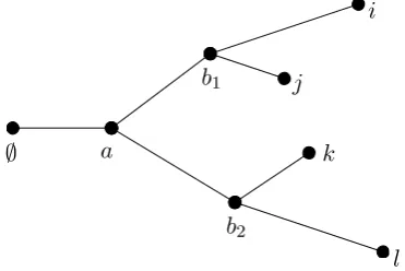
We index the individuals of the general branching process using the address space
(1) I = [
k≥0
Nk, where N0 =∅.
The ancestor ∅ is born at timeσ∅ = 0, and individual x hasξx(0,∞) offspring whose birth
times σx,i satisfy
ξx= ξx(∞)
X
i=1
δσx,i−σx,
where δ is the Dirac measure and x, i is the concatenation of x and i. The trace of the underlying Galton-Watson process is a random subtree ofI which we denote by Σ. We write ∂Σ for the set of infinite lines of descent in the process. Forx, y∈Σ we also use the notation x ≤y if there exists a sequence (z1, . . . , zk) with zi ∈N, i = 1, . . . , k with k∈ N such that
y = (x, z1, . . . , zk). Similarly, for x ∈ Σ, y ∈∂Σ we write x ≤ y if there exists a sequence
(z1, z2, . . .) with zi ∈ N, i = 1,2, . . . such that y = (x, z1, z2, . . .). A cut-set C of Σ is a
collection of x∈ Σ such thatx 6≤x0 and x0 6≤x for all x0 6=x ∈ C and ∀y∈ ∂Σ there is an x∈ C such that x≤y.
It is customary to assume that the triples (ξx, Lx, φx)xare i.i.d. but we allowφx to depend
on the progeny of x; we also do not make any assumptions on the joint distribution of (ξx, Lx, φx). When discussing a generic individual, it is convenient to drop the dependence
on x and write (ξ, L, φ). We will write P for the associated probability law and E for its expectation.
We define
ξ(t) =ξ((0, t]), ν(dt) =Eξ(dt), ξγ(dt) =e−γtξ(dt), and νγ(dt) =Eξγ(dt),
for γ ∈ (0,∞). Furthermore, we will always assume that the general branching process has Malthusian growth, i.e. that there exists a Malthusian parameter γ ∈ (0,∞) for which νγ(∞) = 1. This implies, in particular, that the general branching process is super-critical.
We denote the moments of the probability measureνγ by
(2) µk=
Z ∞
0
skνγ(ds).
In all cases of interest to us,µ1 will be finite. Note, however, that some convergence results
still hold when that is not the case, as explained in [45].
The presence of the characteristicφin the population is captured using thecharacteristic counting process Zφdefined as
(3) Zφ(t) =X
x∈Σ
φx(t−σx) =φ∅(t) + ξ∅(∞)
X
i=1
Ziφ(t−σi),
where theZiφ are i.i.d. copies ofZφ. An important example in the study of random fractals is the characteristicφ(t) = (ξ(∞)−ξ(t))1[0,∞)(t), whose corresponding counting processZφ
has the property that Zφ(t) is the number of offspring born after time t to parents born up to time t. Later, we will define characteristics that count eigenvalues of the Dirichlet Laplacian.
There are two central elements in the study of the asymptotics of the counting process. The first is that the functions
satisfy the well-studied renewal equation
(4) zφ(t) =uφ(t) +
Z ∞
0
zφ(t−s)νγ(ds);
see [18] for a classic exposition and [27, 30, 41] for alternative results. The second is the process defined by
Mt=
X
x∈Λt e−γσx,
where
Λt={x∈Σ : x= (y, i) for some y∈Σ, i∈N, andσy ≤t < σx}
is the set of individuals born after time tto parents born up to time t. The processM is a non-negative c`adl`ag Ft-martingale with unit expectation, where
Ft=σ(Fx, σx≤t) and Fx=σ({(ξy, Ly) :σy ≤σx});
we call it thefundamental martingale of the general branching process.
The martingale convergence theorem shows that Mt→M∞ ast→ ∞, almost-surely, for some random variableM∞. Furthermore, under anxlogx condition standard in the theory of branching processes,M is uniformly integrable. More precisely, in [13, 14], Doney proved the following result.
Theorem 2.1 (Doney). The following are equivalent:
(i) E[ξγ(∞)(logξγ(∞))+]<∞;
(ii) EM∞>0; (iii) EM∞= 1;
(iv) M∞>0 almost surely on the set where there is no extinction; (v) M is uniformly integrable.
Otherwise, M∞= 0 almost surely.
For technical reasons, it is often easier to apply renewal theory under the assumption that φvanishes for negative times. When that is not the case, we can set
(5) χx(t) =φx(t)1t≥0+
ξx(∞)
X
i=1
Zx,iφ (t−σi)10≤t<σi
so that
Zφ1[0,∞)(t) =χ∅(t) + ξ∅(∞)
X
i=1
Ziφ(t−σi)1t−σi≥0.
This means that Zφ1[0,∞) = Zχ, the counting process of the characteristic χ, and we can
then work with Zχ instead of Zφ because χ vanishes for negative times and Zχ and Zφ obviously have the same asymptotics ast→ ∞.
2.2. Application to statistically self-similar fractals. As discussed in [17, 22, 42], the general branching process provides a natural way to encode statistically self-similar sets. We outline this connection now.
To build a statistically self-similar set K, we start with the address space I defined in (1) and a non-empty compact set K∅. To each x ∈ I, we associate a random collection (Nx,Φx,1, . . .Φx,Nx)x∈I, whereNx is a natural number and Φx,i are contracting similitudes whose ratios we write Rx,i. We assume that the collection is i.i.d. in x.
The random numbers (Nx, x∈I) generate a random subtree Σ ofI defined by ∅ ∈Σ and
Forx=x1, . . . , xn∈Σ, define
Kx= Φx1 ◦ · · · ◦Φx1,...,xn(K∅) and K= ∞
\
n=1 [
|x|=n
Kx,
where |x|is the length of the word x. The set K has the intuitive property that it can be written as scaled i.i.d. copies of itself, namely,
K=
N
[
i=1
Φi(Ki),
whereK1, . . . , KN are i.i.d. copies ofK.
Let us emphasise that the choice of K∅ is not unique in general. However, for technical reasons discussed in [17], we make the following two assumptions. First, we assume that the sets (intKx, x∈Σ)form a net, i.e.
x≤y =⇒ intKy ⊂intKx
and also
intKx∩intKy =∅ if neitherx≤y nory ≤x;
the analogue of the open set condition for self-similar sets. Second, we assume that the construction of K is proper. i.e. that every cut-set C of Σ satisfies the condition: for every x∈ C, there exists a point inKx that does not lie in any other Ky with y∈ C.
The Hausdorff dimension of statistically self-similar sets is almost surely constant on the event that it is not empty and was calculated in [17, 22, 42]. It is given in the following result by a formula, the random analogue of that due to Moran [44] and Hutchinson [25] familiar from the deterministic setup.
Theorem 2.2. Let K be a statistically self-similar set. Write(N, R1, . . . , RN)for the
num-ber of similitudes and their ratios. Then, on the event that the set K is not empty,
dimK= inf
(
s:E N
X
i=1
Rsi
!
≤1
)
a.s.
To specify a general branching process corresponding to the random setK, we set
ξx = Nx
X
i=1
δ−logRx,i,
and Lx = supiσx,i−σx. With this parametrisation, the set Kx in the construction of K
corresponds to an individual born at timeσx and has sizee−σx. Furthermore, since
E
Z ∞
0
e−sxξ(dx) =E N
X
i=1
Rsi
!
,
the Malthusian parameterγ is equal to the Hausdorff dimension ofK by definition.
2.3. Laws of large numbers. Before we can prove our central limit theorem for the general branching process, we state Nerman’s laws of large numbers, proved in [45]. They are proved for non-negative characteristics with progeny dependence. In applications, if this is not the case, it suffices to write the characteristic as the difference of its positive and negative parts. We start with the weak law of large numbers. Recall that a measure is said to be lattice if its support is contained in a discrete subgroup ofR and non-lattice otherwise.
Theorem 2.3. Let (ξx, Lx, φx)x be a general branching process with Malthusian parameter
γ, where φ≥0 and φ(t) = 0 for t <0. Assume that uφ is directly Riemann integrable and thatνγ is non-lattice. Assume further that, for every t,
E
sup
u≤t
φ(u)
Then,
zφ(t)→zφ(∞) =µ−11
Z ∞
0
uφ(s)ds,
where µ1 is defined in (2), and
e−γtZφ(t)→zφ(∞)M∞, in probability,
as t→ ∞, whereM∞ is the almost sure limit of the fundamental martingale of the general
branching process. Furthermore, ifM is uniformly integrable, then the convergence also takes place in L1.
The strong law of large numbers requires the following additional regularity condition.
Condition 2.4. There exist non-increasing bounded positive integrable c`adl`ag functions g
and h on[0,∞) such that
E
sup
t≥0
ξγ(∞)−ξγ(t)
g(t)
<∞ and E
sup
t≥0
e−γtφ(t) h(t)
<∞.
This first part of the condition is satisfied if there exists a non-increasing bounded positive functiong such thatνγ(1/g) is finite, because then
ξγ(∞)−ξγ(t)
g(t) ≤
Z ∞
t
1
g(s)ξγ(ds)≤
Z ∞
0
1
g(s)ξγ(ds),
which has finite expectation. As such, this can be thought of as a moment condition that is weaker than imposing thatνγ have a finite second moment; takeg(t) =t−2∧1.
In particular, if the expected number of offspring is finite, this part of the condition is satisfied since, with the latter choice of g,
E
Z ∞
0
g(t)−1e−γtξ(dt)≤sup
t≥0
{(1∨t2)e−γt}Eξ(∞)<∞.
We can now state the strong law of large numbers.
Theorem 2.5. Let (ξx, Lx, φx)x be a general branching process with Malthusian parameter
γ, where φ≥0 and φ(t) = 0 for t <0. Assume that νγ is non-lattice. Assume further that
Condition 2.4 is satisfied. Then,
zφ(t)→zφ(∞) =µ−11
Z ∞
0
uφ(s)ds,
where µ1 is defined at (2), and
e−γtZφ(t)→zφ(∞)M∞, a.s.,
as t→ ∞, whereM∞ is the almost sure limit of the fundamental martingale of the general
branching process. Furthermore, ifM is uniformly integrable, then the convergence also takes place in L1.
Similar results have been proved by Gatzouras in the lattice case. We will not use them here and refer the reader to [20].
2.4. The central limit theorem. In [28], Jagers and Nerman proved a central limit the-orem for the general branching process under the assumptions that the characteristics are i.i.d. We now give a Taylor expansion proof of a similar result, but continue to allowφx to
depend on the progeny ofx. We start by introducing some additional notation.
Consider the general branching process (ξx, Lx,ζ¯x)x with Malthusian parameter γ. We
assume that ¯ζ is such that
¯
Z(t) :=Zζ¯(t)
We will use the rescaled version ˜Z of ¯Z defined by
(6) Z(t) =˜ e−γt/2Z(t) = ˜¯ ζ∅(t) + ξ(∞)
X
i=1
e−γσi/2Z˜
i(t−σi),
where ˜ζ(t) =e−γt/2ζ(t).¯
Finally, to have a proxy for the variance, we define
(7) V(t) = ¯Z(t)2 =ρ∅(t) + ξ(∞)
X
i=1
Vi(t−σi),
where
ρ∅(t) = ¯ζ∅(t)2+ 2 ¯ζ∅(t) ξ(∞)
X
i=1
¯
Zi(t−σi) + 2 ξ(∞)
X
i=1 X
j<i
¯
Zi(t−σi) ¯Zj(t−σj).
As V satisfies an equation of the form (3) which leads to the renewal equation (4), the functionsv and r defined by
(8) v(t) =e−γtEV(t) and r(t) =e−γtEρ(t) satisfy the renewal equation
(9) v(t) =r(t) +
Z ∞
0
v(t−s)νγ(ds).
Our central limit theorem requires two technical conditions which we discuss now.
Condition 2.6. There exists ∈(0,1/2)such that
e−γt/2 X
σx≤t ¯
ζx(t−σx)→0, in probability,
as t→ ∞.
This is a regularity condition on ¯ζ. In applications, we typically expect ¯ζ to satisfy a weak law of large numbers. Therefore, the sum should grow like eγt and we can expect that the condition is satisfied.
Condition 2.7. There exists κ∈(0,∞) such that
sup
t∈R
E{|Z˜(t)|2+κ}<∞.
This is a moment condition. In applications, it is convenient to check it for the third moment, i.e. when κ= 1, because that can be done using renewal arguments.
Theorem 2.8. Let (ξx, Lx,ζ¯x)x be a general branching process with Malthusian parameter
γ, where ζ¯is such that EZ(t) = 0¯ for everyt. Assume that v is bounded and that
v(t)→v(∞),
some finite constant, as t→ ∞. Assume further that Conditions 2.6 and 2.7 hold. Then,
˜
Z(t)→Z˜∞, in distribution,
as t→ ∞, where the distribution of Z˜∞ is characterised by EheiθZ˜∞i=Ehe−12θ2v(∞)M∞i.
In the proof, we will use that if z1, . . . , zn and w1, . . . , wn are complex numbers whose
modulus is bounded byC, then
(10)
n
Y
i=1
zi− n
Y
i=1
wi
≤Cn−1
n
X
i=1
|zi−wi|.
Proof. For ∈(0,1/2), iterating from (6), the definition of ˜Z, we get
(11) Z(t) =˜ X
σx≤t
e−γσx/2ζ˜
x(t−σx) +
X
x∈Λt
e−γσx/2Z˜
x(t−σx).
The first sum appearing in (11) can be rewritten as
e−γt/2 X
σx≤t ¯
ζx(t−σx)
which, by Condition 2.6, converges to 0 in probability ast→ ∞if we choose appropriately small. For the rest of the proof, we fix such a choice of .
We now consider the other sum appearing in (11), and show that it converges in distribu-tion to ˜Z∞ ast→ ∞. The result will then follow from Slutsky’s lemma. In other words, for θ∈R, we want to show that
(12) E
h
eiθ
P
x∈Λte
−γσx/2Z˜(t−σx)−e−12θ2v(∞)M∞i→0,
ast→ ∞. To do this, write, for anx0 ∈(0,1) that will be chosen below,
A,t=
sup
x∈Λt
|θe−γσx/2Z˜
x(t−σx)| ≤x0
,
and split (12) as
E
h
eiθ
P
x∈Λte
−γσx/2Z˜x(t−σx)− e−12θ
2v(∞)M
∞;Ac ,t
i
(13)
+E
h
eiθ
P
x∈Λte
−γσx/2Z˜x(t−σx)− e−12θ
2v(∞)P
x∈Λte
−γσx ;A,t
i
(14)
+Ehe−12θ
2v(∞)P
x∈Λte−γσx −e−21θ2v(∞)M∞;A ,t
i
. (15)
We will show that each of these terms converge to 0 ast→ ∞. Fixθ∈Rand δ ∈(0,1). Let x0 =x0(δ)∈(0,1) be such that
|ez−1−z| ≤δ|z| and
ez−1−z−z
2
2
≤δ|z|2,
whenever z∈Csatisfies |z| ≤x0. And let τ =τ(δ, θ)∈(0,∞) be such that fort≥τ,
x−0(2+κ)|θ|2+κsup
u∈R
E{|Z˜(u)|2+κ}e−γκt/2 ≤δ,
θ2kvk∞e−γt≤x0
and
|v(∞)−v(t/2)| ≤δ,
whereκ is given by Condition 2.7.
Let us start by dealing with (13). Fort≥τ,
P(Ac,t) =P
sup
x∈Λt
|θe−γσx/2Z˜
x(t−σx)|2+κ> x2+0 κ
≤P X
x∈Λt
|θ|2+κe−γσx(1+κ/2)|Z˜
x(t−σx)|2+κ ≥x2+0 κ !
which, by Markov’s inequality, is bounded by
(16)
x0−(2+κ)|θ|2+κe−γκt/2E "
X
x∈Λt
e−γσx|Z˜
x(t−σx)|2+κ
#
≤x−0(2+κ)|θ|2+κe−γκt/2E
" X
x∈Λt
e−γσxE{|Z˜
x(t−σx)|2+κ|Ft}
#
≤x−0(2+κ)|θ|2+κsup
u∈R
E{|Z(u)|˜ 2+κ}e−γκt/2
≤δ,
where we have used thatσx∈ Ft, that ˜Zx is independent ofFt and that EMt= 1. (This
is where we need to control the moment of order 2 +κfor some κ∈(0,∞).) Therefore, (13) is dominated by
2P(Ac,t)≤2δ. Since δ is arbitrary, it follows that
E
h
eiθ
P
x∈Λte−γσx/2Z˜x(t−σx)− e−12θ
2v(∞)M
∞;Ac ,t
i
→0,
ast→ ∞, as required.
To deal with (15), recall that
X
x∈Λt
e−γσx =M
t→M∞, a.s.,
ast→ ∞. Therefore, dominated convergence implies that
E
h
e−12θ2v(∞)
P
x∈Λte
−γσx
−e−12θ 2v(∞)M
∞;A ,t
i
→0,
ast→ ∞, as required.
We will spend the rest of the proof dealing with (14), which we rewrite as
E
" Y
x∈Λt
Eneiθe−γσx/2Z˜x(t−σx)1
Ax ,t Ft o − Y
x∈Λt
Ene−12θ
2v(∞)e−γσx
1Ax ,t Ft o #
using the conditional independence built into the branching structure, where
Ax,t={|θe−γσx/2Z˜
x(t−σx)| ≤x0}.
By (10), the term inside the expectation satisfies
(17) Y
x∈Λt
E
n
eiθe−γσx/2Z˜x(t−σx)1
Ax,t
Ft
o
− Y
x∈Λt
E
n
e−12θ
2v(∞)e−γσx
1Ax,t
Ft o ≤ X
x∈Λt
E
n
eiθe−γσx/2Z˜x(t−σx)1
Ax ,t Ft o
−Ene−12θ
2v(∞)e−γσx
1Ax ,t Ft o .
A Taylor expansion and the second order exponential estimate yield that
E
n
eiθe−γσx/2Z˜x(t−σx)1
Ax ,t Ft o
− E 1 +iθe−γσx/2Z˜
x(t−σx)−
1 2θ
2e−γσxZ˜
x(t−σx)2
1Ax ,t Ft
Furthermore,
E 1 +iθe−γσx/2Z˜
x(t−σx)−
1 2θ
2e−γσxZ˜
x(t−σx)2
1Ax ,t Ft
−Ene−12θ
2v(∞)e−γσx
1Ax ,t Ft o ≤ E n
iθe−γσx/2Z˜
x(t−σx)
1Ax ,t Ft o +
E 1−1
2θ
2e−γσxZ˜
x(t−σx)2−e− 1 2θ
2v(∞)e−γσx
1Ax ,t Ft . Now, since E h ˜
Zx(t−σx)
Ft
i
= 0,
reasoning as in (16) shows that
E
n
iθe−γσx/2Z˜
x(t−σx)
1Ax ,t Ft o = E n
iθe−γσx/2Z˜
x(t−σx)
1Ω\Ax ,t Ft o
≤x0E n
x−01|θ|e−γσx/2|Z˜
x(t−σx)|1Ω\Ax ,t
Ft
o
≤x0E n
x−0(2+κ)|θ|2+κe−γσx(1+κ/2)|Z˜
x(t−σx)|2+κ1Ω\Ax ,t
Ft
o
≤δe−γσx,
fort≥τ. And, since forx∈Λt we have
|v(∞)θ2e−γσx/2| ≤θ2kvk
∞e−γt≤x0,
a Taylor expansion and the first moment exponential estimate yield that
E 1−1
2θ
2e−γσxZ˜
x(t−σx)2−e− 1 2θ
2v(∞)e−γσx
1Ax ,t Ft ≤ E −1 2θ
2e−γσxZ˜
x(t−σx)2+
1 2θ
2v(∞)e−γσx
Ft +1 2δθ
2|v(∞)|e−γσx
≤θ2{|v(t−σx)−v(∞)|+δkvk∞}e−γσx.
Notice that, fort≥τ,
(18)
X
x∈Λt
θ2{|v(t−σx)−v(∞)|+δkvk∞}e−γσx
≤θ2 X
x∈Λt\Λt/2
δ(1 +kvk∞)e−γσx +θ2
X
x∈Λt∩Λt/2
(2 +δ)kvk∞e−γσx
≤δθ2(1 +kvk∞)Mt+θ2(2 +δ)kvk∞
X
x∈Λt∩Λt/2 e−γσx.
Together, (17) to (18) show that (14) is dominated by
(19) Eδ[1 +θ2(1 + 2kvk∞)]Mt
+E
θ2(2 +δ)kvk∞
X
x∈Λt∩Λt/2 e−γσx
.
Fixc∈(0,∞) large. For tlarge enough, by Lemma 3.5 of [45],
E
X
x∈Λt∩Λt/2 e−γσx
≤E
X
x∈Λt∩Λt+c e−γσx
→µ
−1
Z ∞
c
ast→ ∞. The limiting expression can be made arbitrarily small by choosingclarge enough. Therefore, the second term in (19) converges to 0. Since EMt = 1, the first term can also
be made arbitrarily small by adjustingδ. The result follows.
2.5. A word on the lattice case. The statement of Theorem 2.8 requires us to show that v(t) →v(∞). This is typically done using renewal theory. Recall that if νγ is lattice,
supported on bZ, say, then this convergence does not occur. Instead we typically get that,
for everyy,
v(y+bn)→g(y),
asn→ ∞, whereg(y) is ab-periodic function. In this case, the proof presented above shows that, for everyy,
˜
Z(y+bn)→Z˜∞(y), in distribution, asn→ ∞, where the distribution of ˜Z∞(y) is characterised by
E
h
eiθZ∞(y)i=Ehe−12θ2g(y)M∞i.
3. The central limit theorem for ∆n-general branching processes
In this section, we discuss applications of the central limit theorem to the general branching process under the assumption that the number of offspringξ(∞) is constant and equal ton, say, and that the birth times σ1, . . . , σn are distributed such that, for some fixed constant
γ ∈(0,∞), we have (e−γσ1, . . . , e−γσn) is a distribution on the simplex ∆
n inRn, i.e.
n
X
i=1
e−γσi = 1.
The latter assumption ensures that the fundamental martingaleM ≡1. We call a branching process with offspring distribution defined on the simplex in this way a ∆n-general branching
process. For simplicity, we also suppose throughout this section thatνγis non-lattice, though
as discussed in Section 2.5, we expect subsequential versions of the results below to hold if this is not the case. A basic example that we will return to is the case where the distribution of (e−γσ1, . . . , e−γσn) is Dirichlet(α
1, . . . , αn).
In this case our general branching process (ξx, Lx, φx)x, with Malthusian parameterγ, will
satisfy a weak law of large numbers, i.e.
e−γtZφ(t)→zφ(∞), in probability,
as t → ∞. We wish to describe the random fluctuations around the limit. To do this, we study the expression
(20) eγt/2
h
e−γtZφ(t)−zφ(∞)i=e−γt/2
h
Zφ(t)−eγtzφ(t)
i
+eγt/2[zφ(t)−zφ(∞)].
Our aim is to apply Theorem 2.8 to the first part of this expression. We will see that conditions making this possible ensure that the second term converges to 0. This will then produce a result on the fluctuations ofZφ(t) thanks to Slutsky’s lemma.
An outline of this section is that we begin by centring our characteristic in order to apply the central limit theorem of Section 2. We then show that in order to control the centred characteristic we need to control the rate of convergence in the associated renewal theorem.
3.1. Centring the process. To start, notice that, in the notation of Section 2,
is a centred characteristic counting process, if we define ¯ζ by
(21)
¯
ζ∅(t) =φ∅(t) + n
X
i=1
eγ(t−σi)zφ(t−σ
i)−eγtzφ(t)
=φ∅(t) + n
X
i=1
eγ(t−σi)[zφ(t−σ
i)−zφ(t)],
where we have used thate−γσ1+· · ·+e−γσn = 1. This representation can be used to get the following control on ¯ζ under an assumption on |zφ(t−σ
i)−zφ(t)|.
Lemma 3.1. Let (ξx, Lx, φx)x be a ∆n-general branching process. Assume that
|zφ(t)−zφ(∞)| ≤c1e−β1t∧c2,
for some positive constants c1, c2 and β1 ∈[0, γ]. Then,
|ζ(t)| ≤ |φ(t)|¯ + 2nc1e(γ−β1)t∧c2eγt
.
Proof. Notice that
|ζ¯∅(t)| ≤ |φ∅(t)|+ n
X
i=1
eγ(t−σi){|zφ(t−σ
i)−zφ(∞)|+|zφ(t)−zφ(∞)|}
≤ |φ∅(t)|+
n
X
i=1
c1e(γ−β1)(t−σi)∧c2eγ(t−σi)
+nc1e(γ−β1)t∧c2eγt
≤ |φ∅(t)|+ c1
n
X
i=1
e(γ−β1)(t−σi)∧c
2
n
X
i=1
eγ(t−σi)
!
+nc1e(γ−β1)t∧c2eγt
.
The result follows upon noticing that
n
X
i=1
e(γ−β1)(t−σi) =e(γ−β1)t n
X
i=1
e−(γ−β1)σi ≤ne(γ−β1)t,
and proceeding similarly for the other sum. This lemma and the decomposition in (20) show that understanding the rate of convergence ofzφ(t) to its limit in the renewal theorem is helpful for estimating the fluctuations ofZφ. 3.2. Convergence rate in the renewal theorem. Consider the renewal equation
(22) z(t) =u(t) +
Z ∞
0
z(t−s)F(ds),
where F is a non-lattice distribution function on [0,∞). The key to solving the renewal equation is the renewal measure
H= ∞
X
n=0
F∗n,
whereF∗n denotes the n-fold convolution ofF with itself, becausezis typically given by
z(t) =
Z ∞
0
u(t−y)H(dy);
see [18, 30] among others. The renewal theorem of [18] states that ifF has a finite mean µ1,
then
(23) H(t)∼µ−11t,
wheref(x)∼g(x) means that f(x)/g(x)→1 as x→ ∞. Under some regularity conditions on u, e.g. ifu is directly Riemann integrable, this can be used to show that
z(t)→z(∞) = 1 µ1
Z ∞
−∞
ast→ ∞; see [18].
The error in the linear approximation of the renewal function
(24) G(t) =H(t)−µ−11t
has been studied extensively. WhenF has a finite second momentµ2,
(25) G(t)→ µ2 2µ2
1
,
ast→ ∞.
The rate of convergence of G(t) to its limit in this case can be studied using the Fourier transformf of F defined by
f(w) =
Z ∞
−∞
ewsF(ds), w∈C.
We refer the reader to [18, 40, 48, 49] and references therein for proofs; see also Appendix B of [32] for a discussion of the lattice case. In particular, Stone proved the following theorem in [48].
Theorem 3.2(Stone). Suppose that there existsr1 ∈(0,∞) such thatf(w) is analytic and
6= 1 when <w∈(0, r1). Then, for everyr ∈(0, r1),
G(t)− µ2 2µ2
1
=O(e−rt),
as t→ ∞.
Since we aim to apply Lemma 3.1, we will be particularly interested in exponential rates of convergence ofz(t) to its limit. This rate of convergence is connected to that in Theorem 3.2 by the following lemma adapted from [12] which we include for convenience.
Lemma 3.3. Let z, u and F satisfy the renewal equation (22). Suppose that
z(t) =
Z ∞
0
u(t−y)H(dy)→µ−11
Z ∞
−∞
u(y)dy,
as t→ ∞. Then,
z(∞)−z(t) =µ−11
Z ∞
0
u(t+y)dy−
Z ∞
0
u(t−y)G(dy).
Proof. It suffices to notice that
z(∞)−z(t) =µ−11
Z ∞
0
u(t+y)dy+µ−11
Z ∞
0
u(t−y)dy−
Z ∞
0
u(t−y)H(dy),
and use the definition ofG.
3.3. Checking the conditions of the central limit theorem. Discussing the conditions of the central limit theorem involves finding growth estimates for ¯ζ which can be verified using Lemma 3.1. To be compatible with the framework of Nerman’s law of large numbers, we will focus on the situation where the characteristic vanishes for negative times; extensions will be discussed where needed. We start by looking at Condition 2.6.
Lemma 3.4. Let (ξx, Lx, φx)x be a ∆n-general branching process and let ζ¯be defined as in
(21). Assume that φ(t) = 0 for t <0 and that there exists a constant c1 >0 such that
|ζ(t)| ≤¯ c1eβ1t,
Proof. Let ∈(0, γ/2−β1). Then, for t≥0,
e−γt/2 X
σx≤t ¯
ζ(t−σi)
≤e(β1+−γ/2)te−t X σx≤t
c1.
By Theorem 2.3,
e−t X
σx≤t 1→ 1
µ1
Z ∞
0
e−γtdt= 1 γµ1
in probability,
ast→0. So the result follows since β1+ < γ/2.
Coupled with Lemma 3.1, this result hints that we should not expect to have a central limit theorem when zφ(t)−zφ(∞) does not decay at least as fast as e−γt/2, the threshold for the second term in the right-hand side of (20) to converge to 0. We will explain more precisely why this is sharp in Remark 4.4.
Let us now discuss the moment condition for the central limit theorem. The next lemmas discuss a set of sufficient assumptions for Condition 2.7 to be satisfied for the ∆n-GBP. We
introduce the function
ψ(θ) =E n
X
i=1
e−θγσi,
and note thatψ(1) = 1 and thatψ(θ) is strictly decreasing in θ.
Lemma 3.5. Let (ξx, Lx, φx)x be a ∆n-general branching process. Then, we have
E
" X
x∈Σ
e−yγσx
#
= ∞
X
k=0
ψ(y)k,
and the sum is finite ify∈(1,∞). Proof. By monotone convergence,
E
" X
x∈Σ
e−yγσx
#
= ∞
X
k=0
E
X
|x|=k
e−yγσx
.
Further, conditioning on the birth times, we get that
E
X
|x|=k
e−yγσx
=E
X
|x|=k−1
n
X
i=1
e−yγσxe−yγ(σx,i−σx)
=ψ(y)E
X
|x|=k−1
e−yγσx
.
Iterating this and summing over k proves the equality with the infinite sum. Noting that ψ(y)<1 for y∈(1,∞) completes the proof. Relying on this, we can produce the following estimate on the third moment of the scaled process ˜Z.
Lemma 3.6. Let (ξx, Lx, φx)x be a ∆n-general branching process. Assume thatφ(t) = 0 for
t <0, that
|ζ(t)| ≤¯ c1eγt/2 for t≥0
and that v is bounded. Then,
sup
t≥0
E|Z(t)|˜ 3 <∞.
Proof. Notice that
(26) Z¯(t)3 =W∅(t) + n
X
i=1
¯
where
W∅(t) = ¯ζ∅(t)3+ 3 ¯ζ∅(t)2 n
X
i=1
¯
Zi(t−σi) + 3 ¯ζ∅(t) n
X
i,j=1
¯
Zi(t−σi) ¯Zj(t−σj)
+
3 X
i,j,k=1 not all equal
¯
Zi(t−σi) ¯Zj(t−σj) ¯Zk(t−σk).
Therefore, it is clear that|Z¯(t)|3 is bounded by X
x∈Σ
|ζ¯x(t−σx)|3
(27)
+ 3X
x∈Σ
|ζ¯x(t−σx)|2 n
X
i=1
|Z¯x,i(t−σx,i)|
(28)
+ 3X
x∈Σ
|ζ¯x(t−σx)| n
X
i,j=1
|Z¯x,i(t−σx,i)| |Z¯x,j(t−σx,j)|
(29)
+X
x∈Σ
n
X
i,j,k=1 not all equal
|Z¯x,i(t−σi)| |Z¯x,j(t−σj)| |Z¯x,k(t−σk)|.
(30)
To prove the lemma, it is sufficient to check that e−3γt/2 times the expectation of each of these terms is bounded, which we do now.
To deal with (27), note that
e−3γt/2EX x∈Σ
|ζ¯x(t−σx)|3 ≤c31E X
x∈Σ
e−32γσx =c3
1
∞
X
k=0
ψ(3/2)k<∞,
thanks to Lemma 3.5.
Notice that our assumption on the boundedness ofv implies that
EZ¯(t)2 ≤c2eγt.
Therefore, we can control the term corresponding to (28) using that
e−3γt/2EX x∈Σ
|ζ¯x(t−σx)|2 n
X
i=1
|Z¯x,i(t−σx,i)|
≤c21e−3γt/2E
"
X
x∈Σ
eγ(t−σx)
n
X
i=1
E[ ¯Zx,i(t−σx,i)2|Fx]1/2
#
≤c21c2E "
X
x∈Σ
e−γσi
n
X
i=1
e−γσx,i/2
#
≤nc21c2
∞
X
k=1
ψ(3/2)k
<∞,
using thatσx,i ≥σx and Lemma 3.5.
To deal with (29), we proceed similarly to get that
e−3γt/2EX x∈Σ
|ζ¯x(t−σx)| n
X
i,j=1
≤ne−3γt/2EX x∈Σ
|ζ¯x(t−σx)| n
X
i=1
|Z¯x,i(t−σx,i)|2
≤n2c1c2
∞
X
k=0
ψ(3/2)k.
The similar argument needed to bound the term corresponding to (30) relies on the ob-servation that, ifi, j and k are not all equal, then, assuming without loss of generality that iis different, we have
E{|Z¯i(t−σi)| |Z¯j(t−σj)| |Z¯k(t−σk)||F∅}
=E{|Z¯i(t−σi)||F∅}E{|Z¯j(t−σj)| |Z¯k(t−σk)||F∅}
≤(E[ ¯Zi(t−σi)2|F∅])1/2(E[ ¯Zj(t−σj)2|F∅])1/2(E[ ¯Zk(t−σk)2|F∅])1/2.
Using this and reasoning as above then shows that
e−3γt/2EX x∈Σ
n
X
i,j,k=1 not all equal
|Z¯x,i(t−σx,i)| |Z¯x,j(t−σx,j)| |Z¯x,k(t−σx,k)|
≤n3c2
∞
X
k=0
ψ(3/2)k.
The proof is complete.
These results are easily combined to produce a version of the CLT for the case with weights on the simplex.
Theorem 3.7. Let (ξx, Lx, φx)x be a ∆n-general branching process such that φ(t) = 0 for
t <0. Assume that
|zφ(t)−zφ(∞)| ≤c1e−β1t,
for some β1 ∈(γ/2,∞), that
|φ(t)| ≤c2eβ2t,
for some β2 ∈ (0, γ/2), and that v is bounded with v(t) → v(∞) as t→ ∞. Then the CLT
holds in that
e−γt/2Zζ¯(t)→Z˜∞, in distribution,
as t→ ∞, where the distribution of Z˜∞ is normal with mean 0 and variance v(∞).
Proof. It follows from Lemmas 3.1, 3.4 and 3.6 that Conditions 2.6 and 2.7 are satisfied. This, with our other assumptions, gives the required conditions for Theorem 2.8.
4. Spectrum of random self-similar Cantor strings
In this section, we discuss the spectral asymptotics of a family of open subsets of [0,1] whose boundary is a random self-similar Cantor set generated using a distribution on the simplex, called ∆n-random Cantor strings. Spectral asymptotics for a variety of Cantor
strings have been studied extensively in [24, 38, 39, 36] and references therein. We specialise the discussion to ∆n-random Cantor strings here so that we can study the fluctuations of
Figure 1. First 4 iterations of the construction of K with the distribution
Dir(1,1,1) and γ = 0.6.
4.1. Construction. Choose γ ∈(0,1), n≥2 and consider the random vector (T1, . . . , Tn)
with a probability law on the simplex. Start with the unit intervalK0 = [0,1] and replace it
by nequally spaced intervals of length T11/γ, . . . , Tn1/γ. Replace each of these intervals by n
intervals created independently with the same procedure. Iterating indefinitely, we obtain a decreasing sequence of compact sets (Kj, j ≥0), andK =∩jKj is a statistically self-similar
Cantor set. Indeed, in the notation of Subsection 2.2, it suffices to set
(N, R1, . . . , RN) = (n, T11/γ, . . . , Tn1/γ);
the maps (Φ1, . . . ,ΦN) can easily be deduced from this. The corresponding general
branch-ing process (ξ, L) (no characteristic just yet) is obtained as described in Subsection 2.2. By construction this is a ∆n-general branching process and its Malthusian parameter isγ.
Fig-ure 1 depicts the first 4 iterations in the construction of the set K with the distribution Dir(1,1,1).
The set in which we are interested in this chapter isU = [0,1]\K, whose boundary isK by construction. Thanks to the Lindel¨of property, U is a countable union of intervals. As such,U is arandom string in the sense of [38, 39, 36] and references therein.
4.2. Fractal dimension. Consider the set U defined above and recall that the Hausdorff dimension of∂U =K isγ. Using Theorem 2.5, we now show that the Minkowski dimension of∂U exists and is also equal to γ almost surely.
Theorem 4.1. The Minkowski dimension of the ∆n-random Cantor string K is almost
surely equal to γ.
Proof. Consider the characteristic function defined by φ(t) =ξ(∞)−ξ(t).
The corresponding counting process Zφ counts the number of offspring born after time t to parents born up to time t. As such, Zφ(t) is an upper bound for the covering number N(e−t, K) of K with balls of radius e−t.
By the strong law of large numbers, we have
e−γtZφ(t)→ 1 µ1
Z ∞
0
Ee−γsφ(s)ds∈(0,∞), a.s.,
ast → ∞. This is easily used to check that dimMK ≤γ almost surely. The result follows since dimK =γ almost surely.
4.3. Spectrum of the Dirichlet Laplacian. Recall that the eigenvalue counting function for a domain D(or a countable union of domains) of Ris defined by
ND(λ) = #{eigenvalues of −∆≤λ}.
Following [41], we define ¯
ND(λ) =
1
πvol1(D)λ
1/2−N
The function ¯ND has the property that ifD1 and D2 are disjoint, then
(31) N¯D1∪D2(λ) = ¯ND1(λ) + ¯ND2(λ). Furthermore, forr ∈(0,∞), a change of variables shows that (32) N¯rD(λ) = ¯ND(r2λ).
In our applications of the central limit theorem, we will rely on the following assumption, which was discussed in the previous section.
Assumption 4.2. The rate of convergence in the renewal theorem satisfies
G(t)−µ
2+σ2
2σ2
≤c1e−β1t
for larget, for some β1 ∈(γ/2,∞)
We may now use the general branching process to study ¯NU.
Theorem 4.3. Let K be a ∆n-random Cantor string with dimension γ and consider the
stringU = [0,1]\K. Then,
λ−γ/2N¯U(λ)→N, a.s. and in L1,
as λ→ ∞, for some strictly positive constant N. Furthermore, if Assumption 4.2 holds, then
λγ/4(λ−γ/2N¯U(λ)−N)→Z in distribution,
asλ→ ∞, whereZ has a normal distributions with mean 0 and varianceσ2 for some strictly
positive constant σ.
Proof. Define the random variable S by
S = (1−R1− · · · −Rn)/(n−1).
By construction and the properties in (31) and (32), we have
¯
NU(λ) = (n−1) ¯NS[0,1](λ) +
n
X
i=1
¯
NRiUi(λ) = (n−1) ¯N[0,1](S
2λ) +
n
X
i=1
¯ NUi(R
2
iλ),
whereUi are i.i.d. copies ofU.
Now recall that the eigenvalues of −∆ for the unit interval [0,1] are (nπ)2. Therefore, ¯
N[0,1](λ) =π−1λ1/2− bπ−1λ1/2c,
which is bounded by 1∧(π−1λ1/2).
To use the general branching process, set
φ(t) = (n−1) ¯N[0,1](S2e2t) and Zφ(t) = ¯NU(e2t)
so that
Zφ(t) =φ∅(t) + n
X
i=1
Ziφ(t−σi),
where Ziφ are i.i.d. copies of Zφ and Zφ is the counting process of the characteristic φ. Furthermore, notice that
(33) 0≤φ(t)≤(n−1)et1t<0+c11t≥0 and Zφ(t)1t<0≤c2et1t<0,
for some positive constantsc1 and c2.
To establish the first statement of the theorem, we use (5) and set
χ(t) =φ(t)1t≥0+
n
X
i=1
Ziφ(t−σi)10≤t<σi,
Thanks to Theorem 2.5, this implies that
e−γtZχ(t)→µ−11
Z ∞
0
e−γsEχ(s)ds∈(0,∞), a.s. and inL1,
ast→ ∞. By definition, this means that
λ−γ/2N¯U(λ)→µ−11
Z ∞
0
e−γsEχ(s)ds, a.s. and inL1,
asλ→ ∞, as required.
Let us now prove the second part of the theorem under Assumption 4.2. Consider ¯ζφ and ¯
ζχ defined as in (21) using φand χ. Notice that ¯
Zχ :=Zζ¯χ(t) and Z¯φ:=Zζ¯φ(t)
are equal for t≥0. In particular, the corresponding variance functionsvχ(t) and vφ(t) are equal fort≥0. Furthermore, applying the fact that ( ¯ζxφ)x is i.i.d. together with the bounds
from Lemma 3.1, it follows that there are positive constants c, τ= (2β1−γ)∧γ such that
rφ(t) =e−γtE|ζ¯φ(t)|2 ≤ce−τ|t|. These observations and the renewal theorem of [41] imply that
(34) lim
t→∞v
χ(t) = lim t→∞v
φ(t) =µ−1 1
Z ∞
0
e−γtEζ¯φ(s)2ds=v(∞)∈(0,∞),
say.
Sinceχ is bounded and
(35) |zχ(t)−zχ(∞)| ≤c
2e−β1t
by Assumption 4.2 and Lemma 3.3, the conditions of Theorem 2.8 are satisfied. This implies that
eγt/2(e−γtZχ(t)−N)→N(0, v(∞)), in distribution,
ast→ ∞. Using the definition ofZχ, the decomposition in (20), (35) and Slutsky’s lemma completes the proof.
Remark 4.4. The arguments in the proof can be used to show that there cannot be a central limit theorem when the rate of convergence in the renewal theorem is not fast enough. Suppose that
zφ(t)−zφ(∞) =c1e−β1t+o(e−β1t),
as t → ∞, for some real constant c1. Then notice that the centring ¯ζφ introduced in (21)
and used in the proof of Theorem 4.3 satisfies
¯
ζ∅φ(t) =φ∅(t) + n
X
i=1
eγ(t−σi)[zφ(t−σ
i)−zφ(∞) +zφ(∞)−zφ(t)]
=φ∅(t) +c1e(γ−β1)t
n
X
i=1
e−(γ−β1)σi−e−γσi
!
+o(e(γ−β1)t)
=φ∅(t) +c1e(γ−β1)tR+o(e(γ−β1)t),
say, as t → ∞ (where the remainder is deterministic). Notice that R is a strictly positive random variable. In particular, for some 0 ∈ (0,∞), we have P(R ≥ 0) > 0. Therefore,
there existst0 such that, fort≥t0,
|ζ¯∅φ(t)|2≥ |ζ¯∅φ(t)|21R≥0 ≥ 1 2c
2
120e2(γ−β1)t1R≥0. This implies that, fort≥t0,
rφ(t) =e−γtE|ζ¯∅φ(t)|2 ≥ 1 2c
2 120e(γ
−2β1)tP(R ≥
If β1 ∈ (0, γ/2], then, by renewal theory, we cannot have a finite limiting variance in (34)
and in particular, no central limit theorem.
5. Dirichlet distributions
We now consider the case where the distribution on the simplex is the Dirichlet distribution and perform some explicit calculations to show the range of behaviour that is possible in our set up. In this set up the birth times are distributed as
(e−γσ1, . . . , e−γσn)∼Dir(α
1, . . . , αn),
where Dir denotes the Dirichlet distribution. We will describe this situation by saying that the ∆n-general branching process has Dirichlet weights α= (α1, . . . , αn) and write
α0 =α1+· · ·+αn,
as usual.
5.1. Explicit calculations with Dirichlet weights. In general, it is difficult to determine the solutions to f(w) = 1 needed to use Theorem 3.2. In some cases with Dirichlet weights which we discuss now, however, we can use the properties of the Gamma function to study f and deduce convergence rates for the renewal theorem.
LetX∼Dir(α) be a random vector inRn. It is well-known that, for every i,
Xi ∼Beta(αi, α0−αi),
where Beta denotes the Beta distribution. Recall that if Y ∼Beta(β1, β2) then
EYθ= B(θ+β1, β2) B(β1, β2)
,
where B is the Beta function, i.e.
B(x, y) = Γ(x)Γ(y) Γ(x+y). Therefore, we get that
(36) ψ(θ) =E
" n X
i=1
Xiθ
#
= Γ(α0) Γ(α0+θ)
n
X
i=1
Γ(αi+θ)
Γ(αi)
,
where the equation defines ψ. For the general branching process with Dirichlet weights defined above, it follows that
(37) f(w) =
Z ∞
−∞
ewsνγ(ds) =
Z ∞
−∞
e(w−γ)sν(ds) =E
" n X
i=1
e−γσi(1−w/γ)
#
=ψ(1−w/γ).
Ifα0−αi ∈Z for everyi, we can use that Γ(w+ 1) =wΓ(w) to reduce the functionψ to
a rational function which may be simpler to analyse. Notice that this assumption implies in particular that there exist somea∈Rand`i∈Zsuch that, for everyi, we haveαi =a+`i.
Therefore,
α0=a+`0 =α1+· · ·+αn=na+`1+· · ·+`n,
from which it follows that (n−1)a∈Z.
By definition ofGin (24) and writing F =νγ, we have
G∗F(t) =H∗F(t)−µ−11
Z ∞
0
(t−s)F(ds)
=H(t)−1t≥0−µ−11t+ 1
Denoting byg the Fourier transform of Gand f that ofF =νγ, we thus get that
g(w) = 1
1−f(w), w∈C.
Applying (36) and (37), for the general branching process with Dirichlet weightsαsatisfying α0−αi∈Zfor every i, the functionf can be written
f(w) =ψ(1−w/γ) =
n
X
i=1
1 Pi(w)
,
wherePi is a polynomial of degreeα0−αi. It follows that
g(w) =
Qn
i=1Pi(w)
Qn
i=1Pi(w)−Pni=1 Q
j6=iPj(w)
= 1 +
Pn
i=1 Q
j6=iPj(w)
Qn
i=1Pi(w)−Pni=1 Q
j6=iPj(w)
= 1 +R(w) Q(w),
say. It is easy to see that
degR <(n−1)α0 = degQ.
Now, decomposeg into partial fractions and write
g(w) = 1 +
q
X
i=1
Qi(w)
(w−ρi)mi
,
where (ρi, i≤q) are the roots ofQ with corresponding multiplicitiesmi and Qi are
polyno-mials with degQi < mi for everyi; in particular,
m1+· · ·+mq = (n−1)α0.
Recall that, fork∈Z+ and <(λ−r)<0,
Z ∞
−∞
eλttke−rt1t≥0dt=
Z ∞
0
tke(λ−r)tdt= k! (r−λ)k+1
and therefore that
(38)
Z ∞
0
eλt d
k
dtk
tke−rt
dt= k!λ
k
(r−λ)k+1.
Using this, it is easy to check that
G(dt) =δ0(t)dt+ X
<ρi≤0 ˜
Qi(t)eρit1t<0dt+ X
<ρi>0 ˜
Qi(t)e−ρit1t≥0dt,
where the ˜Qi are polynomials determined using (38) and satisfying deg ˜Qi< mi. Of course,
sinceF is supported on [0,∞), so is H and therefore, by definition ofG, we have
G(t)1t<0 =−µ−11t1t<0.
Putting this together shows that
(39) G(dt) =δ0(t)dt−µ−111t<0dt+ X
<ρi>0 ˜
Qi(t)e−ρit1t≥0dt,
Lemma 5.1. Assume that all the roots of Qare simple. Then,
G(t) =−µ−111t<0t+
µ2
2µ211t≥0+
X
<ρi>0 ci
ρi
e−ρit1
t≥0,
where ci = Res(g;ρi), the residue of g at ρi.
Since in this case none of the singularities can be removed and all have order one, all theci
are non zero. Furthermore, since ifρi is a root with residueci then ¯ρi is a root with residue
¯
ci as g( ¯w) = g(w), roots with the same real part cannot cancel out. In particular, in this
case, the result of Theorem 3.2 is sharp.
Proof. Since all the roots of Q are simple, we have
g(w) = 1 +
q
X
i=1
ci
w−ρi
,
where we must haveci= Res(g;ρi). Integrating (39) then shows that
G(t) =1t≥0−µ−111t<0t− X
<ρi>0 ci
ρi
1t≥0+ X
<ρi>0 ci
ρi
e−ρit1
t≥0.
Since F has a second moment, the result now follows from (25) after lettingt→ ∞.
5.2. Examples. Let us first discuss how the observations above enable us to establish the desired rate of convergence for some simple cases of Dirichlet weights.
Example 1.
Lemma 5.2. Consider the general branching processes with Dirichlet weights α described above. Assume that
α1 =· · ·=αn=
k
n−1, k∈ {1,2,3,4}, n≥2.
Then the Fourier transformf(w) of νγ is analytic and 6= 1 when <w∈(0, γ]. In particular,
G(t)− µ2
2µ21 =O(e −γt),
as t→ ∞.
Proof. Letting α=k/(n−1) a direct calculation gives
ψ(θ) =
k
Y
i=1
α+i
θ+α+i−1, θ >−α.
There is always a solution toψ(θ) = 1 atθ= 1 and all we require is that the other solutions are less than 0 to establish, via (37), thatf(w) is analytic and6= 1 on <w∈(0,(1 +α)γ).
Fork= 1, the only solution toψ(θ) = 1 isθ= 1.
Fork= 2, the other solution toψ(θ) = 1 is given byθ=−2(α+ 1). Fork= 3, the other solutions toψ(θ) = 1 are
θ=−3α+ 4 2 ±
1 2
p
−3α2−12α−8.
and k= 4 has solutions to ψ(θ) = 1 at
θ=−2α−4,−3 2−α±
1 2
p
−4α2−20α−15.
Figure 2. Phase plots of 1−f(γw) for α = 1, 2, 3, 10, 30 and 60. The
black line indicates the set {z ∈C:<z = 1/2}. The regions of the plot are {z∈C:<z and =z∈[−s, s]}fors= 5, 10, 10, 40, 50 and 50.
Analytic solutions for the solutions to the equationψ(θ) = 1 do not appear to be available for larger values of k.
Example 2.
Here we discuss the general branching process derived from the class of examples mentioned in the Introduction in which the Dirichlet weights are of the form α = (α, α) with α ∈ N.
We will establish the Theorem from the Introduction.
Thanks to Lemma 5.2, we know that ifα ≤4, as n= 2, then the Fourier transformf of νγ defined in (37) can be used to show that the rate of convergence in the renewal theorem
is sufficiently fast for the requirements of Theorem 2.8. In other words, the applicability of Theorem 2.8 depends on the regularity of the characteristic φ.
More generally we need to solve the equation
f(γ(1−θ)) =ψ(θ) = 2Γ(2α)Γ(α+θ) Γ(α)Γ(2α+θ) = 1. Asα∈Nthis is a polynomial equation and hence we seek roots of
α−1 Y
i=0
(θ+α+i) = 2(2α−1)! (α−1)! .
By letting w = 1−θ the rate of convergence in the renewal theorem is given by the root of 1−f(γw) with smallest strictly positive real part. We have computed these values numerically.
Figure 3. Phase plots of 1−f(γw) forα= 30,60,80. The black line indicates
the set {z ∈ C : <z = 1/2}. The region of the plot is {z ∈ C : <z ∈ [0,2] and=z∈[8,10]}.
roots of 1−f(γw) closest to the imaginary axis are ρ±'0.9951±9.1074i; when α= 60, they are
ρ±'0.4962±9.1027i; and whenα= 80, they are
ρ±'0.3718 + 9.0963i.
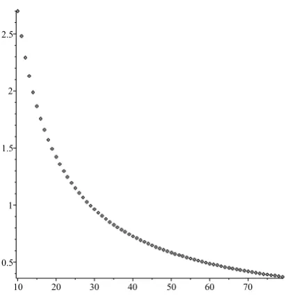
We have in fact computed the real part of the relevant root for all values of α from 1 to 80 – these are plotted in Figure 4. Numerically, this establishes that α = 60 is the smallest integer value for which 1−f(γw) has roots with real part<1/2.
Our computations also show that for 1≤α≤80 the roots of 1−f(γw) are all simple and occur as complex conjugate pairs except for the root at 0.
To summarise, this numerical evidence shows that the general branching process with Dirichlet weights (α, α) admits a central limit theorem of the type described when α ≤59, but not when 60≤α≤80. Moreover, the monotonicity of the plot in Figure 4 suggests that the range for which there is not a central limit theorem extends to allα≥60.
We note that we see similar results in the asymmetric case with Dirichlet weights (α1, α2),
α1, α2 ∈Nwith α2 ≤α1−1. In this case the polynomial equation becomes
α2−1 Y
i=0
(α1+θ+i)−
(α1+α2−1)!
(α1−1)!
!α1−α2−1 Y
i=0
(α2+θ+i) =
(α1+α2−1)!
(α2−1)!
.
Here is a table showing for a given α2 the values of α1 below which we are in the central
limit theorem regime.
α2 1 2 3 4 5 6 7 α1−1
α1 26 32 39 45 51 57 64 60
5.3. Applications to random self-similar strings. For the range of examples considered in Example 1 of Section 3, thanks to Lemma 5.2, we know that the Cantor set in Figure 1 satisfies Assumption 4.2 and so, by Theorem 4.3, the corresponding Cantor string satisfies a spectral central limit theorem.
We now return to the second example of Section 3, which was also discussed in the In-troduction. Figure 5 contains some pictures of statistically self-similar Cantor sets with Dirichlet weights (α, α) discussed in Subsection 5.2. The figure illustrates the fact that the geometry of the Cantor set becomes more rigid as α increases, because the corresponding Dirichlet distribution becomes more concentrated.

![Figure 3. Phase plots of 1[0the set−f(γw) for α = 30, 60, 80. The black line indicates {z ∈ C : ℜz = 1/2}.The region of the plot is {z ∈ C : ℜz ∈, 2] and ℑz ∈ [8, 10]}.](https://thumb-us.123doks.com/thumbv2/123dok_us/9434503.450427/27.595.96.502.75.199/figure-phase-plots-black-indicates-z-region-z.webp)