A second look at counting triangles in graph streams (corrected)

Original citation:

Cormode, Graham and Jowhari, Hossein. (2017) A second look at counting triangles in graph streams (corrected). Theoretical Computer Science, 683 . pp. 22-30.

Permanent WRAP URL:

http://wrap.warwick.ac.uk/97368

Copyright and reuse:

The Warwick Research Archive Portal (WRAP) makes this work by researchers of the University of Warwick available open access under the following conditions. Copyright © and all moral rights to the version of the paper presented here belong to the individual author(s) and/or other copyright owners. To the extent reasonable and practicable the material made available in WRAP has been checked for eligibility before being made available.

Copies of full items can be used for personal research or study, educational, or not-for-profit purposes without prior permission or charge. Provided that the authors, title and full bibliographic details are credited, a hyperlink and/or URL is given for the original metadata page and the content is not changed in any way.

Publisher’s statement:

© 2017, Elsevier. Licensed under the Creative Commons Attribution-NonCommercial-NoDerivatives 4.0 International http://creativecommons.org/licenses/by-nc-nd/4.0/

A note on versions:

The version presented here may differ from the published version or, version of record, if you wish to cite this item you are advised to consult the publisher’s version. Please see the ‘permanent WRAP url’ above for details on accessing the published version and note that access may require a subscription.

A Second Look at Counting Triangles in Graph Streams

(Revised)

Graham Cormode, Hossein Jowharia,b,

a_{[email protected], Corresponding author} b

[email protected]

Abstract

In this paper we present improved results on the problem of counting triangles in edge streamed graphs. For graphs with m edges and at least T triangles, we show that an extra look over the stream yields a two-pass streaming algorithm that usesO( m

ε2.5√_T polylog(m))space and outputs a(1 +ε)approximation of the

number of triangles in the graph. This improves upon the two-pass streaming tester of Braverman, Ostrovsky and Vilenchik, ICALP 2013, which distinguishes between triangle-free graphs and graphs with at least T triangle using O(_Tm1/3)

space. Also, in terms of dependence on T, we show that more passes would not lead to a better space bound. In other words, we prove there is no constant pass streaming algorithm that distinguishes between triangle-free graphs from graphs with at leastT triangles usingO(_T1/m2+ρ)space for any constantρ≥0.

1. Introduction

Many applications produce output in form of graphs, defined an edge at a time. These include social networks that produce edges corresponding to new friendships or other connections between entities in the network; communication networks, where each edge represents a communication (phone call, email, text message) between a pair of participants; and web graphs, where each edge repre-sents a link between pages. Over such graphs, we wish to answer questions about the induced graph, relating to the structure and properties.

networks, as they indicate common friendships: two friends of an individual are themselves friends. Counting the number of friendships within a graph is there-fore a measure of the closeness of friendship activities. Another use of the number of triangles is as a parameter for evaluation of large graph models [LBKT08].

For these reasons, and for the fundamental nature of the problem, there have been numerous studies of the problem of counting or enumerating triangles in var-ious models of data access: external memory [LWZW10, HTC13]; map-reduce [SV11, PT12, TKMF09]; and RAM model [SW05, Tso08]. Indeed, it seems that triangle counting and enumeration is becoming ade factobenchmark for testing “big data” systems and their ability to process complex queries. The reason is that the prob-lem captures an essentially hard probprob-lem within big data: accurately measuring the degree of correlation. In this paper, we study the problem of triangle counting over (massive) streams of edges. In this case, lower bounds from communication complexity can be applied to show that exactly counting the number of triangles essentially requires storing the full input, so instead we look for methods which can approximate the number of triangles. In this direction, there has been series of works that have attempted to capture the right space complexity for algorithms that approximate the number of triangles. However most of these works have fo-cused on one pass algorithms and thus, due to the hard nature of the problem, their space bounds have become complicated, suffering from dependencies on multiple graph parameters such as maximum degree, number of paths of length 2, number of cycles of length 4, etc.

In a recent work by Bravermanet al.[BOV13], it has been shown that at the expense of an extra pass over stream, a straightforward sampling strategy gives a sublinear bound that depends only onm(number of edges) andT (a lower bound on the number of triangles1_{). More precisely [BOV13] have shown that one}

ex-tra pass yields an algorithm that distinguishes between triangle-free graphs from graphs with at least T triangles using O(_Tm1/3) words of space. Although their

algorithm does not give an estimate of the number of triangles and more impor-tant is not clearly superior to theO(m_T∆)one pass algorithm by [PT12, PTTW13] (especially for graphs with small maximum degree∆), it creates some hope that perhaps with the expense of extra passes one could get improved and cleaner space

1_{In this and prior works, some assumption on the number of triangles is required. This is due}

in part to the fact that distinguishing triangle-free graphs from those with one or more triangle requires space proportional to the number of edges. Other works have required even stronger assumptions, such as a bound onT2, the number of paths of length 2, or the maximum degree of

complexities that beat the one pass bound for a wider range of graphs. In partic-ular one might ask is there a O(m_T) space multi-pass algorithm? In this paper, while we refute such a possibility, we show that a more modest bound is possible. Specifically here we show that the sampling strategy of [BOV13], namely uniform sampling of the edges at a rate of √1

T in the first pass and counting detected

trian-gles in the second pass gives aO(1)approximation of the number of triangles. To bring down the approximation precision to1 +ε, we use a simple summary struc-ture for identifying heavy edges (edges shared by many triangles which introduce large variance in the estimator) in order to deal with them separately from the rest of the graph. It turns out the right threshold forheavinessisO(pt/ε)which can be obtained from the two pass constant factor approximation. In order to avoid a third pass, we run the algorithm in parallel for different guesses of tand at the end pick the outcome of the guess that matches our constant factor approximation of t. We remark that a similar idea has been used in the recent work of Edenet al. [ELRS15] for approximately counting triangles in sublinear time. There, the notion of heaviness is applied to nodes, not edges, and the model allows query access to node degrees and edge presence. In our algorithm, we also utilize the one pass algorithm of Pagh and Tsourakakis [PT12] (explained below) as a sub-routine. Lastly, we observe that this m/√T dependence is attainable in one pass for a constant factor approximation—under the stronger assumption of random ordering of edge arrivals.

Furthermore, via a reduction to a hard communication complexity problem, we demonstrate that this bound is optimal in terms of its dependence on T. In other words there is no constant pass algorithm that distinguishes between triangle-free graphs from graphs with at leastT triangles usingO(_T1m/2+ρ)for any constant

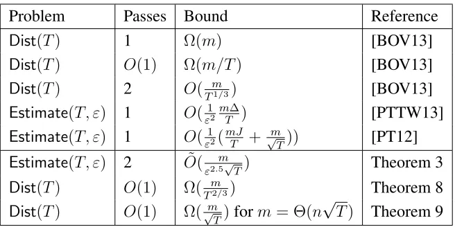
ρ > 0. Our results are summarized in Figure 2 and compared to other bounds in terms of the problem addressed, bound provided, and number of passes.

In line with prior work, we assume a simple graph—that is, each edge of the graph is presented exactly once in the stream. Note that our lower bounds immediately hold for the case when edges are repeated.

inci-dent on one node arrive together, or arrivals are randomly ordered, or adversarially ordered.

The work of Jowhari and Ghodsi [JG05] first studied the most popular of these combinations: insert-only, adversarial ordering. The general approach, common to many streaming algorithms, is to build a randomized estimator for the desired quantity, and then repeat this sufficiently many times to provide a guaranteed ac-curacy. Their approach begins by sampling an edge uniformly from the stream of m arriving edges onn vertices. Their estimator then counts the number of trian-gles incident on a sampled edge. Since the ordering is adversarial, the estimator has to keep track of all edges incident on the sampled edge, which in the worst case is bounded by ∆, the maximum degree. The sampling process is repeated O(_ε12

m∆

T )times (using the assumed lower bound on the number of triangles, T),

leading to a total space requirement proportial to O(_ε12

m∆2

T )to give an εrelative

error estimation of t, the (actual) number of triangles in the graph. The param-eter εensures that the error in the count is at most εt(with constant probability, since the algorithm is randomized). The process can be completed with a sin-gle pass over the input. Jowhari and Ghodsi also consider the case where edges may be deleted, in which case a randomized estimator using “sketch” techniques is introduced, improving over a previous sketch algorithm due to Bar-Yossef et al.[BYKS02].

The work of Buriolet al. [BFL+06] also adopted a sampling approach, and built a one-pass estimator with smaller working space. An algorithm is proposed which samples uniformly an edge from the stream, then picks a third node, and scans the remainder of the stream to see if the triangle on these three nodes is present. Recall thatnis the number of nodes in the graph,mis number of edges, and T ≤ tis lower bound on the (true) number of triangles. To obtain an accu-rate estimate of the number of triangles in the graph, this procedure is repeated independentlyO(_εmn2_T)times to achieverelative error.

Recent work by Pavan et al. [PTTW13] extends the sampling approach of Buriol et al.: instead of picking a random node to complete the triangle with a sampled edge, their estimator samples a second edge that is incident on the first sampled edge. This estimator is repeated O(m_ε2∆_T)times, where ∆represents the

maximum degree of any node. That is, this improves the bound of Buriol et al.

by a factor of n/∆. In the worst case,∆ = n, but in general we expect∆to be substantially smaller thann.

and then look for triangles induced by the sampled edges. Specifically, an al-gorithm which takes two passes over the input stream distinguishes triangle-free graphs from those withT triangles in spaceO(mT−1/3).

For graphs withW ≥mwhereW is the number of wedges (paths of length 2),

Jhaet al.[JSP13] have shown a single passO( m

ε2√_T)space algorithm that returns

an additive error estimation of the number of triangles where the estimation error is bounded byεW.

Pagh and Tsourakakis [PT12] propose an algorithm in the MapReduce model of computation, which depends on the maximum number of triangles on a single edge (J). However, it can naturally be adapted to the streaming setting. As de-scribed in Section 3, we make use of this algorithm as a subroutine in the design of our two pass algorithm. The space used by this algorithms scales asO(mJ_T +√m

T). Lower bounds for triangle counting. A lower bound in the streaming model is presented by Bar-Yossef et al. [BYKS02]. They argue that there are (dense) families of graphs over n nodes such that any algorithm that approximates the number of triangles must useΩ(n2_{)space. The construction essentially encodes} Ω(n2) bits of information, and uses the presence or absence of a single triangle to recover a single bit. Bravermanet al.[BOV13] show a lower bound ofΩ(m)

by demonstrating a family of graphs with m chosen between n and n2_{. Their}

construction encodes m bits in a graph, then adds τ edges such that there are eitherτ triangles or 0 triangles, which reveal the value of an encoded bit.

For algorithms which take a constant number of passes over the input stream, Jowhari and Ghodsi [JG05] show that still Ω(n/T) space is needed to approxi-mate the number of triangles up to a constant factor, based on a similar encoding and testing argument. Specifically, they create a graph that encodes two binary strings, so that the resulting graph hasT triangles if the strings are disjoint, and

2T if they have an intersection. In a similar way, Bravermanet al.[BOV13] en-code binary strings into a graph, so that it either has no triangles (disjoint strings) or at least T triangles (intersecting strings). This implies that Ω(m/T) space is required to distinguish the two cases. In both cases, the hardness follows from the communication complexity of determining the disjointness of binary strings.

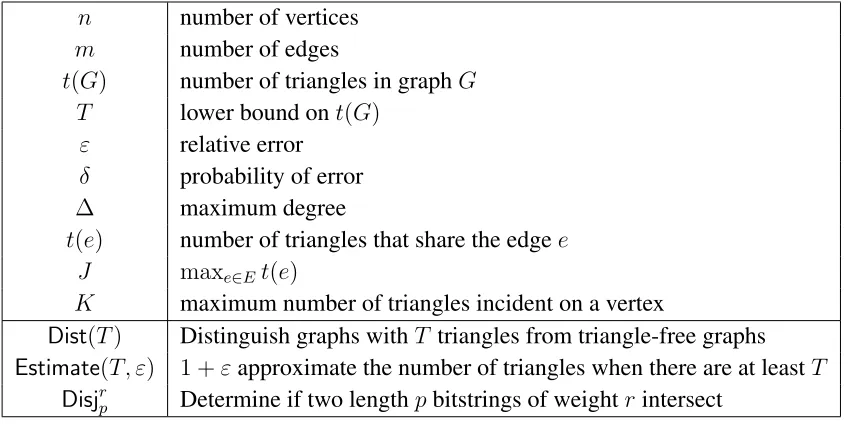
n number of vertices

m number of edges

t(G) number of triangles in graphG T lower bound ont(G)

ε relative error

δ probability of error

∆ maximum degree

t(e) number of triangles that share the edgee J maxe∈Et(e)

K maximum number of triangles incident on a vertex

Dist(T) Distinguish graphs withT triangles from triangle-free graphs

Estimate(T, ε) 1 +εapproximate the number of triangles when there are at leastT

Disjr_p Determine if two lengthpbitstrings of weightrintersect

Figure 1: Table of notation

algorithms. Our modified algorithm more directly handles heavy edges, and so can provide the claimed bounds.

2. Preliminaries and Results

In this section, we define additional notation and define the problems that we study.

As mentioned above, we uset(G)to denote the number of triangles in a graph G = (V, E). Let J(G) denote the maximum number of triangles that share an edge inG, andK(G)the maximum number incident on any vertex. We use t, J andKwhenGis clear from the context.

Problems Studied. We define some problems related to counting the number of triangles in a graph stream. These all depend on a parameter T that gives a promise on the number of triangles in the graph.

Dist(T): Given a stream of edges, distinguish graphs with at leastT triangles from triangle-free graphs.

Estimate(T, ): Given the edge stream of a graph with at least T triangles,

outputswhere(1−)·t(G)≤s≤(1 +)·t(G).

Problem Passes Bound Reference

Dist(T) 1 Ω(m) [BOV13]

Dist(T) O(1) Ω(m/T) [BOV13]

Dist(T) 2 O(_Tm1/3) [BOV13]

Estimate(T, ε) 1 O(_ε12

m∆

T ) [PTTW13]

Estimate(T, ε) 1 O(_ε12(

mJ T +

m

√

T)) [PT12]

Estimate(T, ε) 2 O˜(_ε2.m5√_T) Theorem 3

Dist(T) O(1) Ω(_Tm2/3) Theorem 8

Dist(T) O(1) Ω(√m

T)form = Θ(n

√

T) Theorem 9

Figure 2: Summary of results

T triangles. Consequently, we provide lower bounds for the Dist(T) problem, and upper bounds for the Estimate(T, )problem. Our lower bounds rely on the hardness of well-known problems from communication complexity. In particular, we make use of the hardness ofDisjr_p:

Problem 1 TheDisjr_pproblem involves two players, Alice and Bob, who each have

binary vectors of length p. Each vector has Hamming weightr, i.e. rentries set

to one. The players want to distinguish non-intersecting inputs from inputs that do intersect.

This problem is “hard” in the (randomized) communication complexity set-ting: it requires a large amount of communication between the players in order to provide a correct answer with sufficient probability [KN97]. Specifically,Disjr_p requires Ω(r) bits of communication for any r ≤ p/2, over multiple rounds of interaction between Alice and Bob.

Our Results. We summarize the results for this problem discussed in Section 1, and include our new results, in Figure 2. We observe that, in terms of dependence onT, we achieve tight bounds for 2 passes: Theorem 3 shows that we can obtain a dependence onT−1/2_{, and Theorem 9 shows that no improvement for constant}

passes as a function of T can be obtained. It is useful to contrast to the results of [PT12], where a one pass algorithm achieves a dependence of _Tm1/2, but has an

√

T triangles and handle them separately. Our results improve over the 2-pass bounds given in [BOV13]. Comparing with the additive estimator of [JSP13], while our sampling strategy is somewhat similar, using an extra pass over the stream we return a relative error estimation of the number of triangles.

Our analysis assumes familiarity with techniques from randomized algorithms: first, second and exponential moments methods, in the form of the Markov in-equality, Chebyshev inin-equality, and Chernoff bounds [MR95].

3. Upper bounds

In this section, we provide an upper bound in the form of a randomized al-gorithm which succeeds with constant probability. We begin by describing a 2-pass algorithm that outputs a constant factor approximation oft(G)using a lower boundT ont(G)(Section 3.1). Next we describe our main algorithm that uses the constant factor approximation algorithm as a sub-procedure and a summary of the graph (computed in the first pass) to improve the approximate factor to1 +ε (Sec-tion 3.3). We make use of the following result by Pagh and Tsourakakis [PT12].

Lemma 1 ([PT12]) Given a simple graph Gand arbitrary integer T, there is a

one-pass randomized streaming algorithm that outputs t0 such that|t0−t(G)| ≤

max{εT, εt(G)}. The expected space usage of the algorithm isO˜(_ε12(

mJ T +

m

√

T)),

whereJ denotes the maximum number of triangles incident on a single edge.

The algorithm of Lemma 1 works by conceptually assigning a “color” to each vertex randomly from C colors (this can be accomplished in the streaming set-ting with a suitable hash function, for example). The algorithm then stores each monochromatic edge, i.e. each edge from the input such that both vertices have the same color. Counting the number of triangles in this induced graph, and scal-ing up by a factor of C2 _{gives an estimator for t. The space used is O(m/C)}

in expectation. Setting C appropriately yields a one-pass algorithm with space

˜

O(_ε12(

m TJ +

m

√

T)).

3.1. Constant-factor approximation

The following simple lemma is a key observation in our algorithms. HereEh

is the set of all edgese∈Ewitht(e)≥h.

Lemma 2 The number of triangles that contain two or three edges from the set

Algorithm 1The(3 +ε)Algorithm

Repeat the followingl≥16/εtimes independently in parallel and output the min-imum of the outcomes.

Pass 1. Pick every edge with probability p =O( 1

ε4.5√_T)(with large enough

con-stants).

Pass 2. Definerto be the number of triangles that are observed where two edges

were sampled in the first pass, and the completing edge is seen in the second pass. Output _3p2₍₁r_−p).

PROOF: FromP_e∈Et(e) = 3tit follows that|Eh| ≤ 3_ht. Since every two distinct

edges belong to at most one triangle, the number of triangles that contain two or more edges fromEh is at most 3t/h₂

<(3_ht)2_.

Algorithm 1 describes our two-pass,(3 +ε)-factor approximation algorithm. Any use of this algorithm will set ε to be a constant, but for completeness our analysis makes explicit the dependence onε.

Theorem 3 Algorithm 1 is a 2-pass randomized streaming algorithm that uses

O( m

ε4.5√_T) space in expectation and outputs a (3 +ε) factor approximation of t

with constant probability.

PROOF: Let T represent the set of triangles in the graph. Consider one in-stance of the basic estimator, and let X be the outcome of this instance. Let Xi denote the indicator random variable associated with theith triangle inT

be-ing detected. By simple calculation, we have Pr[Xi = 1] = 3p2(1− p) and

E(X) = _3p2₍₁1_−p) P

i∈T Xi = t. Thus,X is an unbiased estimator fort; however,

R, which is the minimum of l independent repetitions of X, is biased. By the Markov inequality,Pr[X ≥(1 +ε)E(X)]≤1/(1 +ε). Therefore, pickingε≤1, we can conclude,

Pr[R ≤(1 +ε)t]≥(1−Pr[X ≥(1 +ε)t]16/ε)≥1− 1 2

16

≥1−10−4.

However, proving a lower bound onR is more complex, and requires a more involved analysis. First, we notice that most triangles share an edge with a limited

number of triangles. Let h =

q

9t

ε. We call Eh the set of heavy edges. LetTh

LetS =T/Th. For each trianglei∈S, fix two of its light (non-heavy) edges.

Let Yi denote the indicator random variable for the event where the algorithm

picks these two light edges of i ∈ S in the first pass. We haveE(Yi) = p2 and

always Yi ≤ Xi. Let Y = _p12 P

i∈SYi. Assumingp < 1, by definition we have

1/3Y < X. Therefore a lower bound onY will give us a lower bound onX. We have

E(Y) = |S| ≥(1−ε)t.

Also,

Var(Y) =E(Y2)−E2(Y)≤ 1

p2|S|+ 1

p|S| p

t/ε.

The first term comes from P

i∈S

1

p4E(Y

2

i ), and the second term arises from pairs

of triangles which share a light edge, of which there are at most |S|pt/ε(since the edge is light), and which are both sampled with probability p3_{. Using the}

Chebyshev inequality and assumingε < 1₂, we have

Pr[Y <(1−ε)2t] ≤ Pr[Y <(1−ε)|S|]

≤ Var(Y)

ε2_|S|2

≤ 1

ε2 1

p2_|S| +

p t/ε p|S|

!

< 1 ε2

2

p2_t + 2

p√εt

.

SinceT ≤ t, settingp > _ε3320.5√_T, allows the above probability to be bounded

by ₁₆₀ε . Now the probability that the minimum of16/εindependent trials is below the designated threshold is at most ₁₆₀ε 16_ε = 1/10. Therefore with probability at least 1−(1/10−4 _{+ 1/10) the output of the algorithm is within the interval} [1/3(1−2ε)t,(1 +ε)t]. This proves the statement of our theorem.

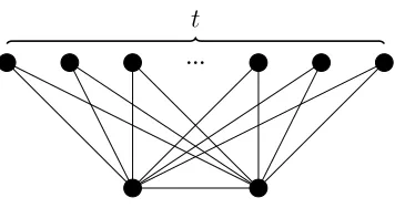
It can be shown the above analysis is tight2_{. Consider the “crown”-like graph}

wherettriangles share an edge shown in Figure 3. If we sample edges at a rate of p =O(√1

t), the bottom edge is picked with probabiltyp, an unlikely event. That

2_{An earlier version of this paper erroneously claimed that this algorithm achieved a 1 +ε}

t ...

Figure 3: “Crown”-like graph

Algorithm 2Constructing the summary structureSE(q, l)

Fori∈[l], in parallel.

• Sample each node independently with probabilityqintoSi.

• Ni ←all edges incident on any node inSi

means the random variable r will be concentrated around tp2 _{which divided by} 3p2_{(1−p)gives roughlyt/3as the estimate for number of triangles. On the other}

hand, fortdisjoint triangles,ris concentrated around3tp2(1−p)which divided by3p2_{(1−p)gives the right estimate for the number of triangles.}

3.2. Heavy-estimate data structure

Next we describe a simple summary structure of the graph which we refer to by SE(q, l)here. An instance ofSE(q, l)can be computed in one pass and can be used to decide whether an arbitrary edge of the graph is heavy or not in an approximate fashion. It is formed as a collection oflsets of edgesNi, chosen by

sampling as described in Algorithm 2. These sampled edges are used to estimate whether a given edgeemeets the heaviness condition, using Algorithm 3

We prove the following lemma regarding Algorithm 3.

Lemma 4 Letq ≥ 16

ε2_dandl =clognfor some constantc. The procedure

heavy-estimate(e) defined by Algorithm 3 can be used to decide whether t(e) ≥ d or

t(e)< 1₄dwith high probability. Moreover for every edge witht(e) ≥ d/4, t0(e)

approximatest(e)within a(1 +ε)factor.

PROOF: Fix an ordering on the triangles sharing e and let Xi,j be the random

Algorithm 3The heavy-estimate(e) procedure

Given edgee= (u, v)and summary structureSE(q, l)(sampled edge setsNi):

For eachi∈[l] :

ri(e)← |{w|(u, w)∈Ni ∧(v, w)∈Ni}|

(count the number of triangles formed betweeneandNi)

Returnt0(e) = medianiri(e)/qas estimate fort(e)

andXj is 1 ifw ∈Si We haveE[Xj] = qand thusE[ri(e) = P_jt(₌₁e) Xj] = qt(e).

Therefore,E[r(e)/q] =t(e). By a Chernoff bound,

Pr[|t0(e)−t(e))|> εt(e))]≤e−ε

2_qt(e)

4 .

Therefore, fort(e) ≥ d/4and choosingq ≥ 16

ε2_d, each estimatet

0_{(e)is close}

to the correct value with constant probability greater than 1/e. Hence, taking the median ofO(logn)instances gives us a value within the desired bounds with probability1−O(1/n2), via a standard Chernoff bound argument.

On the other hand, for edges witht(e) < 1

4d, the Markov inequality implies

that Pr[r(e)/q > d] < 1/4. The probability that the median ofΘ(logn) repeti-tions of the estimator goes beyonddisO(_n12).

3.3. Relative error approximation

To obtain a relative error guarantee, we overlap the execution of three algo-rithms in two passes, as detailed in Algorithm 4. Note that to optimize the de-pendence on ε, the parameters used to invoke each of the Algorithms 1 and 3 are carefully chosen.

Theorem 5 Algorithm 4 is a 2-pass randomized streaming algorithm that takes

O( m

ε2.5√_T polylog(n))space in expectation and outputs a(1 +ε)factor

approxi-mation oft(G).

PROOF:

In the following, for the sake of simplicity in exposition, we assume the ran-domized procedures used in the algorithm do not err. With appropriate choice of parameters the total error probability can always be bounded by a constant smaller than1/2.

As in Algorithm 4, letj = max{b ∈B|b≤t0}. LetEj be the set of edges

Algorithm 4Relative Error Algorithm Do the following tasks in parallel:

• Run Algorithm 1 withε= 1/12to findt0 such that1/4t≤t0 ≤t.

• Run Algorithm 3 to compute SE(q, l) for q = Θ(ε−1.5_T−0.5_{) and l =} Θ(logn).

• LetB ={T,2T,4T, ...,2i_{T}whereiis the smallest integer such that2}i_{T ≥}

n3_.

In the second pass, instantiate |B| parallel instances of the algorithm PTb

with parametersT = b, J = 24pb/εfor allb ∈ B. Also initiate counters

{hb}b∈B with zero.

Upon receiving the edgee∈E, first computet0(e)using the heavy-estimate procedure. For allb∈B, ift0(e)≥d= 24pb/ε, we addt0(e)to the global counterhb, otherwise we feedeto PTb.

At the end of the pass, lettb be the output of PTb. We outputhj +tj as the

final estimate for the number of triangles wherej = max{b ∈B|b≤t0}.

graphGafter removing the edgesEj. Lett(Ej)be the number of triangles inG

that share at least an edge withEj. Clearlyt(G) =t(Ej) +t(Gj).

First, we prove thathj is indeed a1 +O(ε)approximation oft(Ej). A source

of error comes from the fact that we will be over-counting triangles that have more than one heavy edges. We show that number of such triangles is limited. To see this, observe that with the choice of parameters q = Θ(ε−1.5T−0.5) and d = 3

q

t

2ε in Lemma 4, it follows that for eache∈ Ej we havet(e)≥6

q

j ε and

consequently t(e) ≥ 3q t

2ε. The latter follows from the fact that t/8 ≤ j ≤ t.

But, by Lemma 2, the number of triangles that have two or three heavy edges that

are shared by more than3

q

t

2ε is at mostεt. Another source of error comes from

estimation errors |t(e)−t0(e)|. This is also negligible since, by Lemma 4, for every identified heavy edgee, we have|t(e)−t0(e)|bounded byεt(e).

On the other hand, the maximum number of triangles on an edge for graphGj

is at mostO(

q

j

ε). Hence by Lemma 1,tj estimatest(Gj)withinεtadditive error

error. Rescalingεgives the desired result.

It remains to show that the expected space usage of the algorithm is bounded as claimed. The SE(q, l)summary takes O(nqm_n) = O(_ε1.m5√_T)in expectation.

The constant factor approximation takes O(m/√T) space. The instance of the

PT algorithm with parameter b takes O(m √

b/ε ε2_b +

m

ε2√_b) in expectation which is

bounded byO( m

ε2.5√_T)asT ≤b.

3.4. One pass algorithm

It is natural to ask whether this algorithm can be reduced to a single pass. There are several obstacles to doing so. Primarily, we need to determine for each edge whether or not it is heavy, and handle it accordingly. This is difficult if we have not yet seen the subsequent edges which make it heavy. We can adapt Algorithm 1 to one pass to obtain a constant factor approximation, under the as-sumption of a randomly ordered stream.

Corollary 6 Assuming the data arrives in random order, there is a one-pass

ran-domized streaming algorithm that returns a1/3 +εfactor approximation oft(G)

that usesO( m

ε4.5√_T)space.

PROOF: Under random order, we can combine the first and second passes of Algorithm 1. That is, we sample edges with probabilityp, and look for triangles observed based on the stream and the sample. We count all triangles formed as r: either those with all three edges sampled, or those with two edges sampled and the third observed subsequently in the stream. The estimator is now _pr2, since the

probability of counting any triangle isp3 _{(for all three edges sampled) plusp}2₍₁₋

p)(for the first two edges in the stream sampled, and the third unsampled). The same analysis as for Theorem 3 then follows: we partition the edges in to light and heavy sets, and bound the probability of sampling a subset of triangles. A triangle with two light edges is counted if both light edges are sampled, and the heavy edge arrives last. This happens with probabilityp2_{/3. We can nevertheless argue}

that we are unlikely to undercount such triangles, following the same Chebyshev analysis as above. This allows us to conclude that the estimator is good.

3.5. Non-simple graphs

All our algorithms can be modified to work when the graphs are not simple. That is, we may see the same edge multiple times in the graph stream, but are only interested in counting each unique triangle once. We need two tools to accomplish this: (1) hash functions which map nodes or edges to real numbers in the range

[0. . .1] and can be treated as random (2) count-distinct algorithms which can approximate the number of unique items (tuples of nodes) that are passed to them, up to a(1 +ε)factor.

The transformation of the algorithms is to replace sampling with hashing and testing if the hash value is less than the thresholdp. This has the effect of sampling each unique edge (or node) with probabilityp. We replace counting triangles with a count-distinct of the triangles.

For example, Algorithm 1 uses hashing to determine which (distinct) edges to sample in pass 1, then approximately counts the set of distinct triangles in pass 2. The one-pass algorithm of Lemma 1 can correspondingly be modified, as can Algorithm 3. The main change needed for Algorithm 4 is that we should extract the setof triangles counted in each invocation of Algorithm 3, and pass these to an instance of a count-distinct algorithmhb. Consequently, our results also apply

to the case of repeated edges. The space cost increases due to replacing counters with approximate counters. In each algorithm, the number of instances of count-distinct algorithms is small. Hence, these modifications increase the space cost by an additionalO˜(1/ε2), which does not change the asymptotic bounds.

4. Lower bounds

We now show lower bounds for the problemDist(T), to distinguish between the caset = 0andt ≥ T. Our first result builds upon a lower bound from prior work, and amplifies the hardness. We formally state the previous result:

Lemma 7 [BOV13] Every constant pass streaming algorithm for Dist(T)

re-quiresΩ(m_T)space.

Theorem 8 Any constant pass streaming algorithm forDist(T)requiresΩ(_Tm2/3)

space.

PROOF: Given a graph G = (V, E)with m edges we can create a graph G0 =

edge set{u1, . . . , uT} × {v1, . . . , vT}. Clearly any triangle inGwill be replaced

by T3 triangles in G0 and every triangle in G0 corresponds to a triangle in G. Moreover this reduction can be peformed in a streaming fashion usingO(1)space. Therefore a streaming algorithm forDist(T)usingo(_Tm2/3)(applied toG

0_{) would}

imply ano(m)streaming algorithm forDist(1). But from Lemma 7, we have that Dist(1)requiresΩ(m)space for constant pass algorithms. This is a contradiction and as a result our claim is proved.

Our next lower bound more directly shows the hardness by a reduction to the hard communication problem ofDisjr_p.

Theorem 9 For any ρ > 0 and T ≤ n2_{, there is no constant pass streaming}

algorithm forDist(T)that takesO(_T1m/2+ρ)space.

PROOF: We show that there are families of graphs with Θ(n

√

T) edges and T triangles such that distinguishing them from triangle-free graphs in a constant number of passes requiresΩ(n)space. This is enough to prove our theorem.

We use a reduction from the standard set intersection problem, here denoted byDisjn/_n 2. Giveny ∈ {0,1}n_{, Bob constructs a bipartite graphG= (A∪B, E)}

whereA = {a1, . . . , an}andB = {b1, . . . , b√_T}. He connectsai to all vertices

in B iff y[i] = 1. On the other hand, Alice adds vertices C = {c1, . . . , c√T}

to G. She adds the edge set C ×B. Also for each i ∈ [√T] and j ∈ [n], she adds the edge(ci, aj)iffx[j] = 1. We observe that ifxandy(uniquely) intersect

there will be precisely T triangles passing through each vertex of C. Since there is no edge between the vertices in C, in total we will have T triangles. On the other hand, if x andy represent disjoint sets, there will be no triangles inG. In both cases, the number of edges is between2n√T and3n√T, overO(n)vertices (using the boundT2 ≤n). Considering the lower bound for theDisjr_p(Section 2), our claim is proved following a standard argument: a space efficient streaming algorithm would imply an efficient communication protocol whose messages are the memory state of the algorithm.

Acknowledgments. We thank Andrew McGregor, Srikanta Tirthapura and Vladimir

[BFL+_{06] Luciana S. Buriol, Gereon Frahling, Stefano Leonardi, Alberto}

Marchetti-Spaccamela, and Christian Sohler, Counting triangles in

data streams, PODS, 2006, pp. 253–262.

[BOV13] Vladimir Braverman, Rafail Ostrovsky, and Dan Vilenchik, How

hard is counting triangles in the streaming model?, ICALP (1), 2013,

pp. 244–254.

[BYKS02] Z. Bar-Yossef, R. Kumar, and D. Sivakumar, Reductions in

stream-ing algorithms, with an application to countstream-ing triangles in graphs,

ACM-SIAM Symposium on Discrete Algorithms, 2002, pp. 623– 632.

[ELRS15] Talya Eden, Amit Levi, Dana Ron, and C. Seshadhri,Approximately

counting triangles in sublinear time, IEEE 56th Annual Symposium

on Foundations of Computer Science, 2015, pp. 614–633.

[HTC13] Xiaocheng Hu, Yufei Tao, and Chin-Wan Chung,Massive graph

tri-angulation, Proceedings of the 2013 ACM SIGMOD International

Conference on Management of Data, 2013, pp. 325–336.

[JG05] Hossein Jowhari and Mohammad Ghodsi,New streaming algorithms

for counting triangles in graphs, COCOON, 2005, pp. 710–716.

[JSP13] Madhav Jha, C. Seshadhri, and Ali Pinar,A space efficient streaming

algorithm for triangle counting using the birthday paradox, KDD,

2013, pp. 589–597.

[KN97] E. Kushilevitz and N. Nisan,Communication complexity, Cambridge University Press, 1997.

[LBKT08] Jure Leskovec, Lars Backstrom, Ravi Kumar, and Andrew Tomkins,

Microscopic evolution of social networks, KDD, 2008, pp. 462–470.

[LWZW10] Zhiyu Liu, Chen Wang, Qiong Zou, and Huayong Wang,

Cluster-ing coefficient queries on massive dynamic social networks, WAIM,

2010, pp. 115–126.

[PT12] Rasmus Pagh and Charalampos E. Tsourakakis, Colorful triangle

counting and a mapreduce implementation, Inf. Process. Lett. 112

(2012), no. 7, 277–281.

[PTTW13] A. Pavan, Kanat Tangwongsan, Srikanta Tirthapura, and Kun-Lung

Wu,Counting and sampling triangles from a graph stream, PVLDB,

2013.

[SV11] Siddharth Suri and Sergei Vassilvitskii, Counting triangles and the

curse of the last reducer, WWW, 2011, pp. 607–614.

[SW05] Thomas Schank and Dorothea Wagner,Finding, counting and listing

all triangles in large graphs, an experimental study, WEA, 2005,

pp. 606–609.

[TKMF09] Charalampos E. Tsourakakis, U. Kang, Gary L. Miller, and Chris-tos Faloutsos,Doulion: counting triangles in massive graphs with a coin, KDD, 2009, pp. 837–846.

[Tso08] Charalampos E. Tsourakakis, Fast counting of triangles in large

real networks without counting: Algorithms and laws, ICDM, 2008,