warwick.ac.uk/lib-publications
Original citation:
Lyras, Konstantinos, Wen, Jennifer X., Dembele, Siaka and Schmidt, D. P. (2018) Numerical simulation of subcooled and superheated jets under thermodynamic
non-equilibrium. International Journal of Multiphase Flow, 102. pp. 16-28.doi:10.1016/j.ijmultiphaseflow.2018.01.014
Permanent WRAP URL:
http://wrap.warwick.ac.uk/98027
Copyright and reuse:
The Warwick Research Archive Portal (WRAP) makes this work by researchers of the University of Warwick available open access under the following conditions. Copyright © and all moral rights to the version of the paper presented here belong to the individual author(s) and/or other copyright owners. To the extent reasonable and practicable the material made available in WRAP has been checked for eligibility before being made available.
Copies of full items can be used for personal research or study, educational, or not-for-profit purposes without prior permission or charge. Provided that the authors, title and full bibliographic details are credited, a hyperlink and/or URL is given for the original metadata page and the content is not changed in any way.
Publisher’s statement:
© 2018, Elsevier. Licensed under the Creative Commons Attribution-NonCommercial-NoDerivatives 4.0 International http://creativecommons.org/licenses/by-nc-nd/4.0/
A note on versions:
The version presented here may differ from the published version or, version of record, if you wish to cite this item you are advised to consult the publisher’s version. Please see the ‘permanent WRAP URL’ above for details on accessing the published version and note that access may require a subscription.
Numerical simulation of subcooled and superheated jets under thermodynamic non-equilibrium
Konstantinos Lyras1, Jennifer Wen2, Siaka Dembele1, D.P. Schmidt3 1
Kingston University London, Department of Mechanical and Automotive Engineering, London, UK. Email: [email protected]
2University of Warwick, School of Engineering, Coventry, UK 3University of Massachusetts Amherst, MIE Department, MA 01003, USA
Abstract
Modelling and simulating the rapid pressure drop inside nozzles is a significant challenge because of the complexity of the multiple associated phenomena. In the present study, FlashFOAM a compressible solver for calculating the phase change within various nozzle geometries undergoing rapid pressure drops has been developed in the frame of the open source Computational Fluid Dynamics (CFD) code OpenFOAM. FlashFOAM accounts for the inter-phase heat transfer with the Homogeneous Relaxation Model (HRM). The work describes the development of a pressure equation within a different formulation than in other studies. The surface forces due to liquid-gas interfacial instabilities are modelled here in a novel coupling of HRM with the volume of fluid method giving rise to a conservative method for modelling primary atomisation. This new pressure equation is validated with published experimental measurements. A validation series dedicated to long nozzles is included for the first time. Novel additional tests for the flow characteristics and vapour generation in cryogenic liquid cases are included showing that the solver can be employed to gain some new insights into the physics of the flow regimes of sudden depressurising cryogenic liquids. The dependency of the geometry of the nozzles, pressure and subcooled degree on the vapour generation has been analysed including the effect of turbulence on the nozzle flow avoiding the laminar flow scenarios of previous validation studies. The validation study has demonstrated that FlashFOAM can be used to simulate flash boiling scenarios accurately and predict the properties of flash atomisation.
Keywords: Flash boiling, two-phase flows, thermal non-equilibrium.
1.
Introduction
Flashing is a complex process involving multiphase flows that usually occurs during the sudden depressurisation of a fluid stored under high pressure and high temperatures. Typical industrial scenarios involve accidental releases through cracks in pipes and vessels. Other applications include fuel spray atomisation during injection in internal combustion (IC) engines and loss of coolant accidents in nuclear power plants. In all these cases the release results in a spray at the nozzle exit which disperses following turbulent mixing, aerodynamic breakup and droplet collisions. The whole process of flashing is not entirely understood experimentally, but in general, its stages are divided into nucleation, bubble growth, and atomisation (Oza, 1983). Flashing can occur either inside or outside the nozzle depending on the local pressure and geometry among others, and the vapour generation leads to interfacial interactions that eventually influence the spray properties.
A key aspect of flashing is bubble nucleation. The flashing phenomenon may happen in the case of a superheated or a subcooled liquid following either an isothermal or an isobaric process which corresponds to a metastable state where liquid and vapour co-exist. Flashing inception starts when, inside the saturation dome, the liquid exists in a metastable state.
One of the most widely known and among the oldest models for thermal non-equilibrium in two-phase critical discharges was proposed by Henry et al. (1970) who considered the flow as frozen and hence no phase change occurs, a concept that could be valid for small flow timescales like within short nozzles. The non-equilibrium is handled with a coefficient which is a function of the fraction of the equilibrium vapour. Downar-Zapolski et al. (1996) proposed the Homogeneous Relaxation Model (HRM) which accounts for the non-equilibrium vapour generation. The model estimates the rate of change of the local vapour quality. The concept of the relaxation term which has its origin back to Einstein’s (1920) work for sound propagation in dissociated gases and others, expresses a physical reality, i.e. the instant vapour mass fraction would relax to the equilibrium value over a proposed timescale. The values of the timescale are linked to the interphase mass transfer in a way that will be described in the next section. The model might have a behaviour similar to the frozen flow model or the HEM depending on whether the timescale for relaxation is high or low. Although older modelling approaches were based on an 1-D thinking, when moving to multidimensional modelling, the HEM and HRM are really only homogeneous on the sub-grid scale level, which is less restrictive than 1-D. There are two families of numerical methods to simulate dispersed flows with various advantages and disadvantages. In the two-fluid approach, each phase has its velocity, and the continuity equation is solved for the liquid and vapour phase whereas in the one-fluid approach the flow characteristics are averaged between the two phases offering a simpler formulation. Maksic et al. (2002) used a four-equation model to simulate flashing in converging-diverging geometries employing a scalar transport equation for the bubble number density (number of bubbles per unit volume) assuming that the vapour always stayed in the saturation condition overpredicting the void fraction. Other two-fluid models choose to drop the initial bubble formation presuming a size and distribution of the bubbles which can be attributed as a major constraint. However, the bubble nucleation can be random across the flow direction, and there is unsufficient evidence to support such a simplification, at least for the majority of flash boiling flows (Rusche, 2002).
Regarding the one-fluid approaches, Bianchi (2008) developed a one-dimensional model for flash evaporation. A one-dimensional mixture model formulation was employed to predict the influence of the superheat degree and geometry in flashing and atomisation. He took into account the thermal non-equilibrium via the HRM. The relaxation timescale was calculated by considering the temperature change in the vapour phase. The model showed that when increasing the superheat degree, the bubble nucleation was enhanced with atomisation following possibly the same mechanism described by Fujimoto (1994). The impact of the nozzle geometry, regarding the boiling process will be discussed in the results section.
An attempt to exploit the efficiency of the HRM in two-dimension simulations was made by Lee et al. (2009). They used a fully Eulerian approach using the Pressure-Implicit-Split-Operator (PISO) algorithm. Given the fact that the pressure evaluation is associated to phase change a relaxation term is included in the PISO algorithm. The model was validated for superheated water flowing within nozzles with relatively small length-to-diameter ratios (abbreviated as L/D hereafter) and constant pressure cases. Results showed that combining HRM with one-fluid compressible two-phase solvers, high fidelity simulations can be performed. Additional work has been conducted by Schmidt et al. (2010) who included one more term to account for the compressibility effects. Simulations were performed for flashing water initially superheated for L/D = 4. These were among the previous approaches to use HRM in CFD codes for simulating non-equilibrium flows inside pipes and nozzles. Wen et al. (2013, 2016) used the same model to model carbon-dioxide releases using a relaxation time of 0.1 ms.
Jones-Launder 𝑘 − 𝜀 model is tested in an attempt to develop a unified treatment from the internal flow boiling to the atomisation and the emerging spray. The presence of ambient air is included in the calculations, so that its influence on the critical mass flow rates is considered. FlashFOAM has been validated for the predictions of flashing flows through both long nozzles where traditionally HEM performs well, as well as short nozzles where the insufficient time for the vapour to equilibriate makes HEM less reliable. Important flow characteristics such as the void fraction and velocity along the nozzle are obtained giving an insight of the jet regime in different stages. The impact on the metastable jet of the stagnation pressure and the subcooling degree is studied together with a qualitative analysis on the behaviour of cryojenic jets under flashing through sharp-edged nozzles.
2. Mathematical and Numerical Formulations
2.1 Mass, momentum and energy equations
The following equations of mass and momentum are solved in a fully Eulerian framework. The liquid and vapour phases are considered to have the same velocity. The enthalpy equation is dropped in isenthalpic simulations. The compressible formulations used follow that of Prosperetti et al. (2006):
𝜕𝜌 𝜕𝑡+
𝜕𝜌𝑢𝑗
𝜕𝑥𝑗 = 0 (1)
𝜕𝜌𝑢𝑖
𝜕𝑡 +
𝜕𝜌𝑢𝑖𝑢𝑗
𝜕𝑥𝑗 = −
∂p ∂x𝑖+
∂𝜏𝑖𝑗
∂𝑥𝑗+ 𝐹𝜎 (2)
𝜕𝜌ℎ 𝜕𝑡 +
∂𝜌𝑢𝑗ℎ
∂x𝑗 =
𝐷𝑝 𝐷𝑡+
∂ ∂x𝑗(𝛼𝑒𝑓𝑓
∂h ∂x𝑗)+ 𝜏𝑖𝑗
𝜕𝑢𝑖
𝜕x𝑗 (3)
𝜕𝜌𝛾 𝜕𝑡 +
𝜕𝜌𝑢𝑖𝛾
𝜕𝑥𝑖 =
𝜕 𝜕𝑥𝑖(
𝜇𝑡
𝑆𝑐𝑡
∂𝛾
∂x𝑖) (4)
where ρ, p, h, 𝜇𝑡, 𝑆𝑐𝑡 are the mixture density, pressure, enthlpy, turbulent kinematic viscosity and turbulent Schmidt number with 𝑆𝑐𝑡 = 𝜇𝑡⁄𝜌𝐷𝑚, and 𝐷𝑚 denoting the mass diffusivity. Here, the velocity at 𝑥𝑗 direction is indicated with 𝑢𝑗. In Newtonian fluids the deviatoric viscous stress tensor, is calculated with the viscosity 𝜇 and the strain rate tensor 𝑆𝑖𝑗, where 𝑆𝑖𝑗= 1/2(∂𝑢𝑖/∂𝑥𝑗+ ∂𝑢𝑗/ ∂𝑥𝑖), as
𝜏𝑖𝑗= 2𝜇𝑆𝑖𝑗−23𝜇𝛿𝑖𝑗𝑆𝑘𝑘, where 𝛿𝑖𝑗is the Kronecker symbol). The source term due to surface tension, is denoted with 𝐹𝜎, and will be discussed latter. The enthalpy equation contains the material derivative of pressure (𝐷𝑝 𝐷⁄ 𝑡) and the shear heating source term. Here 𝛾 is the fuel mass fraction (liquid and vapour) with a simple diffusion term on the right hand side. The advantage on this approach is that it accounts for the presence of air inside the nozzle and the explicit calculation of the liquid mass fraction via an appropriate phase change model described in the next section. The mixture density 𝜌 is in case of pure liquid-vapour mixture the mean value of the liquid and vapour and 𝛼𝑒𝑓𝑓 is the effective thermal diffusivity of the mixture.
2.2 Thermal Non-Equilibrium Phase Change
The vapour mass fraction 𝑥 is given by the following transport equation:
𝜕𝜌𝑥 𝜕𝑡 +
𝜕𝜌𝑢𝑖𝑥
The last term in Eq. (5) is the vapour generation rate and must be modelled as will be explained in the next section. This term plays a fundamental role in the flashing process, reflecting the whole complicated phenomenon of flashing and depends not only on the flow parameters but also on the structure of pre-existing interfaces of the metastable liquid. The Eqs. (1) – (5) form a set of equations that needs additional closures to solve. One possible modelling approach for the quality equation is to consider a diffusivity/turbulent flux diffusion model employing a Fick-like expression as follows,
𝜕𝜌𝑥 𝜕𝑡 +
𝜕𝜌𝑢𝑗𝑥
𝜕𝑥𝑗 = 𝛤 =
∂ ∂𝑥𝑗(
𝜇𝑡
𝑆𝑐𝑡
∂x ∂𝑥𝑗) − 𝑥
𝑝𝑣−𝑝𝑠𝑎𝑡
𝛩𝑝𝑠𝑎𝑡 (6)
Here 𝑝𝑣, 𝑝𝑠𝑎𝑡 are the vapour and saturation pressure, and 𝛩 a relaxation time corresponding to the time needed for relaxation to equilibrium. The model was previously used by Wen et al. (2013, 2016) and Wareing (2014) for non-equilibrium releases but both group of authors used a constant relaxation timescale for the whole flow. For this reason, the HRM of Downar-Zapolski et al. (1996) , which assumes that the instantaneous vapour mass fraction 𝑥 relaxes at the local equilibrium value, 𝑥̅ through a timescale 𝛩, is used as the basis of the present syudy. The first order approximation of the term 𝛤 is given as follows,
𝛤 = 𝜌𝐷𝑥𝐷𝑡= 𝜌𝑥̅−𝑥𝛩 (7)
The equilibrium quality 𝑥̅ can be calculated either assuming isentropic or isenthalpic conditions. Experiments from Reinke and Yadigaroglu (2001) for superheated liquids under sudden high depressurization indicated that the vapor qualities obtained, were close to the isenthalpic line so the isenthalpic formulation is used here,
𝑥̅ = ℎ−ℎ𝑙,𝑠𝑎𝑡
ℎ𝑣,𝑠𝑎𝑡−ℎ𝑙,𝑠𝑎𝑡 (8)
Here, the liquid and vapour enthalpies denoted as ℎ𝑙,𝑠𝑎𝑡, ℎ𝑣,𝑠𝑎𝑡 are calculated at the saturation conditions. Knowing the void fraction 𝛼 = (𝜌𝑙− 𝜌)/(𝜌𝑙− 𝜌𝑣) , the quality can be directly computed as,
𝑥 = 𝛼𝜌𝑣
𝜌 (9)
The timescale 𝛩 then calculated considering the local flow characteristics using the following relationship,
𝛩 = 𝛩0𝛼−0.54𝜓−1.76 (10)
Where 𝛩0 is a constant with time dimensions and is equal to 3.84∙ 10−7, and 𝜓 dimensionless pressure given by,
𝜓 = | 𝑝𝑠𝑎𝑡−𝑝
Equations (9)-(10) have been derived from Downar-Zapolski et al. for flashing water and are valid for pressures higher than 10 bar.
2.3 Pressure equation
The derivation of pressure equation developed by Schmidt (2010) will be discussed here. The concept of the model arises from the work of Bilicki and Kerstin (1990). The density is a function of pressure, quality and enthalpy, that is to say, 𝜌 = 𝜌(𝑝, ℎ, 𝑥). So the derivative of the density is,
𝐷𝜌𝐷𝑡 = 𝐷1𝐷𝑝𝐷𝑡+𝐷2𝐷ℎ𝐷𝑡+ 𝐷3𝐷𝑥𝐷𝑡 (12)
𝐷1=𝜕𝜌
𝜕𝑝|ℎ,𝑥 , 𝐷2= 𝜕𝜌
𝜕ℎ|𝑝,𝑥 , 𝐷3= 𝜕𝜌
𝜕𝑥|𝑝,ℎ (13)
Here the 𝐷/𝐷𝑡 operator is the material derivative. Considering the boiling process as isenthalpic, the second term in Eq. (13) drops out. Combining it with the mass equation, the following can be obtained:
−𝜌𝜕𝑢𝑖
𝜕𝑥𝑖=
𝜕𝜌 𝜕𝑝|𝑥,ℎ
𝐷𝑝 𝐷𝑡 +
𝜕𝜌 𝜕𝑥|𝑝,ℎ
𝐷𝑥
𝐷𝑡 (14)
Some of the terms in the momentum equation are linear, and some are quadratic with respect to velocity. Hence, linearizing all the terms, Eq. (2) can be writen with matrix notation (see Jasak (1996)),
𝑎𝑃𝑢𝑃= 𝐻(𝑢𝑗) −∂𝑥∂p
𝑖+ 𝐹𝜎 (15)
In this semi-discretised form of momentum equation, the diagonal coefficients tensor 𝑎𝑃is a function of velocity. The 𝐻(𝑢𝑗) term consists of the matrix coefficients for all neighbours multiplied by corresponding velocities and the source parts of the transient terms and all other source terms (except for the pressure gradient). Solving Eq. (15) for 𝑢𝑃 and substituting it into Eq. (14) together with directly inserting Eq. (7), a formula for pressure is obtained without the pressure gradient correction. Including the effect of mixture/air in the pressure equation, the following term should be added,
𝜕𝜌 𝜕𝛾|𝑝,ℎ
𝐷𝛾
𝐷𝑡 (16)
The matrix equation finally becomes:
𝜌 𝜕
𝜕𝑥𝑗(
1
𝑎𝑝𝐻(𝑢𝑗))
𝑓
− 𝜌 𝜕
𝜕𝑥𝑗(
1 𝛼𝑝
∂p ∂𝑥𝑖) + 𝜌
𝜕 𝜕𝑥𝑗(
1 𝑎𝑝𝐹𝜎) +
𝜕𝜌 𝜕𝑝|𝑥,ℎ
𝐷𝑝 𝐷𝑡+
𝜕𝜌 𝜕𝑥|𝑝,ℎ
𝑥̅−𝑥 𝛩 +
𝜕𝜌 𝜕𝛾|𝑝,ℎ
𝐷𝛾
𝐷𝑡= 0 (17)
The operator ()𝑓 implies interpolation in the cell faces. The term 𝜕𝜌/𝜕𝑝 is the isenthalpic compressibility of the mixture and is the weighted average of the liquid and vapour compressibilities,
𝛹𝑙 = 1 𝑎⁄ 𝑙2, 𝛹𝑣= 1 𝑎⁄ 𝑣2 respectively, where 𝛼𝑙, 𝛼𝑣 are the liquid and vapour speed of sound. The density is calculated from,
𝜌 = 𝛾((1 − 𝑥)𝜌𝑙+ 𝑥𝜌𝑣) + (1 − 𝛾)𝜌𝑎𝑖𝑟 (18)
The liquid and vapour densities in the mixture are related to pressure via the following equations,
𝜌𝑣= 𝜌𝑣,𝑟𝑒𝑓+ 𝛹𝑙(𝑝 − 𝑝𝑠𝑎𝑡) (20) where a reference state is used, 𝜌𝑙,𝑟𝑒𝑓, 𝜌𝑣,𝑟𝑒𝑓 for the densities.
2.4 Turbulence modelling
Turbulence is modelled using the Reynolds-averaged Navier–Stokes (RANS) approach. Each variable 𝛷 is split into an averaged 𝛷̅ and a fluctuating part 𝛷́. The mass weighted Favre averaged
𝛷̃ = 𝜌𝛷̅̅̅̅ 𝛷̅⁄ . Equations (1)-(3) can be written as,
𝜕𝜌̅ 𝜕𝑡+
𝜕𝜌̅𝑢̃𝑖
𝜕𝑥𝑖 = 0 (21)
𝜕𝜌̅𝑢̃𝑖
𝜕𝑡 +
𝜕𝜌̅𝑢̃𝑗𝑢̃𝑖
𝜕𝑥𝑗 = −
∂p̅ ∂x𝑖+
∂𝜌̅𝑅̃𝑖𝑗
∂𝑥𝑗 , where 𝑅𝑖𝑗= 𝑢𝑖
′𝑢
𝑗′ (22)
𝜕𝜌̅ℎ̃ 𝜕𝑡 +
∂𝜌̅𝑢̃𝑗ℎ̃
∂x𝑗 =
𝐷𝑝̅ 𝐷𝑡+
∂ ∂x𝑗(𝛼𝑒𝑓𝑓
∂ℎ̃ ∂x𝑗)+ 𝜏𝑖𝑗
𝜕𝑢𝑖 𝜕x𝑗
̅̅̅̅̅̅
(23)
Additionally, the equation of the whole mixture 𝛾̃ of liquid and vapour is solved in order to include air entaintment effects. This is,
𝜕𝜌̅𝛾̃ 𝜕𝑡 +
∂𝜌̅𝑢̃𝑗𝛾̃
∂x𝑗 =
∂ ∂𝑥𝑗(
𝜇𝑡
𝑆𝑐𝑡
∂𝛾̃
∂𝑥𝑗) (24)
The eddy or turbulent viscosity is defined as 𝜇𝑡 = 𝜌𝐶𝜇𝑘2/𝜀. The turbulent kinetic energy 𝑘 and the turbulence energy dissipation 𝜀 are then calculated as,
𝜕𝜌𝑘 𝜕𝑡 +
∂𝜌𝑢𝑖𝑘
∂𝑥𝑖 =
∂
∂𝑥𝑗[(𝜇 + 𝜇𝑡)
𝜕𝑘
𝜕𝑥𝑗] − 𝜌̅𝑢́ 𝑢i j́
̃ 𝜕𝑢𝑗
𝜕𝑥𝑖− 𝜌𝜀 (25)
𝜕𝜌𝜀 𝜕𝑡 +
∂𝜌𝑢𝑖𝜀
∂𝑥𝑖 =
∂
∂𝑥𝑗[(𝜇 + 𝜇𝑡)
𝜕𝜀
𝜕𝑥𝑗] − 𝜌̅𝑢́ 𝑢i ́ j
̃ 𝜕𝑢̃𝑗
𝜕𝑥𝑖− 𝐶1𝜀
𝜀 𝑘(𝜌̅𝑢̃́ 𝑢i ́j
𝜕𝑢̃𝑗
𝜕𝑥𝑖− 𝐶2𝜀𝜌̅
𝜀2
𝑘 (26)
The constant 𝐶1𝜀 = 1.6, 𝐶2𝜀 = 1.92, 𝐶𝜇 = 0.09 and the classical Boussinesq eddy viscosity assumption are used. The SST 𝑘 − 𝜔 model of Menter (1993) , which is expected to perform well in the near wall regions and used successfully by Liao (2015) for flashing inside long converging-diverging nozzle, has also been tested.
2.5 Volume-of-Fluid method
compressible VOF formulation (Jiang et al. 2010). In the present study, the following simple expression is used,
𝜑 =𝛾(1−𝑥)(𝜌𝑙−(𝜌𝑙−𝜌𝑣)𝑥)
𝜌𝑙 (27)
The surface tension force needs to be explicity estimated but the location and shape of the surface between the liquid and gas phase is not explicitly known. The classic continuum surface force (CSF) of Brackbill et al. (1992) is used which represents the surface tension impact as a continuous volumetric force acting within the interface. The force is given by,
𝐹𝜎 = 𝜎𝜅∇𝜑 (28)
where with 𝜎 is denoted the surface tension of the liquid and 𝜅 corresponds to the curvature of the interface and is given by,
𝜅 = −∇ ∙ (|∇𝜑|∇𝜑) (29)
2.6 Numerical implementation
The segregated approach has been used as a general framework for the present work. The equations are solved sequentially with the finite volume method. The described model has been developed within the framework of the open source CFD code OpenFOAM® (Weller et al. 1998). The solver can handle unstructured polyhedral meshes of arbitrary shape. All variables are stored in the centre of the control volumes. Splitting equations of conservation laws lagging inter-equation coupling terms is sufficient in many cases for subsonic and sonic flows. Here the cases the model tested are very likely to reach the choking conditions while transversing the pressure spectrum of the available experimental data.
Since source term coupling plays an important role in the solution, a predictor-corrector step is used. The combination of the SIMPLE (Semi-implicit method pressure-linked equations) and the PISO (Pressure-Implicit with Splitting of Operators) algorithm is used to evaluate pressure. First, the discretised density equation is solved together with the quality equation. The finite difference representation of the convective and diffusive momentum fluxes, in order to increase stability and accuracy, is split into the diagonal and non-diagonal part.
The discretised momentum equation is solved implicitly using the old pressure 𝑝∗and density,
𝑎𝑃𝑢𝑖∗= 𝐻(𝑢
𝑖 ) (30)
The solution of this equation yields to a predicted velocity 𝑢𝑖∗. Following Issa (1986) and employing the continuity equation, a pressure equation is constructed based on Eq. (17), which comprises the derivative of density with respect to the quality and the HRM term for the phase change as described in the previous section. Solving the Eq. (17) gives
the new pressure
𝑝∗∗.The solution is relaxed using the standard procedure explained in Patankar (1980). An under-relaxation factor of 0.4 is used for the current simulations for pressure. The new fluxes F are obtained after the non-orthogonal corrections from the following,𝐹 = [(𝐻(𝑢𝑖∗)
𝑎𝑃 )𝑓− (
1 𝑎𝑃)𝑓(
∂𝑝∗∗
∂𝑥𝑖)𝑓+ (𝜎𝜅)𝑓(
∂𝜑
∂𝑥𝑖)𝑓] ∙ 𝑆𝑓 (31)
where 𝑆𝑓 is the face area vector. When the pressure equation is satisfied the above formulation is guaranteed to be conservative. The corrected velocity denoted with 𝑢𝑖∗∗ is obtained explicitly from,
𝑢𝑖∗∗= 1 𝑎𝑃[𝐻(𝑢𝑖
∗) + 𝜎𝜅∂𝜑 ∂𝑥𝑖−
∂𝑝∗
∂𝑥𝑖] (32)
The PISO iterations used for the present work were no more than ten. After the latest pressure correction, the new velocity field is used to update the fluxes with the pressure gradient and the tensors 𝐻(𝑢𝑖∗), 𝑎𝑃 so CourantCFL numbers larger than one can be accommodated. In this case, typically up to five PIMPLE iterations were needed and the CFL values were up to 2.5. The fluxes were calculated by interpolating the old values of velocity at the cell faces using a TVD scheme. A second order accuracy scheme that uses the least squares distance calculation for all neighbour cells was used for the gradient terms. The material derivatives added to the model introduce asymmetry, so a preconditioned bi-conjugate gradient method was used for velocity. The pressure boundary conditions are supposed to be fixed values for the inlet and a method that does not reflect waves described by Poinsot (1992) was employed. Finally, fixed values for the inlet velocity and zero gradients for the exit velocity were imposed.
3.
Results and DiscussionDifferent test cases for validation are investigated and presented in this section. Typical experimental apparatus for flash boiling experiments consists of a high-pressure storage vessel, a flow passage and a low-pressure plenum. The initial conditions are either superheated or subcooled. Inlet pressure is an important parameter since the local pressure decreases as the liquid approaches the nozzle exit. At some point, it drops below the local saturation pressure where flashing is initiated.
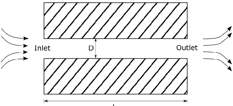
The experiments of Jinliang et al. (1995) are considered first. The experiments involved two-phase critical releases of pressurised water in sharp-edged tubes. The channel connecting the high and low-pressure domains has length 𝐿 = 4.0 𝑚𝑚 and diameter 𝐷 = 4.05 𝑚𝑚. Initially the pressure is kept constant at 40 bar and tests with different subcooling degrees are performed. The outlet pressure is 6.84 bar. An axisymmetric representation of the flow domain was used, using unstructured quadrilateral meshes of 24000 cells. The shape of the domain is shown in Fig. 1. Finer and coarser meshes with 60000 and 120000 cells were also used and results were found to be insensitive to grid resolutions.
Fig 1: Schematic of the flow domain for the experiments of Jinliang et al. (1995)
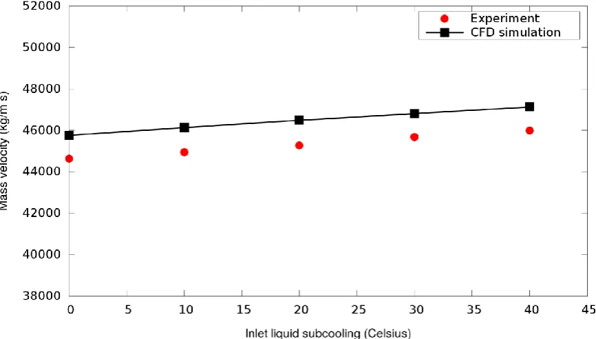
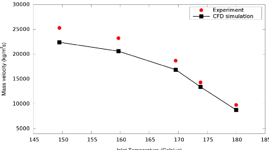
Results for the calculated mass flow rates per area a.k.a. mass velocity are shown in Fig. 2. The mass flux is not derived from an explicit formulation: instead, it is given as the product of the mass-averaged velocity with the mixture density. The simulations are from the case of subcooling of 40℃ up to the superheated case. In the latter case, the mass flux becomes minimum in both experiments and simulations and the results are in good agreement with the data with a difference less than 5%. An instantaneous axisymmetric contour of the density and void fraction is shown in Fig. 3 for the case of zero subcooling. It is evident that the vapour generation begins at the nozzle inlet, right after the geometry changes. This vapour annulus surrounding the liquid core is also reported for cases of low
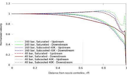
[image:11.595.104.491.258.434.2]characteristic parabolic velocity profile, common in single phase flows, is encountered here. At the centre of the pipe (r/R = 0) the velocity has its maximum value. Moving towards the nozzle walls, the axial velocity gradually decreases reaching its minimum at the wall boundary. Since the pressure drops along the axial direction, the downstream velocities are higher than the upstream with a ratio upstream-to-downstream velocity equal to approximatelely 0.63. The observations stand both for the subcooled and saturated flows, where velocity slightly changes. The peaks in the upstream velocities arise naturally due to the initiated cavitation caused by the flow separation shear layer at the low pressure area near the nozzle entrance.
Fig. 2: The predicted mass flow rates per area for initial pressure equal to 40 bar compared to experimental data of Jinliang et al. (1995).
[image:12.595.80.513.190.436.2] [image:12.595.83.509.482.646.2]
Fig. 4:The predicted mass flow rates per unit area for initial pressure equal to 160 bar compared to experimental data of Jinliang et al. (1995).
Fig. 5: The predicted velocities for different inlet pressures and temperatures upstream-downstream the nozzle.
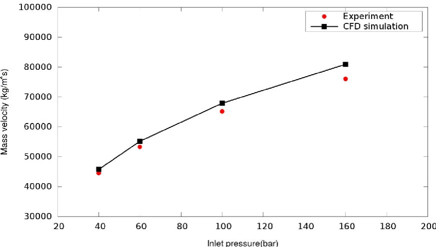
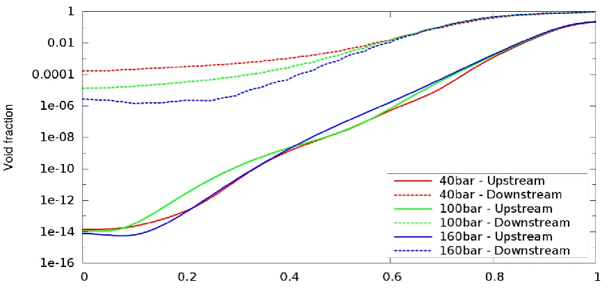
[image:13.595.79.510.383.640.2]jet at the end of the nozzle. The flashing inception is triggered when the jet pressure drops below the local saturation pressure. As mentioned in the experimental work used here for validation, the metastability of the flow starts at this point. The exact point where the flashing starts is non-trivial to determine, and there is no general model to predict it in the literature without limiting assumptions. The results are in good agreement, with a CFD-to-experiment difference generally less than 7%. The calculated void fraction is shown in Fig. 7. The void fraction is smaller in the centreline but increases closer to the wall as the result of the flow separation at the nozzle inlet. A qualitative perspective can be obtained from the void fraction, the pattern of which is more likely to change with increasing the ratio L/D as will be illustrated later. In all cases, the void fraction growth can be divided into three regions with respect to the distance from the centreline of the nozzle: from 0 to r/R equal to 0.15 it is almost constant, then increases on a log scale and from r/R between 0.8 and 1R grows fast to values that were usually around 0.45 in the nozzle inlet and close to the limit of unity at the nozzle end.
Fig. 6: The predictedmass flow rates per area for saturated stagnation conditions and different initial pressures up to 160 bar compared to experimental data of Jinliang et al. (1995).
Fig. 7: The predicted void fraction in logarithmic scale for the upstream and downstream positions of the nozzle and various inlet pressures of initially saturated conditions.
3.2 Turbulence and geometry impact on jet hydrodynamics
The ratio of the nozzle length to diameter may also play a crucial role in the flashing affecting bubble nucleation and atomisation. There are no strict limits as to whether the flow will exihibit internal or external flashing mode. Following Witlox’s (2002) review for flashing releases, one should expect the internal mode to be more likely to occur inside large nozzles although there is an uncertainty for short tubes. For nozzles with small 𝐿/𝐷 tested here, internal flashing occurs as well. The methodology developed in this study takes into account different parameters that could influence the correct mass flow rate calculation such as the compressibility and turbulence effects.
Pressure gradients are always present during liquid flow through the pipe, which cannot be a-priori estimated. A small pressure gradient may play a significant role in the momentum transport. Radial pressure gradients in turbulent pipe flows have been previously reported and seen that are an increasing function of Reynolds number. According to Iciek (1982) for long sharp-edged orifices of
𝐿/𝐷 > 5 turbulence is expected to be generated before the nozzle exit. On the other hand, for smaller
𝐿/𝐷 ratios, the inertial forces are likely to dominate viscous forces. A transition from laminar to turbulent regime is possible to occur in these cases, exhibiting a larger effect of 𝐿/𝐷 on the flow regime.
[image:15.595.77.515.75.285.2]this case the evaporation rate has more impact on the critical mass flow rate, hence a steeper mass flow rate curve.
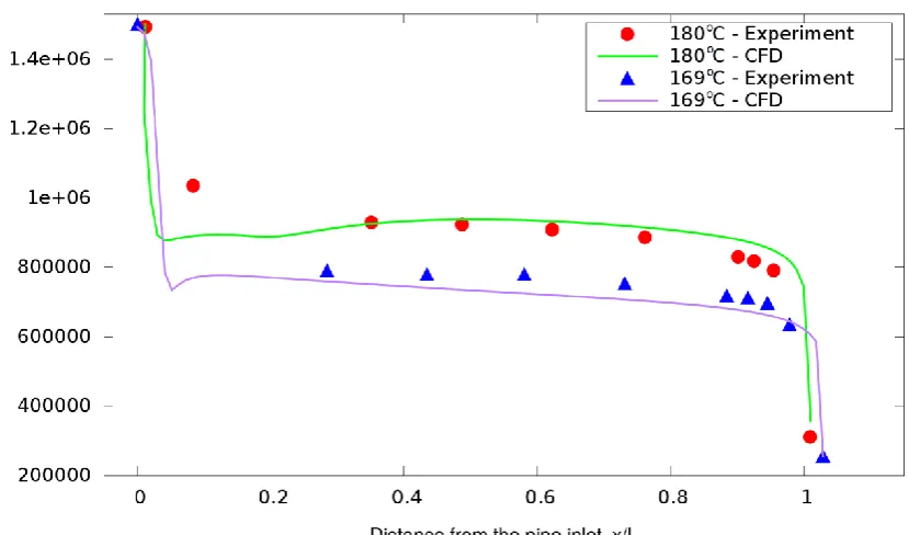
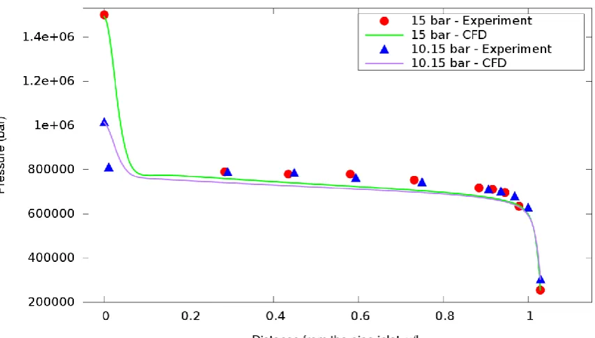
The pressure distribution within the pipe has also been studied. In flashing cases, the pressure drop is expected to be high and can be close to 50% of the initial storage pressure (Jinliang et al. 1995). In Fig. 9 the predicted pressure across the pipe is shown for two different initial temperatures. The first case is for the saturated state and the second one for a subcooling degree equal to 11 ℃. The stagnation pressure for both cases is 15 bar. In both cases, the same pattern is observed, which is the rapid pressure drop in the sharp inlet corner where the flow separates, and phase change starts. It is worth mentioning that the pressure at that point is, in both the experimental and numerical study, above the local saturation which implies that flashing is triggered downstream of the corner. Another interesting finding providing newer insights is that the pressure drop is generally higher in the subcooled case, meaning that the pressure along the pipe is more likely to be higher compared to the saturated inlet for the same initial pressure. The pressure difference in the case of subcooling degree of 11 ℃ is approximately one bar within the pipe up to the position which corresponds to the 85% of the pipe length, L.
[image:16.595.76.513.469.713.2]The relationship of pressure distribution with respect to the stagnation pressure of the liquid is investigated next. In Fig. 10 the cases of inlet pressures of 15 bar and 10.15 bar are compared for the case of initially subcooled water at 169 ℃. Surprisingly, the pressure drop downstream the inlet corner is the same in both cases, and the pressure profile is almost the same after the position of 5% of the pipe length. This can be interpreted that the pressure distribution within the nozzle is more sensitive in the subcooling degree than the initial pressure at the inlet, at least for nozzles with the relatively large length-to-diameter ratio. Increasing the L/D ratio, the mixture has more time to fully develop inside the nozzle. The effects of turbulent mixing become more importnant and the change in flow regime from pure liquid to bubbly is enhanced. Testing the water jet at 15 bar of Park et al. keeping the same diameter but for L/D equal to one, an indication for the L/D impact on the regime can be obtained. In Fig. 11 the void fraction for both cases has a similar trend with a larger minimum value and almost double for L/D = 29.4. Results of Fig. 7 demonstrate a smaller void fraction at the centreline for larger pressures with the one at 40 bar to be 104 times smaller. Nevertheless the diameter in Fig. 11 was 3.4 mm and not the same as in the case illustrated in Fig. 7 (D = 4 mm).
Fig. 10: The predicted pressure distribution inside the pipe for 169.4 oC and different initial pressures.
Fig. 11: The predicted void fraction for inlet pressure equal to 15 bar and different L/D for water flow.
3.3 Flashing in cryogenic liquids
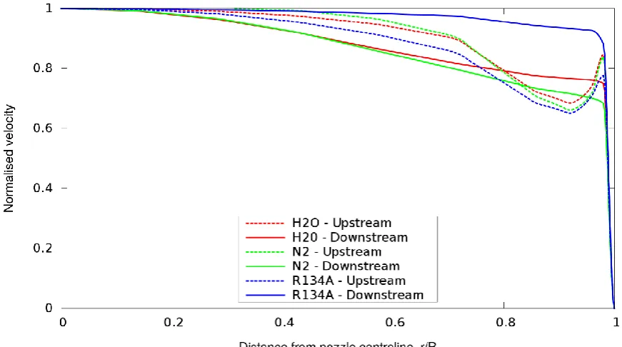
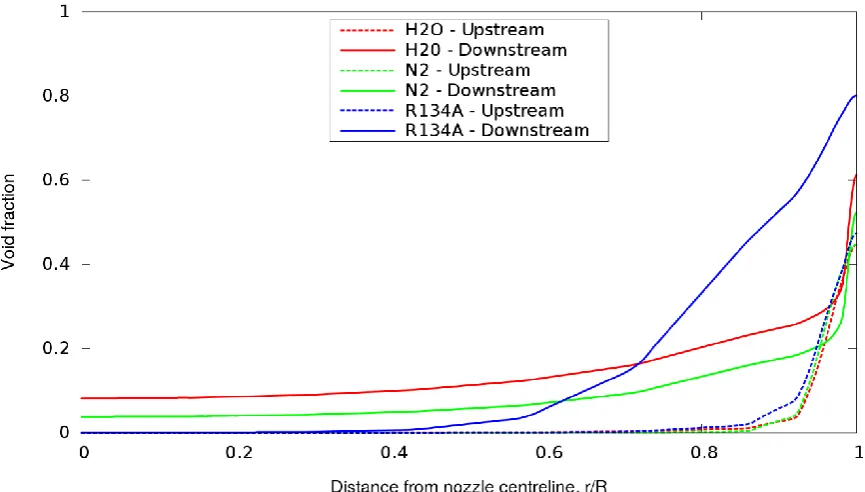
velocity at the upstream and downstream positions presented in Fig. 12 is divided by the maximum one for simplicity and plotted with respect to the whole nozzle diameter (r/R = 0 denotes the centre of the circular profile). The axial velocity is smooth close to the position of the maximum velocity at r/R = 0 but gradually changes when moving closer to the walls. The change in the velocity gradient occurs at almost the same distance for all the liquids at the downstream position. In the upstream case, the velocity profile becomes non-monotonic a bit further away from the wall and the velocity profile follows the patterns shown in Fig. 5. The same patterns appear in Winkhofer et al. (2001) where the cavitation gas exists in the shear layer enhancing the velocity peak. It is interesting that the patterns in velocity within the nozzle are similar for cryogenic and non-cryogenic fluid. The void fraction is expected to have its maximum in the recirculation zone close to the wall and becomes minimum at the centreline. Fig. 13 shows this trend for the void fraction. The centreline void fraction can vary in the position r/R = 0 and the difference in the volume occupied by the vapour is more extensive for the three liquids at the nozzle exit with a correspondingly different regime. One of the advantages of the presented methodology is that it can offer an estimation for the thickness of the vapour layer formed in the walls.
Fig. 13: Void fraction versus the distance from the centreline for the three liquids.
Conclusions
FlashFOAM, a new compressible solver has been developed within the frame of open source CFD code OpenFOAM to compute phase change within various nozzle and orifice geometries experiencing rapid pressure drops. FlashFOAM is capable of simulating flashing and the impact of bubble nucleation on the flow, and is validated using experiments with both subcooled and saturated initial conditions. The mass flow rates at the validated cases are close to those observed in the experiments. The predictions confirmed experimental findings that indicate a two-phase jet at the nozzle exit which continues evaporating downstream. The void fraction trends show an annular flow regime. In the presented method the liquid phase is tracked, and uses a novel pressure update. This pressure correction which is in the heart of the PIMPLE algorithm includes the effects of flash-boiling, ambient air entrainment and interfacial forces in a new numerical approach. Turbulence modelling is found to play a major role for accurate predictions of the mass flow rates and the 𝑘 − 𝜀 model appears to be adequate for the geometries presented. The model has been tested within the RANS framework but it can be implemented in the Large Eddy Simulations (LES) context as well to give more accurate predictions of primary atomisation. Models for the spray dynamics can be easily implemented and together with the VOF method the methodology presented can be used to derive a unified methology to simulate the whole process of liquid atomisation starting from inside the nozzle until the jet shatters to small droplets.
introduced to the problem. The current work needs to be extended to include the effects of the sub-grid scale turbulence for resolving more accurately the bubble dispersion patterns in the flow.
Acknowledgements
The authors wish to thank the Marie Curie Action of the 7th Framework Programme of the
European Union. The current work is part of the SafeLNG project (Project ID: 606754)
regarding the Numerical characterization and simulation of the complex physics
underpinning the Safe Handling of Liquefied Natural Gas (2014-2017).
References
Bianchi, G. M., Forte, C., Negro, S. and Pelloni, P., 2008.A 1d Model for the Prediction of Flash Atomization in GDI Multi-Hole Injectors: Preliminary Results. SAE Technical Paper Series, no. 2008-01-2516..
Bilicki, Z, and Kestin, J., 1990. Physical aspects of the relaxation model in two¬phase flow. Proceedings of the Royal Society of London. Series A, Mathematical and Physical Sciences, 379-397. Brackbill, J.U., Kothe, D.B., Zemach, C., 1992. A continuum method for modelling surface tension. J. Comput. Phys. 100, 335-354.
Downar-Zapolski, P., Bilicki, Z., Bolle, L. and Franco, J., 1996. The Non-Equilibrium Relaxation Model for one-dimensional Flashing Liquid flow. International Journal of Multiphase Flow 22,3, 473-483.
Einstein, A., 1920.Uber Schallschwingungen in teilweise dissoziierten Gasen. Sitzung Berl. Akad. Physik Chemie, 380-385
Fauske, H.K., 1962. Contribution to the Theory of Two-Phase. One Component Critical Flow. Argonne Natl. Lab. Tech. Report ANL-6633.
Fujimoto, H., Nishikori, T., Hojyo, Y., Tsukamoto, T., and Senda, J., 1994. Modelling of Atomisation and Vaporisation Process in Flash Boiling Spray. The International Conference on Liquid Atomisation and Spray Systems, Paper VI-13, Rouen.
Henry, RE., 1970.The two-phase critical discharge of initially saturated or subcooled liquid. Nuclear Science Engineering41 336–342.
Iciek, J., 1982. The hydrodynamics of a free, liquid jet and their influence on direct contact heat transfer - I and II. Int. J. Multiphase Flow 8 3, 239–260.
Ishimoto, J., Ohira, K., Okabayashi, K. and Chitose, K., 2009. Integrated Numerical Prediction of Atomization Process of Liquid Hydrogen Jet. J. Cryo. Soc. Jpn. 44, 7.
Issa, R.I., 1986. Solution of the implicitly discretised fluid flow equations by operator-splitting. J. Comput. Phys. 62, 40–65.
Jasak, H., 1996. Error Analysis and Estimation for the Finite Volume Method with Applications to Fluid Flows, Ph.D Thesis, Imperial College of Science, Technology and Medicine, London.
Jiang, X., Siamas, G.A., Jagus, K., Karayiannis, T.G., 2010. Physical modelling and advanced simulations of gas liquid two-phase jet flows in atomization and sprays. Progress in Energy and Combustion Science 36 131-167.
Jinliang, Xu, Tingkuan, Chen, T., Yang, L., 1995. Two-Phase Critical Discharge of Initially Saturated or Subcooled Water Flowing in Sharp-Edged Tubes at High Pressure. J. of Thermal Science 4, 3, 193-199.
Lee, .J, Madabhushi, R., Fotache, C., Gopalakrishnan, S., Schmidt, D., 2009. Flashing flow of superheated jet fuel. Proceedings of the Combustion Institute 32 3215–3222.
Yixiang, Liao, Lucas, Dirk, 2015. 3D CFD simulation of flashing flows in a converging-diverging nozzle, Nuclear Engineering and Design 292 149–163.
Moody, F.J., 1965. Maximum Flow Rate of a Single Component, Two-Phase Mixture. J. Hear Transfer 87 134- 141.
Menter, F.R., 1993. Zonal Two Equation k-ω Turbulence Models for Aerodynamic Flows. AIAA Paper 93-2906.
Oza, R.D., and Sinnamon, J.F., 1983. An experimental and analytical study of flash boiling fuel injection. SAE Paper 830590.
Park, B.S. and Lee, S.Y., 1994. An Experimental Investigation of the Flash Atomisation Mechanism. Atomisation and Sprays, 4 159-179.
Patankar, S. V., 1980. Numerical Heat Transfer and Fluid Flow. Hemisphere Publishing Corporation, New York.
Park, C-K, Park, J-W, Chung, M-K, and Chung, M-H., 1997. An empirical correlation for the Critical Flow Rates of Subcooled Water Through Short Pipes with Small Diameters. Journal of the Korean Nuclear Society, 29 1, 35-44, 1997.
Poinsot, T.J., and Lele, S.K., 1992. Boundary Conditions for Direct Simulations of Compressible Viscous Reacting Flows. Journal of Computational Physics, 101, 104-129.
Prosperetti, A., Tryggvason, G., 2006. Computational Methods for Multiphase Flow, Cambridge University Press.
Reinke, P., Yadigaroglu, G., 2001. Explosive vaporisation of superheated liquids by boiling fronts. Int. J. Multiphase Flow, 27, 1487-1516.
Rusche, H., 2002. Computational fluid dynamics of dispersed two-phase flows at high phase fractions. PhD thesis, Imperial College London.
Salvador, F. J, Jaramilloa, D., Romero, J.V., Roselló, M.D., 2017. Using a homogeneous equilibrium model for the study of the inner nozzle flow and cavitation pattern in convergent–divergent nozzles of diesel injectors. Journal of Computational and Applied Mathematics 309, 630–641.
Schmidt, D.P, Gopalakrishnan, S., Jasak, H., 2010. Multi-dimensional simulation of thermal non-equilibrium channel flow. International Journal of Multiphase Flow 36, 284–292.
Schroder, Jens Jurgen, and Nha, Vuxuan, 1987. Homogeneous Non-Equilibrium Two-Phase Critical Flow Model. Chem. Eng. Technol. 10, 420-426.
Sher, Eran, Tali, Bar-Kohany, Rashkovan, Alexander, 2008. Flash –boiling atomization. Progress in Energy and Combustion Science 34, 417-439.
Srinivasan, V., Salazar A., Sait, K., 2010. Modeling the disintegration of cavitating turbulent liquid jets using a novel VOF–CIMD approach. Chemical Engineering Science 65, 2782–2796.
Wareing, Christofer J., Fairweather, Michael, Falle, Samuel, A.E.G., Woolley, Robert, M., 2014. Validation of a model of gas and dense phase CO2 jet releases for carbon capture and storage application. International Journal of Greenhouse Gas Control 20, 254–271.
Weller, Henry, Tabor, G., Hrvoje, Jasak, Fureby, C., 1998. A tensorial approach to computational continuum mechanics using object-oriented techniques. Comput. Phys. 12, 620–631.
Wen, Jennifer, Heidari, Ali, Xu, Baopeng and Jie, Hongen, 2013. Dispersion of carbon dioxide from vertical vent and horizontal releases-A numerical study. Proc IMech Part E: J Process Mechanical Engineering 227 2, 125-139.
Wen, Jennifer, X, Le Fur, Pierre, Jie, Hongen, and Vendra, C. Madhav, Rao, Further development and validation of CO2FOAM for the atmospheric dispersion of accidental releases from carbon dioxide
pipelines, International Journal of Greenhouse Gas Control, Volume 52, September 2016, Pages 293-304.
Winklhofer, E., Kull, E., Kelz, E., and Morozov, A., 2001. Comprehensive hydraulic and flowfield documentation in model throttle experiments under cavitation conditions. ILASS Europe.
Witlox, H., Bowen, P.J,. 2002. Flashing liquid jets and two-phase dispersion A review. Contract research report 403/2002, HSE.