Value of information methods to design a clinical trial in a small population to optimise a health economic utility function

warwick.ac.uk/lib-publications

Original citation:

Pearce, Michael, Hee, Siew Wan, Madan, Jason, Posch, Martin, Day, Simon, Miller,

Frank, Zohar, Sarah and Stallard, Nigel (2018) Value of information methods to design a

clinical trial in a small population to optimise a health economic utility function. BMC

Medical Research Methodology, 18 (1). p. 20. doi:

10.1186/s12874-018-0475-0

Permanent WRAP URL:

http://wrap.warwick.ac.uk/99080

Copyright and reuse:

The Warwick Research Archive Portal (WRAP) makes this work of researchers of the

University of Warwick available open access under the following conditions.

This article is made available under the Creative Commons Attribution 4.0 International

license (CC BY 4.0) and may be reused according to the conditions of the license. For more

details see:

http://creativecommons.org/licenses/by/4.0/

A note on versions:

The version presented in WRAP is the published version, or, version of record, and may be

cited as it appears here.

R E S E A R C H A R T I C L E

Open Access

Value of information methods to design a

clinical trial in a small population to optimise a

health economic utility function

Michael Pearce

, Siew Wan Hee

, Jason Madan

, Martin Posch

, Simon Day

, Frank Miller

, Sarah Zohar

and Nigel Stallard

Abstract

Background: Most confirmatory randomised controlled clinical trials (RCTs) are designed with specified power, usually 80% or 90%, for a hypothesis test conducted at a given significance level, usually 2.5% for a one-sided test. Approval of the experimental treatment by regulatory agencies is then based on the result of such a significance test with other information to balance the risk of adverse events against the benefit of the treatment to future patients. In the setting of a rare disease, recruiting sufficient patients to achieve conventional error rates for clinically reasonable effect sizes may be infeasible, suggesting that the decision-making process should reflect the size of the target population.

Methods: We considered the use of a decision-theoretic value of information (VOI) method to obtain the optimal sample size and significance level for confirmatory RCTs in a range of settings. We assume the decision maker represents society. For simplicity we assume the primary endpoint to be normally distributed with unknown mean following some normal prior distribution representing information on the anticipated effectiveness of the therapy available before the trial. The method is illustrated by an application in an RCT in haemophilia A. We explicitly specify the utility in terms of improvement in primary outcome and compare this with the costs of treating patients, both financial and in terms of potential harm, during the trial and in the future.

Results: The optimal sample size for the clinical trial decreases as the size of the population decreases. For non-zero cost of treating future patients, either monetary or in terms of potential harmful effects, stronger evidence is required for approval as the population size increases, though this is not the case if the costs of treating future patients are ignored.

Conclusions: Decision-theoretic VOI methods offer a flexible approach with both type I error rate and power (or equivalently trial sample size) depending on the size of the future population for whom the treatment under investigation is intended. This might be particularly suitable for small populations when there is considerable information about the patient population.

Keywords: Decision theory, Health economics, Power, Rare disease, Regulator, Type I error, Value of information

*Correspondence:[email protected]

2_{Statistics and Epidemiology, Division of Health Sciences, Warwick Medical}

School, University of Warwick, Coventry, UK

Full list of author information is available at the end of the article

Pearceet al. BMC Medical Research Methodology (2018) 18:20 Page 2 of 9

Background

Prior to approval a drug typically goes through various phases of clinical development, beginning with assess-ing pharmacology in humans (phase I), followed by exploration of therapeutic efficacy (phase II) and finally, confirmation of the effectiveness (phase III). This is not a necessary ordering, for example, prior to presenting over-all clinical development, results and issues of the drug’s efficacy and safety (this list is long) to regulatory agencies, further investigation of the effect on human pharmacol-ogy may be conducted. Based on the submitted informa-tion, the regulatory authorities approve the product that has demonstrated safety and effectiveness for the intended population.

Treatments for rare diseases may not go through all the phases of clinical development prior to submission to reg-ulatory authorities. Buckley presented a brief summary of treatments intended for rare diseases and approved by European regulator that did not go through all these phases [1]. The difference is usually attributable to the small population where it is infeasible or impossible to recruit many patients for trials.

The focus of this paper is the design of phase III trials in particular in a small population. One of the fundamental issues in clinical trial design is sample size determination. The most common approach is to perform a power cal-culation for a hypothesis test. In a two-arm randomised controlled trial aiming to establish superiority of an exper-imental treatment to the standard treatment, the null hypothesis may state that the experimental treatment is not superior to the control.

The sample size is determined by restricting type I and II error rates. A type I error occurs when a true null hypothesis is rejected and a type II error occurs when a false null hypothesis is not rejected. Typically, the one-sided type I error rate,α, is set to 0.025. The type II error rate,β, is set to 0.10 or 0.20 for some specified alternative hypothesis. Correspondingly, the power to detect the pre-defined value, 1−β, is 0.90 or 0.80. Values forα andβ are customarily set without consideration of the severity or prevalence of the disease. In practice, however, clinical trials in rare diseases have smaller sample sizes than those in more common conditions, indicating that conventional type I and type II error rates are being compromised in this setting [2,3]. Increasing the type I error rate might be appropriate in a trial for rare disease as the small popula-tion means that the number of patients who would benefit from an effective treatment may be small and so it may be justifiable to have alternate levels of type I error so that an effective treatment may be made available more easily.

To determine the sample size it seems reasonable to consider information such as previous trial outcomes, the cost of making type I or type II errors, the number of

people affected, the financial burden of the treatment and other costs and rewards that will result from the treatment being approved and marketed . One model that could be used to optimise the sample size accounting for all the information is the Bayesian decision theoretic approach. In this framework, decisions are made so as to maximise a utility function that quantifies their desirability of an out-come. The utility function may be made up of observed responses from a sample of patients, the costs of treat-ing patients and conducttreat-ing the trial, and the profits from a successful treatment. Some authors have proposed to include the cost of trials, the profit from a successful trial (or a loss from an unsuccessful trial), two endpoints (e.g. efficacy and adverse events) and the size of the popula-tion, N, so that the sample size required for the trial is optimised (see Hee et al. [4]). By including N we also incorporate the potential gain to future patients. Such an approach seems particularly suitable in the setting of a small population, when there is likely to be considerable knowledge of the size of the target population prior to the start of a clinical trial and this is likely to be much smaller than in other settings.

Methods

A Bayesian decision theoretic approach to sample size determination

In our approach we assume that following safety and effi-cacy exploration studies, once the drug has been shown to be effective in a phase III trial for the intended pop-ulation, it obtains regulatory approval. The objective of a phase III trial is primarily to confirm effectiveness. The typical design considered to be the gold standard in providing the best evidence in assessing efficacy is the randomised controlled trial (RCT). Let n be the size of the RCT and assume that patients are randomised in a 1:1 ratio to either the experimental or standard arm. Let Yi = (Yi1,. . .,Yin/2), i = (E,S), denote the

out-comes andY¯idenote the sample mean fromn/2 patients

from the experimental (E) and standard treatment (S) arms, respectively. Assume Y¯i is normally distributed

with mean θi and known variance, 2σi2/n, that isY¯i ∼

Nθi, 2σi2/n

. In the classical frequentist setting, we test the null hypothesis that the two population means,θEand

θS, are equal, equivalently θ = θE −θS = 0. The

dif-ference of the sample means, denoted by X¯ = ¯YE − ¯YS

is normally distributed with mean θ and variance τ2/n

where τ2/n = 4σ2/n when σ_E2 = σ_S2 = σ2 (equal variance) or τ2/n = 2σ_E2+σ_S2/n when σ_E2 = σ_S2 (unequal variance).

In the Bayesian setting, θ is assumed to be unknown but to follow a distribution with specified form. Assume that the prior density of θ, which measures the belief regarding the parameter prior to observing any responses, is Nμ0,σ₀2

previous trials, case studies or experts’ opinions [5–9]. Following observations from patients, the prior is updated to give a posterior distribution summarising belief about

θgiven the observed data.

In the Bayesian decision theoretic framework, a util-ity function summarises the value of all possible actions givenθ. The action that maximises the expectated value of this utility over the posterior distribution of θ given the observed data can then be chosen as the optimal action. As with frequentist hypothesis testing, we may consider that at the end of the trial, there are two possi-ble actions, to reject the null hypothesis or not. The utility function depends on the sample sizen, and the decision,

d ∈ {do not reject H0, reject H0}, given θ. Let d(x¯,n)

denote the action taken at the end of the trial given data

¯

x with a sample size n andG(n,d,θ) denote the utility function. We may also choosenoptimally. As we will not have observed any responses during the planning stage, the expected utility is obtained from the distribution ofX¯

givenθ andn. Asθ is unknown, the expectation of the expected utility is taken over the prior density [4]. The expected utility is then a function of the sample size and decision rule, denoted by

G(n,d)=

¯

x

G(n,d(x¯,n),θ)f(θ|¯x,n)dθf(x¯|n)dx¯,

(1)

wheref(θ|¯x,n)is the posterior density ofθgivenx¯and

f(x¯|n)= 1

σxφ

_¯

x−μ0 σx

is the prior-predictive density function forX¯ before sam-pling, withσ2

x = σ02+τ2/nthe prior predictive variance

ofX¯ andφ(·)the normal density function. If the action taken at the end of the trial is determined by the out-come of some hypothesis test, the functiondand hence the expected utilityG(n,d), will depend on the type I error rate, or equivalently the critical value, for that test, as described in more detail in the next subsection. The opti-misation problem then becomes one of choosing the trial sample size and test type I error rate.

Formulation of utility function

We assume that the decision maker for our proposed model represents society. A reward corresponds to improved treatment either of patients in the trial or of future patients if the experimental treatment receives reg-ulatory approval.

The regulator is assumed to approve the experimental treatment if the observed difference,X¯ = ¯x, is greater than a threshold,z_ατ/√n, wherez_αis the upperαpercentile of the standard normal distribution, so thatd(x¯,n)=‘reject

H0’ or ‘do not rejectH0’ forx¯above or below this

thresh-old. This is equivalent to a classical frequentist analysis of the primary endpoint using a significance test con-ducted at (one-sided) levelα. This assumption is similar to that proposed by Pezeshk et al. who also assume that the regulatory agency will test the null hypothesis that there is no difference between the outcomes means at the α test size [10]. Since the decision function d then depends only on zα, we will write G(n,zα) for G(n,d)

given by (1) above, and refer tozαas the significance level threshold.

We assume that the size of the population for the treat-ments we are testing is known, and denote this by N. The number of patients that can be treated following the trial depends onN and on the trial sample size. We assume that during the trial a proportionρof patients are enrolled in the trial, so that there aren(1−ρ)/ρ concur-rent patients not enrolled in the trial and the number of patients remaining to be treated isN−n/ρ.

We suppose that the utility givenx¯ represents the gain from treating patients with the experimental treatment. There aren/2 such patients in the trial and, ifx¯≥zατ/√n

so that the new treatment is approved, N − n/ρ such patients following the trial. The reward for each treated patient is taken proportional to the true effect size, i.e. the more effective the treatment is the greater the reward will be. Note that it is considered a loss if the treatment effect is<0.

The utility function also includes fixed and variable financial costs [11]. Fixed costs are incurred regardless of the size of the trial, denoted bycf; these may be the

set-ting up and running cost of the trial. Variable costs depend on the size of the trial. The cost per patient, denoted by

c1, may be administrative costs to recruit, screen, treat

and follow-up patients in the conduct of the trial. Our proposed utility function also includes additional costs, either monetary or harmful effects, of treating a patient with the experimental treatment, denoted byc2. All these

costs may be scaled to one unit of efficacy such that they are relative toθ. Alternatively, the treatment efficacy may be scaled to one unit of cost such that it is relative to monetary reward and costs [12].

Pearceet al. BMC Medical Research Methodology (2018) 18:20 Page 4 of 9

G(n,d,θ)=

⎧ ⎪ ⎪ ⎪ ⎨ ⎪ ⎪ ⎪ ⎩

(θ−c2)

N−_ρn+ n₂−c1n −cfI{n>0} d=rejectH0, (θ−c2)n₂−c1n

−cfI{n>0} d=do not rejectH0,

(2)

whereI{n>0} =1 ifn> 0 and 0 otherwise. The expected utility given by (1) is then

G(n,zα)

= (N−n/ρ)(θ−c2)I{¯x≥zατ/√n}

+n

2(θ−c2)−c1n−cfI{n>0}

×f(θ|¯x)f(x¯|n)dθdx¯

=(N−n/ρ)

(μ0−c2)(−Z)+ σ 2 0 σxφ(

Z)

+n

2(μ0−c2)−c1n−cfI{n>0},

(3)

where (·) is the normal cumulative distribution func-tion and Z = (zατ/√n− μ0)/σx is the z-score of the

significance level threshold, zα, on the prior predictive distribution of X¯. The full derivation is presented in the Additional file1.

Optimisation

The optimal sample size and significance level threshold are obtained by maximising the expected utility,G(n,zα). Letz∗_α denote the optimal value for the significance level threshold. This is obtained for any n by differentiating

G(n,z_α)with respect toz_α, to obtain

d

dzαG(n,zα)=(N−n/ρ)(μ0−c2)

d

dzα(−Z)

+(N−n/ρ)σ 2 0 σx

d dzαφ(Z)

=(N−n/ρ)

(μ0−c2)τ/ √

n

σx φ(

Z)

+σ02 σx

τzατ/√n−μ0

/√n

σ2

x

φ(Z)

. (4)

Equating the differentiated expression (4) to zero, for a given sample sizenthe optimalz_αis

z∗_α=c2σ 2 x √ n σ2 0τ

−μ0 τ

σ2 0 √

n. (5)

Subsequently, the optimal sample size, n∗, is obtained numerically by substituting (5) into (3) (see Additional file1for details).

Results

Application to a case study

Abrahamyan et al. presented a decision analytic value of information (VOI) model for assessing evidence on treat-ments for children with severe haemophilia A, a rare dis-ease [12]. They summarised that there are three types of treatments currently available in various developed coun-tries; alternate day prophylaxis (AP), on-demand (OD) and tailored prophylaxis (TP) of intravenous administra-tion of recombinant Factor VIII (FVIII). They utilised information from US and Canada studies to evaluate whether or not to conduct another trial. They performed three pairwise comparisons; TP vs. AP, OD vs. TP and OD vs. AP, and in each comparison the optimal decision, whether to conduct another trial or to accept one of the treatments as a standard therapy, was given depending on the maximum acceptable price per unit health gain.

We adapted this work to illustrate the application of our proposed model. Table 1 shows the estimated val-ues used in our example. The primary endpoint was binary, whether or not the patient had magnetic reso-nance imaging (MRI)-detected joint damage. Similar to Abrahamyan et al., we assume large sample approxima-tions to this binary endpoint and so the efficacy mean,

ˆ

μt,t = (AP, OD, TP), is the proportion of patients

with-out MRI-detected joint damage. The sample and prior variances areσˆ_t2= ˆμt(1− ˆμt)andσˆ₀2_t=var(μˆt)= ˆμt(1−

ˆ

μt)/n0t, respectively where n0t is the number of prior

observations for treatmenttreported by Abrahamyan et al., that isn0,AP=27,n0,OD=29 andn0,TP=24.

To illustrate our model, consider a two-arm RCT com-paring the on-demand (OD), which we assumed to be the standard treatment, with the tailored prophylaxis (TP). The point prevalence of haemophilia A in US is 7.0 per 100,000 which is about 22,400 in the US given the US population of approximately 320 million [13,14].

Let the measure of efficacy be the absence of MRI-detected haemophiliac joint damage and the unknown parameter measuring treatment benefit be the differ-ence of proportion of patients without MRI-detected joint damage valued in monetary terms using the value the decision-maker places on each unity of efficacy, which will be denotedλ. The prior distribution for the unknown

Table 1Summary statistics and costs (in dollar, $) by treatment for haemophilia A, adapted from Abrahamyan et al. [12]

Treatment,t

Statistics AP OD TP

Prior mean,μˆt 0.9259 0.5517 0.7917

Prior variance,σˆ2

0t 0.0025 0.0085 0.0069

Sample variance,σˆ2

t 0.0686 0.2473 0.1649

Mean cost,c2t($) 176,397 56,619 117,651

parameter is then normal with prior meanμ0=λ(μTP− μOD) and prior variance σ02 = λ2

σ2

0,TP+σ0,OD2

. As

shown in Table1,σ_TP2 =σ_OD2 , therefore, the sample vari-ance is estimated by τ2 = 2λ2σ_TP2 +σ_OD2 . Following Abrahamyan et al., take λ = $400, 000 leading to the values given in Table2. Suppose the fixed financial cost incurred from conducting the trial isc_f = $1m, the cost of conducting the trial per patient isc1=$5, 000 and the

cost of treating a patient isc2= c2,TP−c2,OD= $61, 032

(see, Table2).

Similar to Abrahamyan et al., we assume annual haemophilia A incidence of 200 with 1/5 of patients recruited to the trial (ρ = 0.2). Let the time horizon be 20 years and assume that all new cases will be prescribed with the recommended treatment after the trial. The total number of future patients who will benefit from the new treatment is thus 4000−5n.

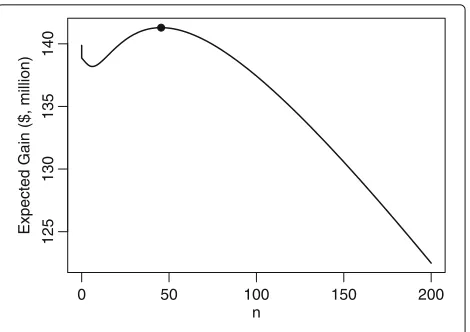
Figure1 shows the expected utility forzα = z∗_α for a range of values ofn. The optimal sample size, correspond-ing to the value for which the expected utility is highest is shown by the plotted point and is equal ton∗ = 46 (i.e. 23 patients per arm),Gn∗,z∗_α = $141 million and the threshold to approve TP isz∗_α = 0.36876, equivalent to

α=0.35615.

Bothn∗ andz_α∗ are far from their conventional values. In particular, except in the cases whenn=0, the power is much smaller than a conventional level. Takingα=0.025 andβ = 0.8 for an alternativeθA = σ0/2 = $24, 819

would requiren=268. The expected utility for this design is $109 million.

Operating Characteristics

Figure 2 shows optimal sample sizes and significance levels obtained from our model for population sizes between 100 and 10,000,000 with other parameters fixed asθ ∼ N96, 000,(49, 638)2_,τ2 _{= ($363, 202)}2_,c

1 =

$5, 000,c2=$61, 032 andcf =$1m. Figure2ashows that

if the population is small (N < 3000), the optimal sam-ple size isn∗ = 0. In this case the optimal significance level threshold to approve TP isz_α∗ → −∞(equivalently,

Table 2Parameter estimates for the pairwise comparison between on-demand (OD) and tailored prophylaxis (TP)

Parameter Estimates

Population size,N 4000

Prior mean,μ0=λ(μTP−μOD), ($) 96000

Prior variance,σ₀2=λ2σ_0,TP2 +σ_0,OD2 , ($) (49638)2

Sample variance,τ2_=2λ2_σ2

TP+σOD2

, ($) (363202)2

Cost of conducting the trial per patient,c1, ($) 5000

Cost of treating a patient,c2=c2,TP−c2,OD, ($) 61032

Fixed financial cost incurred from conducting the trial,cf, ($) 1 million

0 50 100 150 200

125

130

135

140

n

Expected Gain ($, million)

Fig. 1Expected utility,Gn,z_α∗, againstn

α→1, see Fig.2canddrespectively), corresponding to an optimal decision to approving the experimental treatment based on the prior belief alone.

Other than for very small population sizes (N >3, 000) the optimal trial sample size increases with N, with log(n∗) increasing approximately linearly with log(N). This reflects work by Cheng et al. and Stallard et al. show-ing that asN increasesn∗ ∝ √N [15,16]. The optimal significance level decreases as N increases (Fig. 2d), requiring a stricter level of statistical significance. Figure2bshows the type II error rate of the test using sam-ple size n∗and significance level threshold z∗_α, to detect an alternative θA = σ0/2 = $24, 819. In this case the

type II error rate increases to approach 1 asNincreases, so that that power approaches 0. This is reasonable since as θA < c2, this true effect difference is insufficient

to justify recommendation of the treatment for use in future patients, though is very different to a more con-ventional approach in which the power will increase with increasingn.

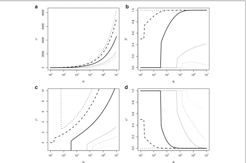
Figure3shows optimal sample size (n∗), thresholdz∗_α, type I (α∗), and II (β∗) error rates, against the size of the population for various values of cost, c2 = 0,c2 =

$12, 409,c2 = $24, 819,c2 = $61, 032,c2 = $96, 000 and c2=$120, 819. Cases includec2equal to, above and below θAand the prior mean.

Whenc2 = 0 we have n∗ > 0 only ifN > 390, 000

(Fig. 3a). If N < 390, 000 the optimal decision is to approve the experimental treatment without a trial. When

c2 = μ0, it is optimal not to start the trial if the

popu-lation size,N < 200. In this case prior belief is that the expected utility from the new and standard treatments are equal so that rejection or non-rejection ofH0lead to the

same expected utility sozα can be taken to be∞or−∞, or equivalentlyαmay be taken to be 1 or 0. Whenc2> μ0

Pearceet al. BMC Medical Research Methodology (2018) 18:20 Page 6 of 9

0

1000

2000

3000

4000

N

n*

102 ₁₀3 ₁₀4 ₁₀5 ₁₀6 ₁₀7

a

0.0

0.2

0.4

0.6

0.8

1.0

N

β

*

102 ₁₀3 ₁₀4 ₁₀5 ₁₀6 ₁₀7

b

02468

1

0

N

z*

102 ₁₀3 ₁₀4 ₁₀5 ₁₀6 ₁₀7

c

0.0

0.2

0.4

0.6

0.8

1.0

N

α

*

102 ₁₀3 ₁₀4 ₁₀5 ₁₀6 ₁₀7

d

Fig. 2Optimal (a) sample size,n∗, (b) type II error rate,_β∗, in order to detect an alternative_θA=σ0/2=$24819 (c)z∗_αand (d) type I error rate,α∗

against the size of the population,N, with fixed_μ0=$96000,σ02=($49638)2,τ2=($363202)2,c1=$5000,c2=$61032 andcf =$1 million

is shown in Fig.3d where the optimal type I error rate,

α∗ _{→ 0. The optimal type II error rate, β}∗ _approaches

1 (power approaches 0) asNandn∗become large when

c2 > θA and, though this is hard to see from the plot,

approaches 0 (power approaches 1) asN becomes large whenc2 < θA. Although not shown on these plots, asc2

becomes very large, the optimal sample size,n∗, decreases, with n∗ = 0 for largestc2 values reflecting very strong

prior belief that the TP is not sufficiently promising to overcome the costc2.

Additional calculations were performed to evaluate the sensitivity of the results obtained to specification of the prior mean,μ0, and variance,σ₀2. Figures illustrating

the optimal design parameters,n∗andα∗are given in the Additional file2. These show that increasing or decreasing

μ0has a similar effect on the choice ofnandαas

decreas-ing or increasdecreas-ingc2and that increasing or decreasing the

prior variance, that is decreasing or increasing the level of prior information assumed, decreases or increases the value ofNbelow whichn∗=0.

Discussion

The methodology of decision theory is the foundation of the value of information (VOI) method presented in the

0

2000

4000

6000

8000

N

n*

102 103 104 105 106 107

a

0.0

0.2

0.4

0.6

0.8

1.0

N

β

*

102 103 104 105 106 107

b

02468

1

0

N

z*

102 ₁₀3 ₁₀4 ₁₀5 ₁₀6 ₁₀7

c

0.0

0.2

0.4

0.6

0.8

1.0

N

α

*

102 ₁₀3 ₁₀4 ₁₀5 ₁₀6 ₁₀7

d

Fig. 3Optimal (a) sample size,n∗, (b) type II error rate,_β∗, (c)z∗_αand (d) type I error rate,_α∗in order to detect an alternative_θA=$24819 against

the size of the population,N, with fixed_μ0=$96000,σ02=($49638)2,τ2=($363202)2,c1=$5000 andcf=$1 million for different values of;

c2=0 (light grey dotted line),c2=σ0/4=$12409 (light grey dashed line),c2=σ0/2=$24819 (light grey solid line),c2=$61032 (heavy black

solid line),c2=μ0=$96000 (heavy black dashed line) andc2=σ0/2+μ0=$120819 (heavy black dotted line)

reflected in the construction of the utility function used, for example in the assumption of a fixed finite future pop-ulation, with this decreasing in size depending on the length of the clinical trial.

Regulatory agencies may prefer the use of classical frequentist methods in the evaluation of pharmaceuti-cal products. In the design of a clinipharmaceuti-cal trial based on the frequentist method, the type I error rate, α, is usu-ally restricted at a one-sided 0.025 level. This value is a conventional, but arbitrary, choice, and there is some indication that in practice there may be some flexibility depending on severity and/or prevalence of the disease. Our approach involves calculating a z-score for a pri-mary clinical outcome that corresponds to maximising expected utility. It therefore allows a hypothesis testing framework to be maintained, but ensures that the error rate for that hypothesis test on the primary outcome is consistent with a utility maximisation framework. Results from Fig.3suggest that differentα-levels are appropriate for diseases with different prevalence rates. Discussion of choice ofα-level depending on prevalence and severity of disease has been considered by Montazerhodjat and Lo

(2015) [17]. In their working paper they also show that the optimal critical value increases with disease preva-lence, but find a greater dependence on the severity of the disease with a more severe disease (e.g. pancre-atic cancer) requiring a lower critical value (e.g. zα =

0.587,α = 0.279) and a less severe disease (e.g. prostate cancer) requiring a higher critical value (e.g.zα = 2.252,

α=0.012).

In the example presented above, we made some simpli-fying assumptions from the Abrahamyan et al. model for tractability, such as assuming independence of costs and clinical outcomes, which lead to slightly different optimal designs. In our model, we assumed that there is a non-trial cost in treating a patient with the experimental treat-ment,c2, that is known and fixed. However,c2may also

Pearceet al. BMC Medical Research Methodology (2018) 18:20 Page 8 of 9

or observing adverse events both within and outside the trial which will affect costs and take-up of the new treat-ment [18–20]. As such the optimisation of sample size may depend on two endpoints; efficacy and safety. This may be simplified by aggregating efficacy and safety in a clinical utility index that could be used as the primary endpoint. Therefore, the unknown parameter, θ, would represent the mean difference in this utility index.

There are two possible decisions in our model where the experimental treatment is approved for treating future patients depending if the observed difference is greater than the optimal threshold. An alternative to defining the threshold at some frequentist test size, we could define it as some monetary value such as willingness to pay for one unit of health, e.g. in the model proposed by Willan and Eckermann where the decision making is from the perspective of the society who is responsible to decide whether or not to reimburse a new intervention at the given price to the company. In their model, the societal’s decision is based on the threshold of the willingness to pay at a certain price [21].

We also assume that the size of the population is known. Based on Abrahamyan et al., who estimated the annual incidence to be 200, we took N = 4000 correspond-ing to a 20 year period of market exclusivity (the time during which the new treatment is the sole drug in the market). Alternatively, the population size could be mod-elled by considering the accrual time, market exclusivity period (the new treatment being the sole drug in the market) and the delay taken from the availability of results to the submission to the regulatory approval, production, marketing, distribution and sales [11, 19, 21, 22]. The inclusion of time or a model of growth and decay in our model is straight forward.

The estimate of the proportion of patients who will benefit from the new treatment if it is approved for rou-tine use may be more complex by including patient’s life expectancy and quality of life [23–25]. Or depending on the severity of the disease, the number of future patients who would take up the recommended new treatment depends on the treatment efficacy in a piecewise linear function [10, 26–29]. There may be no future patients who receive the treatment if the effectiveness is lower than a predefined threshold and some maximum number of patients if it is greater than a predefined threshold, i.e. the improvement is sufficiently large. If the efficacy is in between the lower and upper thresholds, the number of patients is a linear function that increases with the effi-cacy. This could effectively limit the choice of the optimal value α∗ as insufficiently strong evidence from the trial of a treatment effect might lead to the new treatment not being used for any patients following the trial.

A challenge associated with implementation of the method proposed is specification of the prior distribution.

A number of authors have discussed elicitation of prior distribution parameters for Bayesian trial design, includ-ing in the settinclud-ing of a rare disease [9,30]. Using a more informative prior generally results in a smaller optimal trial sample size, sometimes with the optimum to be to conduct no trial at all but to make a decision based on prior data alone. If this is considered to be inappropriate, careful consideration should be given to the prior distribu-tion as well as the specificadistribu-tion of parameters of the utility function.

We have assumed that regulatory agencies make a simplistic binary decision, approve or not the submit-ted product. Agencies such as FDA/EMA may also give “accelerated approval/conditional approval”. Our pro-posed model can be expanded to include this decision where the utility function for this action may depend on the subsequent actions that the sponsor would take. Those subsequent actions may depend on whether or not the regulatory agencies might take given future observations. This type of sequential decision-theoretic model has been explored by various authors [31–35].

Conclusions

Decision-theoretic VOI analysis provides an alternative to conventional power calculations for the determination of the sample size for a clinical trial. Using such an approach, the final decision at the end of the trial and choice of the trial sample size are made so as to maximise the posterior expected value of a specified utility function.

Although the trial is not designed so as to control fre-quentist error rates at specified levels, since the decision to approve a new treatment will be taken so long as the observed mean difference is sufficiently large, this is equivalent to a frequentist hypothesis test conducted with a type I error rate corresponding to the optimal deci-sion. The method can thus be seen as providing a flexible approach in which both the type I error rate and the power (or equivalently the sample size) of a trial can reflect the size of the future population for whom the treat-ment under investigation is intended. We believe such an approach could be particularly valuable in the setting of a small population such as a trial of a rare disease, when there is likely to be considerable knowledge of the size of the target population.

Additional files

Additional file 1: Derivation of expected utility function. Detailed mathematical derivation of results cited in main paper. (PDF 102 kb)

Abbreviations

AP: Alternate day prophylaxis; OD: On demand; RCT: Randomised controlled trial; TP: Tailored prophylaxis; VOI: Value of information

Acknowledgements

The authors are grateful to the Editor and two reviewers for their helpful comments on the manuscript.

Funding

This work was conducted as part of the InSPiRe (Innovative methodology for small populations research) project funded by the European Union’s Seventh Framework Programme for research, technological development and demonstration under grant agreement number FP HEALTH 2013-602144.

Availability of data and materials

Not applicable: no data or materials were used in this research.

Authors’ contributions

The conception and design of the research study along with the interpretation of results were conducted by M. Pearce, SWH, JM, M. Posch, SD, FM, SZ and NS. Programming was conducted by M. Pearce, SWH and NS, who also drafted the manuscript. All authors were involved in critical revision of the manuscript, approved the final version and have agreed to be accountable for all aspects of the work in ensuring that questions related to the accuracy or integrity of any part of the work are appropriately investigated and resolved.

Ethics approval and consent to participate

Not applicable: no patient data were used in this research.

Consent for publication

Not applicable: no patient data were used in this research.

Competing interests

The authors declare that they have no competing interests.

Publisher’s Note

Springer Nature remains neutral with regard to jurisdictional claims in published maps and institutional affiliations.

Author details

1_{Complexity Science, University of Warwick, Coventry, UK.}2_{Statistics and} Epidemiology, Division of Health Sciences, Warwick Medical School, University of Warwick, Coventry, UK.3_{Warwick Clinical Trials Unit, Division of Health} Sciences, Warwick Medical School, University of Warwick, Coventry, UK. 4_{Section of Medical Statistics, CeMSIIS, Medical University of Vienna, Vienna,} Austria.5_{Clinical Trials Consulting and Training Limited, Buckingham, UK.} 6_{Department of Statistics, Stockholm University, Stockholm, Sweden.}7_INSERM, U1138, team 22, Centre de Recherche des Cordeliers, Université Paris 5, Université Paris 6, Paris, France.

Received: 22 August 2017 Accepted: 14 January 2018

References

1. Buckley BM. Clinical trials of orphan medicines. Lancet. 2008;371:2051–5. 2. Bell SA, Tudur Smith C. A comparison of interventional clinical trials in

rare versus non-rare diseases: an analysis of clinicaltrials.gov. Orhpanet J Rare Dis. 2014;9:1–11.

3. Hee SW, Willis A, Tudur Smith C, Day S, Miller F, Madan J, Posch M, Zohar S, Stallard N. Does the low prevalence affect the sample size of interventional clinical trials of rare diseases? An analysis of data from the aggregate analysis of clinicaltrials.gov. Orhpanet J Rare Dis. 2017;12:44. 4. Hee SW, Hamborg T, Day S, Madan J, Miller F, Posch M, Zohar S,

Stallard N. Decision-theoretic designs for small trials and pilot studies: a review. Stat Methods Med Res. 2016;25:1022–38.

5. Blanck TJJ, Conahan TJ, Merin RG, Prager RL, Richter JJ. Bayesian Methods and Ethics in a Clinical Trial Design. In: Kadane JB, editor. New York: Wiley; 1996. p. 159–62.

6. Chaloner K, Church T, Louis TA, Matts JP. Graphical elicitation of a prior distribution for a clinical trial. J R Stat Soc Ser D Stat. 1993;42:341–53.

7. Kadane J, Wolfson LJ. Experiences in elicitation. J R Stat Soc Ser D Stat. 1998;47:3–19.

8. Kinnersley N, Day S. Structured approach to the elicitation of expert beliefs for a Bayesian-designed clinical trial: a case study. Pharm Stat. 2013;12:104–13.

9. O’Hagan A. Eliciting expert beliefs in substantial practical applications. J R Stat Soc Ser D Stat. 1998;47:21–35.

10. Pezeshk H, Nematollahi N, Maroufy V, Gittins J. The choice of sample size: a mixed Bayesian/frequentist approach. Stat Methods Med Res. 2009;18:183–94.

11. Patel NR, Ankolekar S. A Bayesian approach for incorporating economic factors in sample size design for clinical trials of individual drugs and portfolios of drugs. Stat Med. 2007;26:4976–88.

12. Abrahamyan L, Willan AR, Beyene J, Mclimont M, Blanchette V, Feldman BM. Using value-of-information methods when the disease is rare and the treatment is expensive - the example of hemophilia A. J Gen Intern Med. 2014;29:767–73.

13. Orphadata: Rare Diseases Epidemiological Data. INSERM. 1997.http:// www.orphadata.org. Accessed 9 May 2016.

14. The World Bank: Population total. 2016.http://api.worldbank.org/v2/en/ indicator/SP.POP.TOTL?downloadformat=excel. Accessed 28 Sept 2016. 15. Cheng Y, Su F, Berry DA. Choosing sample size for a clinical trial using

decision analysis. Biometrika. 2003;90:923–36.

16. Stallard N, Miller F, Day S, Hee SW, Madan J, Zohar S, Posch M. Determination of the optimal sample size for a clinical trial accounting for the population size. Biom J. 2017;59:609–25.

17. Montazerhodjat V, Lo AW. Is the FDA too conservative or too aggressive? A Bayesian decision analysis of clinical trial design. NBER Working Paper No. 21499 2015. 23 September 2016,http://www.nber.org/papers/ w12499.

18. Ades AE, Lu G, Claxton K. Expected value of sample information calculations in medical decision modeling. Med Dec Making. 2004;24: 207–27.

19. Eckermann S, Willan AR. Expected value of information and decision making in HTA. Health Econ. 2007;16:195–209.

20. Kikuchi T, Gittins J. A behavioral Bayes method to determine the sample size of a clinical trial considering efficacy and safety. Stat Med. 2009;28: 2293–306.

21. Willan AR, Eckermann S. Value of information and pricing new healthcare interventions. Pharmacoeconomics. 2012;30:447–59.

22. Willan AR. Optimal sample size determinations from an industry perspective based on the expected value of information. Clin Trials. 2008;5:587–94.

23. Hornberger J, Eghtesady P. The cost-benefit of a randomized trial to a health care organization. Control Clin Trials. 1998;19:198–211.

24. Halpern J, Brown Jr BW, Hornberger J. The sample size for a clinical trial: a Bayesian-decision theoretic approach. Stat Med. 2001;20:841–58. 25. Willan AR, Pinto EM. The value of information and optimal clinical trial

design. Stat Med. 2005;24:1791–1806.

26. Gittins J, Pezeshk H. A behavioral Bayes method for determining the size of a clinical trial. Drug Inf J. 2000;34:355–63.

27. Gittins J, Pezeshk H. How large should a clinical trial be? J R Stat Soc Ser D Stat. 2000;49:177–87.

28. Pezeshk H, Gittins J. A fully Bayesian approach to calculating sample sizes for clinical trials with binary responses. Drug Inf J. 2002;36:143–50. 29. Maroufy V, Marriott P, Pezeshk H. An optimization approach to calculating

sample sizes with binary responses. J Biopharm Stat. 2014;24:715–31. 30. Hampson LV, Whitehead J, Eleftheriou D, Brogan P. Bayesian methods

for the design and interpretation of clinical trials in very rare diseases. Stat Med. 2014;33:4186–201.

31. Berry DA, Ho CH. One-sided sequential stopping boundaries for clinical trials: a decision-theoretic approach. Biometrics. 1988;44:219–27. 32. Lewis RT, Berry DA. Group sequential clinical trials: A classical evaluation of

bayesian decision-theoretic designs. J Am Stat Assoc. 1994;89:1528–1534. 33. Mehta CR, Patel NR. Adaptive, group sequential and decision theoretic

approaches to sample size determination. Stat Med. 2006;25:3250–69. 34. Chen MH, Willan AR. Determining optimal sample sizes for multistage adaptive randomized clinical trials from an industry perspective using value of information methods. Clin Trials. 2013;10:54–62.