Munich Personal RePEc Archive
Bidding for network size
Foucart, Renaud and Friedrichsen, Jana
Humboldt University, Berlin, BERA and BCCP, DIW, Berlin,
Humboldt University, Berlin, BERA and BCCP
21 June 2016
Bidding for Network Size
*
Renaud Foucart
†Jana Friedrichsen
‡June 21, 2016
Abstract
We study a game were two firms compete on investment in order to attract con-sumers. Below a certain threshold, investment aims at attracting ex-ante indifferent users. Above this threshold firms also compete for users loyal to the other firm. We find that, in equilibrium, firms do not choose their investment deterministically but randomize over two disconnected intervals. These correspond to competing for ei-ther the entire population or only the ex-ante indifferent users. While the benefits of attracting users are identical for both firms, the value of remaining passive and not investing at all depends on a firm’s loyal base. The firm with the smallest base bids more aggressively to compensate for its lower outside option and achieves a monopoly position with higher probability than its competitor.
Keywords:firms, quality competition, all-pay auction, status-quo bias
JEL-Code:D43, D44, M13
*This paper originates from Chapter 3 of Jana’s PhD thesis. We thank Pio Baake, Hans-Peter Grüner,
Volker Nocke, Luis Corchón, Dirk Engelmann, Paul Klemperer, Christian Michel, Mikku Mustonen, Alexander Nesterov, Regis Renault, Jan-Peter Siedlarek, Philipp Zahn, and participants at EARIE 2013 (Evora), ECORE Summer School 2013 “Governance and Economic Behavior” (Leuven) and in seminars in Berlin, Helsinki, Mannheim and Oxford for helpful comments. All remaining errors are ours.
†Humboldt-Universität zu Berlin, [email protected]
1
Introduction
Two firms, equipped with an initial endowment, compete for a prize of exogenous value by simultaneously providing a level of investment. If both investments are below a cer-tain threshold, the competition is of “low intensity”: the firm with the highest invest-ment wins the prize, and each firm keeps its endowinvest-ment. If at least one firm invests above the threshold, the competition is of “high intensity”: the firm with the highest level of investment wins the prize, keeps its initial endowment, and takes the endow-ment of the competitor.
This setup applies to a number of situations were investment can be either incremen-tal or radical. This is the case for instance in innovation races, were small innovations help attracting undecided consumers, and disruptive innovations allow attracting the whole population. In politics, two candidates running a primary campaign can have low intensity debates, and be able to work with each other afterwards, or high intensity campaigns were the winner takes the control of the whole party.1 Similarly,
advertise-ment can have as an objective to convince ex-ante indifferent consumers, or turn into advertisement wars were most consumers end up coordinating on one of the firms.2
Through the paper, we stick to the example of firms competing for users, with the initial endowment being each firm’s base of loyal consumers. The unique equilibrium is in mixed strategies. The intuition is similar to that of an all-pay auction: for every given level of investment of the winning firm, the competitor could win instead by choosing a marginally higher level. A crucial difference is that investments below the threshold can only win ex-ante indifferent users whereas investments above imply that the price of winning is obtaining a monopoly position. When the threshold is very high, no firm ever tries to take the endowment of the other: the two firms randomize over the same interval in equilibrium, and make a profit equal to the value of their loyal base. When the threshold is exactly zero, the idea is similar: both firms always compete at high intensity, randomize over the same interval, and make zero profit.
Whenever the threshold is not too high but strictly positive, equilibrium bidding strategies are asymmetric. Firms choose investments below and above the threshold and therefore expect to sometimes keep their loyal users even if they invest less than
1In the case of political contests, as noted by Moldovanu and Sela (2001), the runner-up often serves
as “second source” and gets rewarded even if she did not win the contest.
2The idea that consumers use the level of advertisement to coordinate on one firm has been developed
the competitor. Hence, even by not investing anything, a firm always keeps its share of loyal consumers with positive probability, so that each player makes a strictly positve expected profit. The higher is the threshold, the higher is the probability mass that the firms put on investments below the threshold, and the probability of one firm obtaining a monopoly position decreases. The support of the equilibrium mixed strategy exhibits a gap just below the minimum investment necessary to attract the loyal users of the competitor. This is because choosing an investment just above this threshold does not only increase the probability of winning, but also the prize of winning, which is then the whole population instead of only the ex-ante indifferent consumers.
Looking at two polar cases allows a better understanding of this model. (1) If there is no exogenous prize, the only thing a firm can win is the endowment of the opponent: each firm either invests above the threshold to try and win the endowment of the other, or it does not invest in hope that the other firm does the same. We find that each firm chooses not to invest with positive probability, and that the one that has more to gain, not more to lose, invests more aggressively. Both firms make positive profits in this case. (2) If the exogenous prize is strictly positive and firms have no initial endowments, they randomize over a connected interval. Whether overbidding happens above or below the threshold does not change anything to the result because no endowments are to be won by passing the threshold. In this case, firms make zero profit and invest the same amount in expectation.
The existence of an initial endowment of loyal consumers introduces an anticompet-itive element: holding fixed the behavior of the rival firm, a firm with a larger base of loyal consumers enjoys a higher payoff from not investing at all than a firm with fewer loyal consumers. Therefore, a firm that starts from a larger loyal base invests less on average, and establishes a monopoly less often than a firm with fewer loyal consumers. At the same time, the expected profit of a firm is (weakly) increasing in the size of its loyal base. In contrast, it is easy to show that a firm with lower costs would invest more aggressively.
prizes. Our approach is different in the sense that the prizes themselves are endoge-nously determined by the level of investment. If investment is above a certain threshold, there is only one prize to be won, but there are two prizes for smaller investments.3
The endogeneity of the prizes in our setup comes from the well-known fact that con-sumers sometimes are biased in favour of certain options. Concon-sumers may experience switching costs (Klemperer, 1987), or they may inspect competing firms in a certain order while bearing a search cost to observe an additional option (Arbatskaya, 2007, Armstrong et al., 2009). The fact that firms can either be neck-on-neck and compete or provide an innovation that makes it a monopolist is also a well-known feature of innovation models (see for instance Aghionet al., 2005).
We proceed as follows: we introduce the model in Section 2 and provide the most important properties of the equilibrium strategies in the simultaneous investment game in Section 3. We formally present the equilibrium in Section 4. We discuss the impact of the different parameters on the equilibrium bidding strategies in Section 5. We conclude in Section 6. For those results that do not follow directly from the text, formal proofs are collected in the appendix.
2
Model setup
There are two firms, A and B, which compete for users from a population of mass one. This population consists of three types of users, a, b, andm. Typesa and b occur with frequencyαandβ, respectively, in the population and the remaining part are of typem, µ= 1−α−β. We assume that each type of consumer existsα, β, µ > 0. The structure of the game and frequencies of types are common knowledge.
Each firmi∈ {A, B}has the goal to maximize its network sizeni, corresponding to the share of its users in the population. To attract users, each firm chooses its investment Ki ≥0. The unit cost of investment iscfor both firms.4
The payoff of firmiis:
(1) Πi(ni, Ki) = ni−c·Ki, fori∈ {A, B}
3Many of our results can be generalized to n-player games where there are n prizes for small
invest-ments and one prize for investinvest-ments above the threshold.
4Allowing for asymmetric costs complicates the analysis but leaves our main finding intact. Having a
1
c
KA
1
c
KB
γ γ
nA= 1
nB = 0
nA=α+µ
nB =β
nA=α
nB=β+µ
nA= 0
[image:6.595.189.417.109.336.2]nB = 1
Figure 1: Network sizes for given investments
Below a threshold γ, we assume firms compete for the share of ex-ante indifferent usersµonly. Above the threshold, the firm with the highest investment wins the entire population. The objective of the paper is to describe a general class of games with similar payoff structures, regardless of whether it comes from consumer behaviour or other sources. However, we provide consumers’ utility functions that correspond to this situation in Appendix B.
For every level of investment, the corresponding network sizes are:
(i) ni = 1andnj = 0ifKi > Kj andKi ≥γ.
(ii) nA =α+µandnB=βifKB < KA< γ.
(iii) nA =αandnB =β+µifKA< KB < γ.
If at least one of the two firms invests γ or more, the equilibrium is a monopoly. If firm B chooses an investment of γ or above, this is sufficient to compensate loyal users of firm A for switching to firm B if all others join firm B too (and vice versa). The competitor with the lower investment does not attract any user in this case.
3
Equilibrium properties
We now derive some general properties of the equilibrium investments for firms A and B. The game faced by the two firms resembles an all-pay auction where the bids are the investment levels and the prize of winning is the share of users joining the firm. If the investment (i.e., the bid) exceeds the thresholdγ, the network size of the winning firm and thereby the valuation of winning increases discontinuously because at this point the investment is just high enough to attract loyal users from the competitor in addition to new users.
Obviously, it is never a best response for either firm to provide an investment greater than 1c, the utility from attracting all users normalized by the cost. If one firm chooses an investment above 1c, the other firm would best respond by choosing zero. For invest-ments up to 1c, overbidding is in general profitable, though. Thus, ifγ ≥ 1c, both firms want to marginally overbid the investment of the competitor up to 1c and choose a zero investment thereafter. Suppose insteadγ < 1c. If one firm chooses an investment ofγ or above, the other firm can provide slightly more so as to attract the entire population. If one firm provides an investment belowγ, the other firm again prefers to slightly over-bid the given investment to any investment below or equal to it. In this case, loyal users do not switch.
As can be expected from the literature on complete information all-pay auctions, the game does not have a pure-strategy equilibrium. We characterize the main properties of the equilibrium strategies in the following Lemma.
Lemma 1. The following properties always hold in equilibrium:
(i) There is no equilibrium in pure strategies.
(ii) If one firm investsK with strictly positive probability, the other firm does not invest the exact same level with strictly positive probability.
(iv) No firm bids a level of investmentK 6={0, γ}with strictly positive probability.
The formal proof is in Appendix A. The first property derives from the fact that marginally overbidding over a certain investment of the competitor is always profitable. If firm A chooses a strictly positive investment with certainty, firm B can marginally overbid and win with certainty so that firm A would be better off by choosing zero. If any firm bids zero with certainty, the other can make a strictly positive profit by marginally overbidding, or bidding exactly γ. But then the other firm could ensure a positive profit by marginally overbidding.
The intuition behind the second property is that, if one firm invests a certain levelK′
with strictly positive probability, the other firm has an incentive to marginally overbid. Hence, at least one firm must not have an atom atK′
.
The third property is reminiscent of the literature on price dispersion, and in par-ticular Lemma 1 of Burdett and Judd (1983). For investments strictly belowγ, there is no gap in the support of the mixed strategy, because no one wants to invest at the low-est level of the upper disconnected interval, as it would give the same expected gain as bidding as the upper level of the lower disconnected interval, for a lower cost. The same holds aboveγ. The difference with the existing literature comes from the discon-tinuity at the thresholdγ. For investments closely below the thresholdγ, a firm might do even better than marginally overbidding by choosing a discretely higher investment and capturing the entire population than by outbidding the competitor at the margin and winning only the indifferent users. Specifically, firm A is better off attracting ev-eryone by investing γ than by slightly overbidding firm B’s investment K if K < γ and
(2)
lim
ε→0FB(γ−ε)−cγ > FB(K)(α+µ)−cK ⇔K > γ−
limε→0FB(γ−ε)−FB(K)(α+µ)
c .
An analogous inequality holds for firm B. It implies that if firms bid both below and above γ, they will not choose investments just below γ. Instead, they will randomize over two disconnected intervals(0, δ)and(γ,K¯)whereδis determined endogenously.
The fourth property describes the only cases in which a firm may benefit from choos-ing an investment level with strictly positive probability. If, in equilibrium, a firm bids K′
with strictly positive probability, K′
must be at the lower bound of the support of the mixed strategy, as the opponent always strictly prefers to bid marginally above than marginally below K′
. By the third property, one possibility is K′
al-lowed to bid a strictly negative amount. The second isK′
= γ, as bidding marginally less thanγimplies loosing a discrete amount whenever the opponent bids aboveγwith strictly positive probability.
Given the above properties, it is possible to show that the existence of the initial en-dowment is anticompetitive. In particular, both players always make a strictly positive profit.
Lemma 2. Both firms make a strictly positive expected profit in equilibrium.
Proof. For γ ≥ 1c, it is obvious that firms choose investments below γ with positive probability and this implies positive profits to the competitor, as by Lemma 1K = 0is always part of the support of the equilibrium mixed strategy. Assume thatγ < 1c. The proof is by contradiction. Suppose that the expected profit is zero in equilibrium. For both firms for every investment equal to or aboveγ
F(K)−cK = 0 ⇔F(K) = cK
and both firms invest up to the maximum investmentK = 1c. This implies thatF(γ) =
cγ. Suppose one firm chooses investments belowγ with positive probability,Pi(Ki < γ)>0. Then, for the other firmj 6=i, the expected payoff from choosing an investment of zero is strictly positive. Suppose both firms choose an investmentγ with probability cγ. Then, the expected payoff from investing γ is 12cγ −cγ < 0, and it is a profitable deviation for a firm to playK = 0.
Lemma 2 establishes that a firm has a positive reservation utility, i.e., utility from not providing any investment at all. This is linked to the fact that in equilibrium the competitor chooses an investment below γ with positive probability. The reservation utility is equal to the utility from the size of the loyal base multiplied by the probability that the competitor chooses an investment below γ, i.e., it is Prob(KB < γ)α for firm A and Prob(KA < γ)β for firm B. This implies that firms do not choose investments up to the level at which they just break even. Instead at the maximum investment, the expected profit conditional on this investment is equal to the reservation utility in form of the expected profit from not investing at all as introduced above.
the previous observation that both firms make positive expected profits in equilibrium. The firms are symmetric when they invest because they face identical cost functions but they differ with respect to their share of loyal users. Therefore, their bidding behav-ior for investments below the threshold must differ and these differences imply certain mass points.
Lemma 3. For anyγ < 1c, there does not exist an equilibrium without any mass point.
Proof. Let us assume without loss of generality that firm A has a larger loyal base than firm B,α > β. Denote the expected profits by E[ΠA]and E[ΠB]and the share of loyal users of firm i byfi. Suppose the equilibrium is characterized by distribution functions FA(·)andFB(·)that do not exhibit any mass points. For both firms for every investment equal to or aboveγ
Fj(K)−cK =E[Πi]⇔Fj(K) = E[Πi] +cK.
Both firms must choose the same maximum level of investmentK, and therefore they make the same expected profitE[Πi] =E[Π]. Moreover, the distribution functions can-not exhibit an atom at this maximum level or at any investment levelK ∈ (γ, K). For investments belowγ
Fj(K)µ−cK +Prob(Kj < γ)fi =E[Π]⇔Fj(K) = E[Π] +cK −Prob(Kj < γ)fi
µ .
Both firms distribution functions must have the same support and include an invest-ment of zero. Thus, Prob(KB < γ)α = E[Π] = Prob(KA < γ)β. Then α > β implies Prob(KB < γ) < Prob(KA < γ). Observe that the densities of both firms’ investment behavior must coincide for investments below and aboveγ. For both distribution func-tions to integrate to one, this implies that firm A’s investment behavior has an atom at zero and firm B’s has one atγ.
4
Results
too by Lemma 2. For intermediate levels of the thresholdγ, in equilibrium firm A only engages in competition below the threshold so that most of the probability mass is dis-tributed on investments below µc. The smaller firm B, however, gambles for a monopoly position by choosing investments ofγ with positive probability. If the threshold is very high, it is prohibitively costly to attract loyal users. Thus, both firms only choose invest-ments belowγ and compete for ex ante indifferent users. We consider these three cases in more detail separately.
Consider first the case, where the threshold is low, γ < 1c1−α−β+α2
1−β . Then, it is rela-tively easy to attract users loyal to the competitor, and both firms are in principle willing to choose investments high enough to do so. However, by Lemma 2 both firms must make positive profits in equilibrium and therefore allocate positive probability to invest-ments belowγ. We show that in equilibrium both firms randomize over investments in a range not high enough to attract users loyal to the opposing firm and a range where all users including the loyal ones join the firm with the highest investment. In this equi-librium, firm A chooses zero with positive probability because its larger share of loyal users makes it compete less aggressively.
Proposition 1. Ifγ < 1c1−α−β+α2
1−β in equilibrium, both firms randomize uniformly over(0, δ] and(γ,1c −γ1−αβ)whereδ=γ
(1−α)(1−α−β)
1−α−β+α2 < γ, and the distribution functions are given by
FA(K) =
c
1−α−βK +
c(α−β)γ
(1−α−β+α2) ifK ∈[0, δ]
c(1−β)γ
1−α−β+α2 ifδ < K ≤γ
cK + c(1−α)αγ
1−α−β+α2 ifγ < K ≤K
1 ifK > K
FB(K) =
K1−αc−β ifK ∈(0, δ] c(1−α)γ
1−α−β+α2 ifδ < K < γ
cK + c(1−α)αγ
1−α−β+α2 ifγ ≤K ≤K
1 ifK > K
Firm B chooses γ with positive probability. Firm A chooses 0 with positive probability. Both firms make an expected profit ofFB(δ)α>0. Firm B invests more in expectation and becomes a market leader with higher probability than firm A.
aggres-sively and win the endowment of the opponent. We know from the previous section however that competition is never perfect, as both firms always make a strictly positive profit in equilibrium. Both firms’ strategies are symmetric, except for the level of invest-ments they play with strictly positive probability. For each strictly positive investment between0andδ, it must hold that
fA(K) =fB(K) = c
µ, (3)
where µ = 1−α−β. This is, by overbidding at a marginal costc, a firm increases its probability of winning a shareµof the consumers by c
µ, so that the marginal benefit of overbidding is also equal tocand the firm is indifferent between all levels of investment in the support. For each level of investment betweenγand the maximum of the support
¯
K, it must hold that
fA(K) = fB(K) = c. (4)
This is because, aboveγ, the prize to be won is the whole population, and the marginal benefit of overbidding must equal the cost c. Therefore, the slopes of the cumulative density functionsF are steeper belowγ as illustrated in Figure 2.
From Lemma 1 we know that both firms bid over the same intervals and no firm has an atom at the maximum bid K. Then the expected profit of both firms bidding¯ the maximum K¯ must be identical. For this to be the case, as α > β, it must hold that firmAinvests belowγ with higher probability. The only possibility for this is that it invests exactly zero with strictly positive probability, while firm B invests exactlyγ with strictly positive probability. ThereforeFAis aboveFBfor investments belowγ, and both cumulative densities coincide for investments aboveγ.
A consequence of these equilibrium strategies is that firm B, having the smallest en-dowment, invests more aggressively and wins more often in expectation. This is not simply a curiosity deriving from the mixed strategy equilibrium but the same intuition holds for probabilistic investments that lead to a pure strategy equilibrium (see Ap-pendix C for details). Neither firm can gain by deviating from their equilibrium strate-gies, and the mixed strategy we characterize is the unique equilibrium of the game.
FB(δ)α−FA(δ)β 1−α−β
1
FBFA((δδ))
δ γ Kmax K
F(K)
[image:13.595.134.473.107.323.2]γ α(1−β) 1−α−β+α2
Figure 2: Cumulative distribution functions ifα
c < γ <
1
c
1−α−β+α2
1−β . Kmax= 1
c −γ
1−α
1−α−β+α2. Dashed: firm A, Gray solid: firm B.
it must be the case that there is no “obvious” overbidding strategy for firm B. Hence, firmAwants to make firm B indifferent among all options in the support. In order to do so, firmBmust believe that there is a sufficiently high probabilityP′
that firmAwill bid belowγ. Similarly, firm B wants firm Ato be indifferent among all options in the support. For firmAto be indifferent between investments above and belowγ, it must believe that firmB invests belowγ with a sufficiently high probabilityP′′
. However, as α > β, it must hold thatP′′
< P′
, the mixed strategy of firmAmust be less aggressive in order to make firmB indifferent. In other words, firmAis trapped by the small loyal base of firmB: as firmAwants firmB to invest with some probability belowγ(to bene-fit from the loyal baseα), it must “compensate” firmBby not investing too aggressively. This is not a commitment problem: at equilibrium, by definition, both firmAand firm B are indifferent among the options in the support. Moreover, even if one of the two firms could commit ex-ante to a mixed strategy (using a randomization device), the one that would maximize each firm’s expected surplus is the equilibrium one.
Proposition 2. If 1c1−α−β+α2
1−β < γ <
1−β
c , both firms randomize uniformly over (0, δ), where δ=γ− α
c, and the distribution functions are given by
FA(K) =
c µK+
1−β−cγ
µ ifK ∈[0, δ]
1 ifK ≥δ
FB(K) =
c
µK ifK ∈(0, δ] c
µK ifδ ≤K ≤γ
1 ifK ≥γ
Firm B invests more in expectation than firm A and becomes a market leader more often. The expected profit of firm B is1−cγand the expected profit of firm A isα >1−cγ.
The formal proof is in Appendix A. This result is a variant of Proposition 1, where it is too costly for firm A to attract the loyal users of typeB. Belowγ, it is still the case that both density functions satisfy
fA(K) =fB(K) = c
µ. (5)
However, aboveγ, only firmB invests. As there is no interest to bid strictly aboveγ if no other firm does so, firmB puts a probability mass at γ, while firm Aputs a strictly positive probability mass at0. In this case, the expected profits are not identical. Firm A benefits from its larger base, invests less and makes a higher expected profit. The asymmetry here is therefore twofold: one firm is more aggressive and wins more often, but the other firm is the one that actually makes the highest profit in expectation.
Consider finally the constellation where both firms keep their investments below the thresholdγ. Then, neither firm questions the existence of the competitor but competi-tion concerns only the share of ex ante indifferent users and determines who will have a dominant market position in the end. Even though the two firms have different shares of loyal users, they behave identically and both firms dominate the market with equal probability.
Proposition 3. If γ > 1−β
c both firms randomize continuously over the interval [0, µ c]. The density isf(K) = c
µ for allµ∈[0, µ
Proof. We prove that in equilibrium neither firm chooses investments atγ or above so that limε→0F(γ −ε) = 1and both firms keep their loyal users for sure.5 Neither firm
chooses an investment that is high enough to attract users loyal to the opposing firm. The outside option for both firms is to keep only their own loyal users and get a payoff equal to its share of biased usersαrespectivelyβ. The valuation of winning is then the value of getting the new users in addition, i.e., µ, so that in equilibrium, both players randomize continuously on [0,µc] according to the following cumulative distribution function
F(K) =
c
µK for allK ∈[0, µ c]
1 forK ≥ µc
It is straightforward that each firm is indifferent between all investments in[0,µc]. None of the two firms chooses zero with positive probability by the same argument as in Proposition 1. The expected payoff to firm A and B is equal toαandβ, respectively. By deviating to an investment atγ, sufficient to capture the entire population, a firm would make an expected profit ofF(µc)−cγ = 1−cγ < 1−(1−β) = β < α such that this deviation is not profitable. The expected investment in equilibrium equals
E[Ki] =
Z µc
0
c
µxdx=
1 2
µ
c fori=A, B
per firm. In total, the two firms invest µc. Since equilibrium mixed strategies and in-vestments are identical, both firms have the same probability of winning which equals
1
2. By the properties of the mixed strategy equilibrium, the expected profit of each firm
equals its expected profit conditional on investing zero which is its endowment of loyal users.
5
Discussion
Given the properties of the equilibrium (see Section 3), it is easy to see that for each value of the thresholdγ the equilibrium described in Section 4 is unique. This means that, for all values of the thresholdγ, the equilibrium is a mixed strategy were the firm
5Forγ > 1
c competition for the entire population is not profitable even if the success probability was
one. For 1−β
c < γ < 1c competing for everyone is profitable if the success probability is high enough.
with the smallest endowment bids the most aggressively, wins more often and makes (weakly) lower profit.
Corollary 1. In expectation, the firm B with the smallest loyal base establishes a monopoly position more often than firm A.
The formal proof is in Appendix A. It derives from computing the respective prob-abilities of winning for both firms in each equilibrium. It is important to note that the nature of this equilibrium is not similar to the mixed strategy one would find along-side two pure strategies if the game were depicted as a two-by-two matrix. In the latter case, following any small perturbation of one players’ strategy, best responses lead to one of the pure strategy equilibria. In our paper, consider a level of investmentK′
< γ that both players bid with density f(K′
) = µc at equilibrium. If player A chooses to put slightly more density at K′
, say f(K′
) = φ > µc, playerB would like to put more weight on the investment level marginally aboveK′
, as the marginal investment above K′
yields expected benefitφµstrictly higher than the expected costc. This in turn would strictly decrease the expected profit of firmA, who would be strictly better off by going back to the equilibrium strategy.
In the present section, we discuss two important factors that influence the equilib-rium bidding strategies: the role of loyal consumers and of the thresholdγ.
5.1
The role of loyal consumers
To better understand the mechanism behind the model, let us now concentrate on two polar cases, µ → 1 and µ → 0. When the shares of consumers loyal to either firm go to zero, α → 0, β → 0, the population finally consists only of new users, µ → 1, and investments are chosen to only compete for these ex-ante indifferent consumers. Thus, there is no particular interest in bidding exactlyγ and the endogenously determinedδ converges toγ. There is no gap in the support of the equilibrium distributions of firms’ investments, and both firms make zero profit in expectation. This means that, without a loyal base, our game is nothing else than a classic all-pay auction.
level of investment). This means that all strictly positive investments that lie belowγ are wasted because these are failed innovation attempts. Using our results from the previous section, we can see that only two equilibria exists depending on the size of the innovation threshold relative to the cost of innovating. The conditions for Proposition 2 are never satisfied ifµ= 0.
In the equilibrium with a low threshold, γ < αc, the support below γ collapses asδ goes to zero. Both firm invest zero with positive probability, but firmA does so more often. Firm B invests γ with strictly positive probability and both firms randomize over(γ,1c −γ). If the threshold is instead high, γ > αc, both firms stop investing and keep their share of loyal consumers because investments aboveγ are too expensive and there is nothing to win for investments belowγ. Hence, when all consumers are loyal, competition is less intense, and both firms remain idle with strictly positive probability. We immediately see that a first positive effect of increasingµon expected investment is that it increases the upper bound of the lower bidding strategyδ, while keeping constant the mass distributed on investments in the interval[0, δ](except forK = 0).
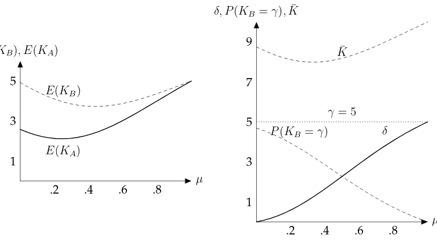
This does not mean however that a higher share of ex-ante indifferent consumers always increases expected investment at the margin. Figure 3 illustrates the influence of µon the different elements of equilibrium bidding strategies, for parameter values corresponding to Proposition 1. The aggregate effect is shown in the panel on the left-hand side of the Figure. We observe that the expected bid of the firm with the smallest initial endowmentB initially decreases withµ, and only comes back to its initial level when the share of ex-ante indifferent consumers goes to 1. The impact is much more positive for the firm with the highest initial endowmentA.
µ E(KB), E(KA)
.8 .6
.4 .2
1 3 5
E(KA)
E(KB)
µ δ, P(KB =γ),K¯
.8 .6
.4 .2
1 3 5 7 9
δ P(KB =γ)
¯
K
[image:18.595.95.529.109.350.2]γ = 5
Figure 3: Impact of the share of ex-ante indifferent consumersµ, withc= 0.1, γ = 5
andα = 3β. Left panel: equilibrium investment. Right panel: bidding strategies.
5.2
The impact of the threshold level on expected investment.
As in the previous subsection, it is instructive to consider two polar cases. For a thresh-old exactly equal to zero, all competition is for the entire population, and firms bid ag-gressively, in a setup identical to the classic all-pay auction. Forγ very high, we are in the case of Proposition 3; both firms bid in the way well known from the classic all-pay auction with the twist that the price equalsµonly. Since both firms have shares of loyal consumers, bidding is less aggressive and both firms obtain strictly positive expected profits.
For intermediate values of γ, we illustrate the effect of γ on expected investments in Figure 4. The vertical dotted lines represent the values of γ that delimit the zones corresponding to Propositions 1 to 3 of the paper. When the investment thresholdγ is small but strictly positive (part (i) of the graph, corresponding to Proposition 1) both firms compete for loyal users of their competitors. If firms were to compete for these loyal users with certainty, both would be willing to invest up toK = 1
both firms assign to investments above γ. As long asγ < 1−β
c , the highest investment below γ which is still included in the mixed strategy, δ, is lower than the maximum investment which would be chosen if the two firms agreed to compete only for new users. The probability mass on higher investment levels overcompensates this so that in total investments are higher when firms compete for the entire population. This ex-plains why bothE(KA)andE(KB)decrease withγ, and why the gap between the two increases, asAbecomes proportionally more often idle when the thresholdγincreases. In the intermediate part (ii) of Figure 4 corresponding to Proposition 2, the impact of γ on expected investments is ambiguous. For these intermediate values, the firm with the highest initial endowmentAstarts to invest much more aggressively. This is because for these values, and as opposed to Proposition 1, the probability mass P(KA) = 0 =
P(K = B) = γ decreases with the threshold γ, which implies that the firms become more and more symmetric in their bidding strategies, and less and less symmetric in their expected profits.
When γ reaches the level at which firms decide to only compete for ex-ante indif-ferent users, the expected investments in both types of equilibrium are the same and the expected level of investment is continuous inγ. As γ increases furhte,r the invest-ments remain constant because firms compete only for new users and therefore bidding behavior is independent of γ. This corresponds to the part (iii) of the Figure, and to Proposition 3.
6
Conclusion
pres-γ E(KA), E(KB)
12 11 10 9 8 7 6 5 4 3 2 1 1 2 3 4 5
E(KA)
E(KB)
γ = 1c1−α−β+α2
1−β
γ = 1−β
c
[image:20.595.132.480.111.350.2](ii) (iii) (i)
Figure 4: Expected equilibrium investment, withα = 0.4,β = 0.1andc= 0.1.
ence of loyal users in the market introduces an anticompetitive element that allows both firms to make positive profits in expectation.
References
AGHION, P., BLOOM, N., BLUNDELL, R., GRIFFITH, R. and HOWITT, P. (2005).
Compe-tition and innovation: an inverted-u relationship*.The Quarterly Journal of Economics,
120(2), 701–728.
ARBATSKAYA, M. (2007). Ordered search. The RAND Journal of Economics, 38 (1), 119–
126.
ARMSTRONG, M., VICKERS, J. and ZHOU, J. (2009). Prominence and consumer search. The RAND Journal of Economics,40(2), 209–233.
BAGWELL, K. (2007). The economic analysis of advertising.Handbook of Industrial
Orga-nization,3, 1701–1844.
BAYE, M. R., KOVENOCK, D. and DE VRIES, C. G. (1996). The all-pay auction with
BURDETT, K. and JUDD, K. L. (1983). Equilibrium price dispersion.Econometrica: Journal
of the Econometric Society, pp. 955–969.
FARRELL, J. and KATZ, M. L. (1998). The effects of antitrust and intellectual property
law on compatibility and innovation.Antitrust Bulletin,43, 609.
JIA, H. (2008). A stochastic derivation of the ratio form of contest success functions. Public Choice,135(3-4), 125–130.
KLEMPERER, P. (1987). Markets with consumer switching costs.The quarterly journal of
economics, pp. 375–394.
MOLDOVANU, B. and SELA, A. (2001). The optimal allocation of prizes in contests.
American Economic Review, pp. 542–558.
PASTINE, I. and PASTINE, T. (2002). Consumption externalities, coordination, and ad-vertising.International Economic Review,43(3), 919–943.
ROBERSON, B. (2006). The colonel blotto game.Economic Theory,29(1), 1–24.
Appendix
A
Proofs
A.1
Proof of Lemma 1
Proof. (i) Suppose firm A chooses any investmentK >0with certainty. Then, firm B can invest at any KB = K +ε and win with certainty so that firm A would be better off by choosing zero. Suppose firm A invests zero with probability 1. Then, firm B makes a profit arbitrarily close to max{1−α,1−γ} by either marginally overbidding A’s investment of zero or investing γ to win the entire population. But then firm A could ensure a positive profit by in turn marginally overbidding B’s investment so that this cannot be an equilibrium either. Thus, the equilibrium must be in mixed strategies.
(ii) Suppose firm A bids KA = K′
with strictly positive probability, PA(K′
) > 0. Hence, by marginally overbiddingKB =K′
+ǫ, firmB gets a strictly higher profit of at leastµPA(K′
)−cǫ. Hence, two firms never have an atom at the same level of investment because both would have a strict gain by marginally overbidding the other.
(iii) Suppose there is a gap in the support of firmi′
s strategy between some K′
and K′′
∈ (0, γ), whereFi(K′
) = Fi(K′′
)and K′
< K′′
. Firmj always strictly prefers to investK′
thanK′′
, as the expected benefit is the same and the expected cost is strictly lower. This implies that firmj also strictly prefersK′
, which violates the condition that a firms has the same expected profit over the support of her mixed strategy. The same reasoning applies to any K′
and K′′
> γ. It does not hold however ifK′
< γ andK′′
≥γ. This is why, if there is a gap in the support of the equilibrium strategy, it must be between aK′
< γ andK′′
≥ γ. DefineK−
i as the lower bound of the support of firm i’s investment strategy belowγ. IfKj =K−
strictly better off by bidding exactlyγ, as the expected probability of having the lower bid would be identical. The supports of both firms’ strategies are identical, because no firm wants to bid strictly above the upper bound of the other firm’s support, no firm can bid below zero, and no firm has an incentive to bid just below γ.
(iv) Suppose firm A bidsKA =K′
6
={0, γ}with strictly positive probability,PA(K′
)>
0. At equilibrium, this bid must also be in the support of firm B, unless it is exactly equal to γ. Else, firm A could bid a lower amount and keep the same expected gain for a lower cost. If the investment is in the support of firmB, firmB strictly prefers to bidKB = K′
+ǫ thanKB = K′
−ǫ, as the benefit discretely increases just above K′
. IfK′
= 0, this is possible, as firm B cannot bid a strictly negative amount. Else, this is only possible if the support of the equilibrium investment of firmB displays a gap belowK′
. By (iii), this is only possible atK′
=γ.
A.2
Proof of Proposition 1
Proof. For every investment of firm B belowγ which is contained in the support of the equilibrium strategy, the following condition has to hold:
(6) FB(K)µ+ lim
ε→0FB(γ −ε)α−cK = limε→0FB(γ−ε)α ⇒ FB(K) =
c µK
and for every investment equal to or aboveγ
(7) FB(K)−cK = lim
ε→0FB(γ−ε)α ⇒ FB(K) =cK + limε→0FB(γ −ε)α
If firm A chooses zero with positive probability, firm B’s mixed strategy must not contain an atom at zero. However, firm B must also be indifferent between all invest-ment levels in the support of its equilibrium mixed strategy. Denote B’s expected profit byE[ΠB]. Then, for allK < γ
FA(K)µ+ lim
ε→0FA(γ−ε)β−cK =E[ΠB]
⇒ FA(K) = c
µK +
E[ΠB]−limε→0FA(γ−ε)β
For every investment atγ or above having a lower investment than the competitor im-plies also losing their share of favorably biased users.
(9) FA(K)−cK =E[ΠB] ⇒ FA(K) =cK +E[ΠB]
From Lines (6) to (9) follows that firm A’s and firm B’s distribution functions have the same slopes. This is true in both the low and the high investment range. Since the slope is higher for investments below γ than for investments aboveγ, there exists δ∈(0, γ)such that for both firms
(10) FA(K) = FA(δ)andFB(K) = FB(δ)for allK ∈[δ, γ)
and thereforelimε→0FA(γ−ε) = FA(δ)andlimε→0FB(γ−ε) = FB(δ).
Neither firm has an incentive to strictly exceed the maximum investment of the other firm. This would increase cost but not increase the probability of winning. Thus, the maximum investment chosen by each firm must be identical in equilibrium, i.e., there exists a unique K such thatFA(K) = FB(K) = 1and for allε > 0, FA(K −ε) < 1and FB(K − ε) < 1. Since the distribution functions of firms A and B also have identical slopes forK ≥γ, the distribution functions of both firms are identical forK ≥γ:
(11) FA(K) = FB(K)for allK ≥γ
Combining Equations (7), (9), and (11) yieldsE[ΠB] =FB(δ)α. Starting with Line (8) and plugging in yields forK < γ
(12) FA(K) = c
µK+
FB(δ)α µ −
FA(δ)β µ
We solve (12) forFB(δ)and obtain
FB(δ) =FA(δ)µ+β
α − c αδ
We plug in from Line (6) and solve forFA(δ)to obtain
(13) FA(δ) = cδ
α µ(µ+β) +
1
µ+β
The flat part in the distribution functions (Equation (10)) implies together with the different shares of biased users that firm B chooses an investment equal toγ with a pos-itive probability while firm A’s strategy has an atom at zero. Since the two firms cannot have an atom at the same investment level, and since neither firm has an incentive to chooseδwith positive probability, the distribution function of firm A must be continu-ous in δ andγ. In addition, atγ the distribution functions of both firms take identical values. Thus, the following holds
(14) FA(δ) =FA(γ) =FB(γ)
SinceFB(K)is linear forK ≤δ, we can rewrite (7) as
(15) FB(γ) =cγ+ c
µδα
Taking Line (14) and plugging in from Line (13) on the left-hand side and from Line (15) on the right-hand side, we arrive at
cδ
α µ(µ+β) +
1
µ+β
=cγ+ c
µδα
⇔ δ=γ µ(µ+β)
µ+α−α(µ+β) =γ
(1−α)µ µ+α2
(16)
It is easily verified that
(1−α)µ < µ+α2 ⇒δ < γ
Finally, we derive the maximum investment levels. SupposeK > γ. Since the distri-bution functions stay constant at one for all investment levels above the maximum level chosen, we obtain the following condition
(17) cK +FB(δ)α= 1 ⇔cK = 1− c
µδ= 1−cγ
(1−α)µ µ(µ+α2)
whereδ has been derived in Equation (16). Rewriting (17) yields the maximum invest-ment level
K = 1
c −γ
As by assumption α+β+µ = 1, we replaceµ = 1−α−β in the above results to state Proposition 1.
For the derivation of the maximum investment, we have assumed K > γ. This is indeed true if
(18) 1
c −γ
1−α
µ+α2 > γ⇔γ <
1
c
µ+α2
1−β
Using the distribution functions, we observe that FA(δ) > FB(δ)so that firm B has a higher investment than firm A more often than the reverse. We compute expected investments as
E[KA] =
Z δ
0
c µxdx+
Z K
γ
cxdx
= c(1−α)2µγ2
2(µ+α2)2 +12c
(µ−α((1+α)cγ−α))2
c2(µ+α2)2 −γ2
E[KB] =
Z δ
0
c µxdx+
Z K
γ
cxdx+Prob(KB =γ)γ
= c(1−α)2µγ2
2(µ+α2)2 +12c
(µ−α((1+α)cγ−α))2
c2(µ+α2)2 −γ2
+c(α−β)γ2
µ+α2
It is easily verified thatE[KA]< E[KB]. By the properties of the mixed strategy equilib-rium, the expected profit of each firm equals its expected profit conditional on investing zero which is its endowment of loyal users multiplied with the probability of the com-petitor investing belowγ.
A.3
Proof of Proposition 2.
Proof. In the following, we deriveδ ∈(0, γ)such that both firms randomize over(0, δ), firm A chooses zero with positive probability and firm B choosesγwith positive proba-bility. In this equilibrium firm A chooses investments below or equal toδwith certainty, i.e.,FA(δ)whereas firm B also choosesγ such thatFB(δ)<1.
Since firm B could ensure profit 1−cγ by deviating to choosingγ, the distribution function of firm A must fulfill for allK ≤δ
(19) FA(K)µ+β−cK = 1−cγ⇒FA(K) = c
µK+
By assumption γ < 1−β
c and thus
1−β−cγ
µ > 0. Note that choosing γ also yields an expected profit equal to1−cγ for firm B.
Firm A obtains an expected profit equal to its share of loyal users multiplied by the probability that B chooses an investment invests less thanγ,FB(δ)α. For the distribution function of firm B and investmentsK ≤δthe following must hold:
FB(K)µ+α−cK =α⇔FB(K) = c
µK
The investment levelδis such that the distribution function of firm A just reaches 1 at this level
(20) c
µδ+
1−β−cγ
µ = 1 ⇔δ =γ − α
c
Ifγ < 1−β
c , thenδ < µ c.
Finally, we derive the probability with which firm B choosesγ.
Prob(KB =γ) = 1− c
µδ= 1−1 +
1−β µ −
c µγ =
1−β µ −
c µγ
From Line (19) also
Prob(KA = 0) = 1−β
µ − c
µγ =Prob(KB =γ)
Byγ < 1−β
c , it holds that Prob(KB =γ)>0. Moreover,
µ >0⇒µ+β > β ⇒(1−α)2 > β(1−α)⇒1−α−β+α2 > α−αβ ⇒ 1−α−β+α
2
1−β > α
and therefore
γ > 1 c
1−α−β+α2
1−β ⇒γ > α
c
so that Prob(KB=δ)<1. Byγ > 1c 1−β
1+α−β firm A does indeed not want to deviate to choosingγ:
γ > 1c 1−β
1+α−β ⇒cγ(µ+α)> µ+α
2 ⇔ −α2
µ + c
Using the distribution functions from Proposition 2, we observe thatFA(δ)> FB(δ), and we compute expected investments as
E[KA] =
Z δ
0
c
µxdx= c(α
c −γ)
2
2µ
E[KB] =
Z δ
0
c
µxdx+Prob(KB =γ)γ = c(α
c −γ)
2
2µ +γ
1−β−cγ µ
where obviouslyE[KA] < E[KB]. By the properties of the mixed strategy equilibrium, the expected profit of each firm equals its expected profit conditional on investing zero which is its endowment of loyal users multiplied with the probability of the competitor investing belowγ.
A.4
Proof of Corollary 1
Part (i)
Prob(nA=α+µ) =
Z δ
0
FB(K) c
1−α−βdx=
1 2c
2γ2 (1−α)2
(1−α−β+α2)2
Prob(nB =β+µ) =
Z δ
0
FA(K) c
1−α−βdx=
1 2c
2γ2(1−α)(1−β+ (α−β))
(1−α−β+α2)2
Prob(nA= 1) =
Z K
γ
FB(K)cdx= 1 2−
1 2c
2γ2 (1−β)2
(1−α−β+α2)2
Prob(nB = 1) =
Z K
γ
cFA(K)dx+Prob(KB =γ)FA(γ)
= 1 2−
1 2c
2γ2(1−β)(1−α−(α−β))
(1−α−β+α2)2
Prob(nA> α) =
Z δ
0
FB(K) c
(1−α−β)dx+
Z K
γ
FB(K)cdx
= 1 2−
1 2c
2γ2(α−β)(2−α−β)
(1−α−β+α2)2
Prob(nB > β) =
Z δ
0
FA(K) c
(1−α−β)dx+
Z K
γ
cFA(K)dx+Prob(KB =γ)FA(γ)
= 1 2+
1 2c
2γ2(α−β)(2−α−β)
(1−α−β+α2)2
whereδis defined in Line (16) asδ =γ(1−α)(1−α−β) 1−α−β+α2 .
Obviously, Prob(nB > β)>Prob(nA > α). Since1−α <1−α+(α−β)<1−β+(α−β)
it holds that Prob(nA =α+µ)<Prob(nB =β+µ). Moreover, since1−α−(α−β)<
Part (ii)
Prob(nA=α+µ) =
Z δ
0
FB(K) c
1−α−βdx=
(cγ−α)2
2(1−α−β)2
Prob(nB =β+µ) =
Z δ
0
FA(K) c
1−α−βdx=
(cγ−α)(2−cγ−α−2β) 2(1−α−β)2
Prob(nA= 1) = 0
Prob(nB = 1) =Prob(KB =γ) = (cγ−α)(2−cγ−α−2β) 2(1−α−β)2
Prob(nA> α) =Prob(nA=α+µ) = (cγ−α)
2
2(1−α−β)2
Prob(nB > β) = Prob(nB =β+µ) +Prob(nB = 1) = 1− (cγ−α)
2
2(1−α−β)2
whereδis defined in Line (20) asδ =γ− α c.
Part (iii) Since both firms invest only below γ, Prob(nA = 1) = Prob(nB = 1) = 0. Moreover, forK < γ the distribution functions of firms A and B are identical such that Prob(nA=α+µ) =Prob(nB =β+µ) = 1
2.
B
The user subgame
Perhaps the simplest way to derive utility functions consistent with our model is to as-sume loyal conas-sumers have an attention threshold atγ. All three types of users derive utility from the level of investment of the firm they choose. Consumers of typem are ex-ante indifferent, observe both firms and chose the one that provides the higher in-vestment. Consumers of types a and b belong to the exogenously given loyal base of firm A orB, respectively. They only observe the firm they are loyal to, unless the in-vestment of the other firm is above a threshold γ. For simplicity, we assume that the reservation utility of users is equal to0so that everyone joins a firm in equilibrium.
The utility of a consumer of typej ∈a, b, mwhen joining firmiis
Uj(i) =Ki (21)
the firm they are loyal correctly. But they pay attention to the alternative only if the competitor’s investment exceeds γ. Thus, a loyal consumers j ∈ {a, b} perceives her utility from joining the firmnshe is not loyal to to be
Uj(n) =
(
0iffKn < γ KniffKn ≥γ.
Each user joins the firm which maximizes her perceived utility. We assume that if indifferent between abstaining or joining a firm, users join. Hence, each consumer chooses the firm with the highest investment unless this consumer is loyal to a firm, the highest investment is lower thanγ, and it comes from a firm she is not loyal to.
The timing of the game is the following:
1. Firms A and B choose their investments simultaneously.
2. Users simultaneously decide which firm to join (‘user subgame’).
3. Payoffs realize.
The outcomes associated with pure-strategy equilibrium in the user subgame are of two types: If the entire population joins the same firm, this firm obtains a monopoly position with corresponding network sizesnA= 1,nB = 0ornA= 0,nB = 1. If instead loyal users remain with their firm and do not switch, we obtain competing networks where network sizes arenA=α,nB =β+µornA =α+µ,nB =β.
C
Probabilistic setting
In this section, we show that the fact that investment is deterministic with a discrete thresholdγ is not crucial to our results. Consider two firms, A and B choosing a level of investmentei, withi ∈ {A, B}, at costc(ei)with c′
> 0, c′′
> 0and c(0) = 0. Firms compete for users from a population of mass one. This population consists of three types of users,a, b, andm. Typesaandboccur with frequencyαandβ, respectively, in the population and the remaining part are of typem,µ= 1−α−β. The structure of the game and frequencies of types are common knowledge.
Suppose all types of customers intend to join the firm that maximizes their utility but may make mistakes and join the “wrong” firm. We employ the commonly used ratio-form contest success function which imposes that the probability of choosing one firm over the other equals its share in total investments.6
The ex-ante indifferent consumers choose firmiwith a probability
(22) pim(ei, ej) = ei
ei+ej.
The loyal consumers of typeichoose the firmithey are loyal to with a probability
(23) pii(ei, ej) = ei+γ
ei+ej+γ.
Therefore, the ex-ante loyal consumers of typej choose firmiwith a probability
(24) pij(ei, ej) = 1−p i
i(ei, ej) =
ei ei+ej +γ.
FirmAchooses the level of investment that maximizes her expected profit
(25) E(ΠA) =µpam(ea, eb) +αpaa(ea, eb) +βpab(ea, eb)−c(ea)
Solving the first-order condition of the profit maximization with respect toeayields
(26) c′
(ea) = βeb (ea+eb)2 +
eb(α+β) +βγ
(ea+eb+γ)2
Solving the same way for firmbyields
(27) c′
(eb) = µea (ea+eb)2 +
ea(α+β) +αγ
(ea+eb+γ)2
We immediately observe that:
(i) The equilibrium level of investment increases with the share of ex-ante indifferent consumers.
6Jia (2008) shows how such a contest success function can be derived from a model where the realized
(ii) The equilibrium level of investment decreases in the cost-efficiency (the c func-tion).
(iii) The firm that invests the most in equilibrium is the firm with the smallest share of loyal consumers.