Real Reward Testing for Probabilistic Processes
(Extended Abstract)Yuxin Deng1, Rob van Glabbeek2,4, Matthew Hennessy3&Carroll Morgan4
1 Shanghai Jiao Tong University, China 2
NICTA, Sydney, Australia 3 Trinity College Dublin, Ireland
4 University of New South Wales, Sydney, Australia
Abstract. We introduce a notion of real reward testing for probabilistic pro-cesses by extending the traditional nonnegative reward testing with negative re-wards. In this testing framework, the may and must preorders turn out to be the in-verse relations of each other. We show that for convergent processes with finitely many states and transitions, but not in the presence of divergence, the real re-ward must testing preorder coincides with the nonnegative rere-ward must testing preorder. To prove this coincidence we characterise the usual resolution based testing in terms of the weak transitions of processes, without involving policies, adversaries, schedulers, resolutions, or similar structures that are external to the process under investigation. This requires establishing the continuity of our func-tion for calculating testing outcomes.
1
Introduction
Extending the classical testing semantics [6,8] to a setting in which probability and nondeterminism co-exist was initiated in [14]. The application of a test to a process yields a set of probabilities for reaching a success state. Reward testing was introduced in [9]; here the success states are labelled by nonnegative real numbers—rewards—to indicate degrees of success, and reaching a success state amounts to accumulating the associated reward. In [13] an infinite set of success actions is used to report success, and the testing outcomes are vectors of probabilities of performing these success actions. Compared to [9] this amounts to distinguishing different qualities of success, rather than different quantities.
In [14] and [13], both tests and testees are nondeterministic probabilistic processes, whereas [9] allows nonprobabilistic tests only, thereby obtaining a less discriminating form of testing. In [5] we strengthened reward testing by also allowing probabilistic tests. Taking rewards testing in this form we showed that for finitary processes, i.e. finite-state and finitely branching processes, all three modes of testing lead to the same testing preorders. Thus, vector based testing is no more powerful than scalar testing that employs only one success action, and likewise reward testing is no more powerful than the special case of reward testing in which all rewards are 1.1
1
In certain occasions it is natural to introduce negative rewards. This is the case, for instance, in the theory of Markov decision processes [10]. Intuitively, we could under-stand negative rewards as costs, while positive rewards are often viewed as benefits or profits. This leads to the question: if negative rewards are also allowed, how would the
original reward testing semantics change? We refer to the more relaxed form of testing,
using positive and negative rewards, as real reward testing and the original one (from [9], but with probabilistic tests as in [5]) as nonnegative reward testing.
As remarked, [5] established that for finitary processes the nonnegative reward must testing preorder (⊑nrmust) coincides with the probabilistic must testing preorder (⊑pmust), and likewise for the may preorders. In the present paper, we show that, in
con-trast to the situation for nonnegative reward (or scalar) testing, for real reward testing the may and must preorders are the inverse of each other, i.e. for any processes∆and Λ,
∆⊑rrmay Λ iff Λ⊑rrmust∆. (1)
Our main result is that restricted to finitary convergent processes, the real reward must preorder coincides with the nonnegative reward must preorder, i.e. for any finitary con-vergent processes∆andΛ,
∆⊑rrmustΛ iff ∆⊑nrmustΛ. (2)
Here by convergence we mean that in the pLTS generated by a processes there is no infinite sequence of internal transitions between distributions like
∆0−→τ ∆1−→ · · ·τ
Although it is easy to see that in (2) the former implies the latter, to prove that the latter implies the former is far from trivial. Our proof strategy employs a novel characteri-sation of the usual resolution based testing approach, without using any concept like
policy [10], adversary [11], scheduler [12] or resolution [5] that is external to the
pro-cess under investigation; instead we describe the mechanism for gathering test results in terms of the weakτ-moves or derivations [2] the investigated process can make, and
hence speak of derivation based testing.
This allows us to exploit the failure simulation preorder⊑FSthat in [2] was proven to coincide with the probabilistic must testing preorder⊑pmustbased on resolutions, at
least for finitary processes. Using the derivational characterisation we can show that, for finitary convergent processes,⊑FSis contained in⊑rrmust. Convergence is essential here, even though it is not needed to establish that⊑FS is contained in⊑nrmust. Com-bining this with the results from [5] and [2] mentioned above leads to our required result that⊑nrmustis included in⊑rrmust, as far as finitary convergent processes are concerned. Consequently, all the relations in Figure 1 collapses into one.
(⊑rrmay)−1
Thm.2
= ⊑rrmust
Thm.5
= ⊑nrmust [5]
= ⊑pmust
[2]
= ⊑FS
The symbol=between two relations means that they coincide for finitary convergent processes.
Fig. 1. The relationship of different testing preorders.
In order to establish the agreement of resolution based testing with derivation based testing, we need to show that in the resolution based testing approach our results-collecting function in a deterministic labelled transition system is continuous, which involves some work on the continuity of real-valued functions.
The rest of this paper is organised as follows. We start by recalling notation for prob-abilistic labelled transition systems. In Section 3 we review the resolution based testing approach and show that the real reward may preorder is simply the inverse of the real reward must preorder. In Section 4 we present derivation based testing. The two results gathering mechanism are compared and shown to agree in Section 5. Then in Section 6 we show that for finitary convergent processes real reward must testing coincides with nonnegative reward must testing. We also present a counterexample showing that this result does not hold in the presence of divergence. We conclude in Section 7.
Due to lack of space, we omit all proofs: they are reported in [3]. Besides the re-lated work already mentioned above, a lot of other studies on probabilistic testing and simulation semantics have appeared in the literature. They are reviewed in [4,1].
2
Probabilistic Processes
A (discrete) probability subdistribution over a setS is a function∆ :S →[0,1]with P
s∈S∆(s) ≤ 1; the support of such a∆is⌈∆⌉:= {s∈S | ∆(s) > 0}, and its
mass|∆|isP
s∈⌈∆⌉∆(s). A subdistribution is a (total, or full) distribution if|∆|= 1.
The point distributionsassigns probability1tosand0to all other elements ofS, so that⌈s⌉ ={s}. WithDsub(S)we denote the set of subdistributions overS, and with
D(S)its subset of full distributions.
Let{∆k |k∈K}be a set of subdistributions, possibly infinite. ThenP
k∈K∆kis the real-valued function inS →Rdefined by(
P
k∈K∆k)(s) := P
k∈K∆k(s). This is a partial operation on subdistributions because for some statesthe sum of∆k(s)
might exceed1. If the index set is finite, say{1..n}, we often write∆1+. . .+∆n. Forp a real number from [0,1]we use p·∆ to denote the subdistribution given by
(p·∆)(s) := p·∆(s). Finally we useεto denote the everywhere-zero subdistribution that thus has empty support. These operations on subdistributions do not readily adapt themselves to distributions; yet ifP
k∈Kpk = 1for some collection ofpk ≥0, and the∆k are distributions, then so isP
k∈Kpk·∆k. In general when0≤p≤1we write xp⊕yforp·x+ (1−p)·ywhere that makes sense, so that for example∆1p⊕∆2is
always defined, and is full if∆1and∆2are. The expected valueP
s∈S∆(s)·f(s)over a subdistribution∆of a bounded non-negative functionf to the reals or tuples of them is written Exp∆(f), and the image of a subdistribution ∆ through a functionf is written Imgf(∆) — the latter is the subdistribution over the range off given by Imgf(∆)(t) :=P
Definition 1. A probabilistic labelled transition system (pLTS) is a triplehS, L,→i, where
(i) Sis a set of states,
(ii) Lis a set of transition labels,
(iii) relation→is a subset ofS×L× D(S).
A (non-probabilistic) labelled transition system (LTS) may be viewed as a degenerate pLTS — one in which only point distributions are used. As with LTSs, we writes−→α ∆ for(s, α, ∆)∈ →, as well ass−→α for∃∆:s−→α ∆ands→for∃α:s −→α . A pLTS is deterministic if for any statesand labelαthere is at most one distribution∆with s−→α ∆. It is finitely branching if the set{∆|s−→α ∆, α∈L}is finite for all states s; if moreoverSis finite, then the pLTS is finitary. A subdistribution∆in an arbitrary pLTS is finitary if restricting the state set to the states reachable from∆yields a finitary sub-pLTS; it is very finite if moreover it cannot reach any loop in the pLTS.
LetActbe a set of visible actions which processes can perform, and letτ 6∈Actbe the invisible or internal action. In this paper a (probabilistic) process will simply be a distribution in a pLTS with as set of transition labelsActτ :=Act∪ {τ}.
We graphically depict processes by drawing the part of the pLTS that is reachable from them as a directed graph with states represented by filled nodes•and distributions by open nodes◦. For any statesand distribution∆withs−→α ∆we draw an edge from sto∆labelled withα; and for any distribution∆and statesin⌈∆⌉, the support of∆, we draw an edge from∆toslabelled with∆(s). We leave out point-distributions— diverting an incoming edge to the unique state in its support.
3
Testing probabilistic processes
A test is a distribution in a pLTS with as set of transition labelsActτ ∪Ω, where Ω is a set of fresh success actions, not already inActτ, for reporting test outcomes. For simplicity we may assume a fixed pLTS of processes—our results apply to any choice of such a pLTS—and a fixed pLTS of tests. Since we need certain tests for testing processes, we have to postulate that the pLTS of tests has some degree of universality, in the sense that any test we may need is actually present in that pLTS. In previous papers [4,1,2] we accomplished this by presenting a language,pCSP, and taking an appropriate class ofpCSP expressions as the states of our pLTSs (of both tests and processes). Technically this works excellently, but it gives the impression that our work applies to one particular system description language only. Therefore we now achieve universality in a different way. Strong bisimulation between probabilistic processes is defined, for instance, in [7]. This notion can equally well be applied to relate states in different pLTSs. Now we achieve the desired degree of universality of our pLTS of tests by requiring that for any statesin any pLTS, such thatsis a very finite test, there is a state in our pLTS of tests that is strongly bisimilar to it.
t α
−→TΘ α6∈Act tkp α
−→Θkp
p α
−→P ∆ α6∈Act tkp α
−→tk∆
t a
−→TΘ p
a
−→P∆ a∈Act tkp τ
[image:5.612.145.473.114.144.2]−→Θk∆
Fig. 2. Synchronous parallel composition between tests and processes
(A) ift−→ω1 andt−→ω2 withω1, ω2∈Ωthenω1=ω2.
(B) ift−→ω withω∈Ωandt−→α ∆withα∈Actτthenu−→ω for allu∈ ⌈∆⌉. The first condition says that a success state can have one success identity only, whereas the second condition is slight weakening of the requirement from [9] that success states must be end states; it allows further progress from anω-success state, for someω∈Ω, but only when staying in the realm ofω-success states.2
To apply testΘ to process∆we form a parallel compositionΘk∆in which all visible actions of∆must synchronise withΘ. The synchronisations are immediately renamed intoτ. The resulting composition is a process whose only possible actions are the elements ofΩτ:=Ω∪{τ}. Formally, ifhP,Actτ,→PiandhT,Actτ∪Ω,→Tiare
the pLTSs of processes and tests, then the pLTS of applications of tests to processes is
hC, Ωτ,→i, withC={tkp|t∈T∧p∈P}and→the transition relation generated by the rules in Fig. 2. Here ifΘ∈ D(T)and∆∈ D(P), thenΘk∆is the distribution given by(Θk∆)(tkp) :=Θ(t)·∆(p).
Note that, since the pLTS of tests satisfies conditions (A) and (B) above, so does the pLTS of applications of tests to processes; this would not be the case if we had strengthened condition (B) to require that success states must be end states.
We will define the resultA(Θ, ∆)of applying the testΘto the process∆to be a set of testing outcomes, exactly one of which results from each resolution of the choices inΘk∆. Each testing outcome is anΩ-tuple of real numbers in the interval [0,1], i.e. a functiono:Ω→[0,1], and itsω-componento(ω), forω∈Ω, gives the probability that the resolution in question will reach anω-success state, one in which the success
actionωis possible.
Due to the presence of nondeterminism in pLTSs, we need a mechanism to reduce a nondeterministic structure into a set of deterministic structures, each of which deter-mines a possible outcome. Here we adapt the notion of resolution, defined in [5] for probabilistic automata, to pLTSs.
Definition 2 (Resolution). A resolution of a subdistribution∆∈ Dsub(S)in a pLTS
hS,Ωτ,→i is a triplehR, Γ,→Ri where hR,Ωτ,→Ri is a deterministic pLTS and Γ∈ Dsub(R), such that there exists a resolving functionf ∈R→Ssatisfying
(i) Imgf(Γ) =∆
(ii) ifr−→α RΓ′forα∈Ωτthenf(r)−→α Imgf(Γ′) (iii) iff(r)−→α forα∈Ω
τthenr−→α R.
The reader is referred to Section 2 of [5] for a detailed discussion of the concept of res-olution, and the manner in which a resolution represents a run of a process; in particular
τ
1/2 1/2
τ
ω τ
(c)
s s
s
s 2
3
4 1
a
ω τ
1/2 1/2
a
τ
q
1 t t||q1
[image:6.612.191.425.112.285.2](a) (b)
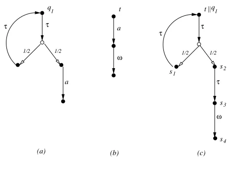
Fig. 3. Testing the processq1
in a resolution states in S are allowed to be resolved into distributions, and compu-tation steps can be probabilistically interpolated. Our resolutions match the results of applying a scheduler as defined in [12].
We now explain how to associate an outcome with a particular resolution, which in turn will associate a set of outcomes with a subdistribution in a pLTS. Given a determin-istic pLTShR,Ωτ,→iconsider the functionalR : (R →[0,1]Ω)→ (R → [0,1]Ω) defined by
R(f)(r)(ω) :=
1 ifr−→ω
0 ifr−→ω6 andr−→τ6
Exp∆(f)(ω) ifr−→ω6 andr−→τ ∆.
(3)
We view the unit interval[0,1]ordered in the standard manner as a complete lattice; this induces the structure of a complete lattice on the product[0,1]Ω and in turn on the set of functionsR→[0,1]Ω. The functionalRis easily seen to be monotonic and therefore has a least fixed point, which we denote byVhR,Ω
τ,→i; this is abbreviated to Vwhen the resolution in question is understood.
Now we defineA(Θ, ∆)to be the set of vectors
A(Θ, ∆) := {ExpΓ(VhR,Ω
τ,→i) | hR, Γ,→iis a resolution ofΘk∆}. (4)
Example 1. Consider the processq1depicted in Figure 3(a). When we apply the testt depicted in Figure 3(b) to it we get the processtkq1depicted in Figure 3(c). This process is already deterministic, hence has essentially only one resolution: itself. Moreover the outcome Exptkq
1(
V) =V(tkq1)associated with it is the least solution of the equation
V(tkq1) = 12·V(tkq1) +12−→ω
In fact this equation has a unique solution in[0,1]Ω, namely−→ω, with−→ω(ω) = 1and
−
1/2 1/2
τ
a
τ τ τ
1/2 1/2
τ
ω
(a)
τ τ
1/2 1/2
s1
s
3 4
a 1/2
ω τ
1/2
s2 s
a
ω
t q
2
(b) (c)
:= s0 t||q2
[image:7.612.137.480.95.297.2]s5 s6
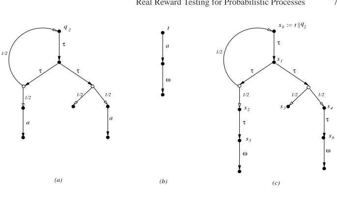
Fig. 4. Testing the processq2
Example 2. Consider the processq2and the application of the testtto it, as outlined in Figure 4. For eachk≥ 1the processtkq2 has a resolutionRk such thatV(Rk) =
(1− 1
2k)−→ω; intuitively it goes around the loop(k−1)times before at last taking the
right handτ action. ThusA(t, q2)contains(1− 1 2k)
−
→ω for everyk ≥ 1. But it also
contains−→ω, because of the resolution which takes the left handτ-move every time. ThusA(t, q2)includes the set
{(1−12)−→ω , (1−212)−→ω , . . . ,(1−
1
2k)−→ω , . . . ,−→ω}
As resolutions allow any interpolation between the two τ-transitions from states2,
A(t, q2)is actually the convex closure of the above set.
There are two standard methods for comparing two sets of outcomes:
O1≤HoO2 if for everyo1∈O1there exists someo2∈O2such thato1≤o2 O1≤SmO2 if for everyo2∈O2there exists someo1∈O1such thato1≤o2
This gives us our definition of the probabilistic may- and must-testing preorders; they are decorated with ·Ωfor the repertoireΩof testing actions they employ.
Definition 3 (Probabilistic testing preorders).
(i) ∆⊑Ω
pmayΛif for everyΩ-testΘ,A(Θ, ∆)≤HoA(Θ, Λ). (ii) ∆⊑Ω
pmustΛif for everyΩ-testΘ,A(Θ, ∆)≤SmA(Θ, Λ).
These preorders are abbreviated to∆⊑pmay Λand∆⊑pmustΛwhen|Ω|= 1.
In [5] we established that for finitary processes⊑Ω
pmay coincides with ⊑pmay and
⊑Ω
pmustwith⊑pmustfor any choice ofΩ. We also defined the reward testing preorders
by those states which can enable success actions. A reward tupleh ∈ [0,1]Ω is used to assign rewardh(ω)to success action ω, for eachω ∈ Ω. Due to the presence of nondeterminism, the application of a testΘto a process∆produces a set of expected rewards. Two sets of rewards can be compared by examining their supremum/infimum elements; this gives us two methods of testing called reward may/must testing. In [5] all rewards are required to be nonnegative, so we refer to that approach of testing as
nonnegative reward testing. If we also allow negative rewards, which intuitively can be
understood as costs, then we obtain an approach of testing called real reward testing. Technically, we simply let reward tupleshrange over the set[−1,1]Ω. Ifo∈ [0,1]Ω, we use the dot-producth·o = P
ω∈Ωh(ω)·o(ω). It can apply to a setO ⊆ [0,1]Ω so thath·O = {h·o|o∈O}. LetA ⊆ [−1,1]. We use the notation F
A for the supremum of setA, anddAfor the infimum.
Definition 4 (Reward testing preorders).
(i) ∆ ⊑Ω
nrmay Λ if for everyΩ-testΘ and nonnegative reward tuple h ∈ [0,1]Ω,
F
h· A(Θ, ∆)≤F
h· A(Θ, Λ). (ii) ∆ ⊑Ω
nrmust Λ if for every Ω-testΘ and nonnegative reward tuple h ∈ [0,1]Ω, d
h· A(Θ, ∆)≤dh· A(Θ, Λ). (iii) ∆ ⊑Ω
rrmay Λ if for every Ω-test Θ and real reward tuple h ∈ [−1,1]Ω,
F
h· A(Θ, ∆)≤F
h· A(Θ, Λ). (iv) ∆ ⊑Ω
rrmust Λ if for every Ω-test Θ and real reward tuple h ∈ [−1,1]Ω, d
h· A(Θ, ∆)≤dh· A(Θ, Λ).
This time we drop the superscriptΩifΩis countably infinite.
It is shown in Corollary 1 of [5] that nonnegative reward testing is equally powerful as probabilistic testing.
Theorem 1 ([5]). For any finitary processes∆andΛ,
(i) ∆⊑nrmayΛif and only if∆⊑pmayΛ.
(ii) ∆⊑nrmustΛif and only if∆⊑pmustΛ.
In this paper we focus on the real reward testing preorders⊑rrmayand⊑rrmust, by com-paring them with the nonnegative reward testing preorders⊑nrmayand⊑nrmust. We first show that, although the two nonnegative reward testing preorders are in general incom-parable, the two real reward testing preorders are simply the inverse relations of each other.
Theorem 2. For any processes ∆ andΛ, it holds that ∆ ⊑rrmay Λ if and only if
Λ⊑rrmust∆.
4
Derivation based testing
In this section we give an alternative definition of A(Θ, ∆). Our definition has four ingredients. First of all, for technical reasons we normalise our pLTS by removing all τ-transitions that leave a success state. This way an ω-success state will only have outgoing transitions labelledω.
Definition 5 (ω-respecting). A pLTShS, Ωτ,→iis said to beω-respecting whenever
s−→ω , for anyω∈Ω, impliess−→τ6 .
It is straightforward to modify the pLTS of applications of tests to processes into one that it isω-respecting, namely by removing all transitionss −→τ ∆ for statesswith s−→ω . With[Θk∆]we denote the distributionΘk∆in this pruned pLTS.
Secondly, we recall the definition of weak derivations from [2]. In a pLTS actions are only performed by states, in that actions are given by relations from states to distri-butions. But processes in general correspond to distributions over states, so in order to define what it means for a process to perform an action, we need to lift these relations so that they also apply to distributions. In fact we will find it convenient to lift them to subdistributions.
Definition 6. Let(S, L,→)be a pLTS andR ⊆S× Dsub(S)be a relation from states
to subdistributions. ThenR ⊆ Dsub(S)× Dsub(S)is the smallest relation that satisfies:
(i) sRΛimpliessRΛ, and
(ii) (Linearity)∆i R Λi fori∈Iimplies(P
i∈Ipi·∆i) R ( P
i∈Ipi·Λi)for any pi∈[0,1](i∈I) withPi∈Ipi≤1.
An application of this notion is when the relation is−→α forα∈Actτ; in that case we also write−→α for−→α . Thus, as source of a relation−→α we now also allow distributions, and even subdistributions. A subtlety of this approach is that for any actionα, we have ε −→α εsimply by takingI = ∅orP
i∈Ipi = 0in Definition 6. That turned out to makeεespecially useful for modelling the “chaotic” aspects of divergence in [2].
Definition 7 (Weak derivation). Suppose we have subdistributions∆, ∆→
k , ∆×k, for k≥0, with the following properties:
∆ = ∆→0 +∆×0 ∆→0 −→τ ∆→1 +∆×1
.. .
∆→k −→τ ∆→k+1+∆×k+1. ..
. Then we call∆′ := P∞
k=0∆
×
k a weak derivative of∆, and write∆ =⇒∆′to mean that∆can make a weak derivation to its derivative∆′.
There is always at least one derivative of any distribution (the distribution itself) and there can be many.
Definition 8 (Extreme derivatives). A state s in a pLTS is called stable if s −→τ6 ,
and a subdistributionΛis called stable if every state in its support is stable. We write ∆=⇒≻Λwhenever∆=⇒ΛandΛis stable, and callΛan extreme derivative of∆. Referring to Definition 7, we see this means that in the extreme derivation ofΛfrom ∆at every stage a state must move on if it can, so that every stopping component can contain only states which must stop: fors∈ ∆→k +∆×k we haves∈ ∆×k if and now
also only ifs−→τ6 . Moreover if the pLTS isω-respecting then whenevers∈∆→k , it is not successful, i.e.s−→ω6 for everyω∈Ω.
Lemma 1 (Existence of extreme derivatives).
(i) For every subdistribution∆there exists some (stable)∆′such that∆=⇒≻∆′. (ii) In a deterministic pLTS if∆=⇒≻∆′and∆=⇒≻∆′′then∆′=∆′′.
It is worth pointing out that the use of subdistributions, rather than distributions, is essential here. If ∆ diverges, that is if there is an infinite sequence of derivations ∆ −→τ ∆1 −→τ . . . ∆k −→τ . . ., then the only extreme derivative of∆ is the empty subdistributionε. For example, the only transition of a statetwith just a selfτ-loop is t−→τ t, and thereforetdiverges; consequently its unique extreme derivative isε.
The final ingredient in the definition of a set of outcomes of an application of a test to a process is the outcome of a particular extreme derivative. Note that all states s∈ ⌈Λ⌉in the support of an extreme derivative either satisfys−→ω for a uniqueω∈Ω, or haves6→.
Definition 9 (Outcomes). The outcome$Λ ∈[0,1]Ω of a stable subdistributionΛis given by$Λ(ω) =P
s∈⌈Λ⌉, s−→ω Λ(s).
Putting all four ingredients together, we arrive at a definition ofAd(Θ, ∆):
Definition 10. Let∆be apCSPprocess andΘanΩ-test. Then
Ad(
Θ, ∆) ={$Λ|[Θk∆] =⇒≻Λ}.
The role of pruning in the above definition can be seen via the following example.
Example 3. Letpbe a process that first does ana-action, to the point distributionq, and then diverges, by engaging in aτ-loopq −→τ q. Lettbe the test used in Examples 1 and 2. Thenpkthas a unique extreme derivationΘk∆ =⇒≻ ε, whereas[Θk∆]has a unique extreme derivation[Θk∆] =⇒≻ [qkω]. Here we give the nameω to the state reachable fromt with the outgoingω-transition. The outcome inAd(t, p)shows that
processppasses testtwith probability1, which is what we expect for state-based test-ing. Without pruning we would get an outcome saying thatppassestwith probability0. As this example is non-probabilistic, it also illustrates how pruning enables the standard notion of non-probabilistic testing to be captured by derivation testing.
Example 4. (Revisiting Example 1.) The pLTS in Figure 3(b) is deterministic and
un-affected by pruning; from part (ii) of Lemma 1 it follows thattkq1has a unique extreme derivativeΛ. MoreoverΛcan be calculated to be
X
k≥1
1 2k ·s3,
Example 5. (Revisiting Example 2.) The application of the test t to processes q2 is outlined in Figure 4(b). Consider any extreme derivative∆′froms0= [tkq2]; note that here again pruning actually has no effect. Using the notation of Definition 7, it is clear that∆×0 and∆→0 must beεands0respectively. Similarly,∆×1 and∆→1 must beεand s1respectively. Buts1is a nondeterministic state, having two possible transitions:
(i) s1−→τ Λ0whereΛ0has support{s0, s2}and assigns each of them the weight12 (ii) s1 −→τ Λ1 whereΛ1 has the support{s3, s4}, again dividing the mass equally
among them.
So there are many possibilities for∆2; it is easy to see from Definition 7 that in fact∆2 can be of the form
p·Λ0+ (1−p)·Λ1 (5)
for any choice ofp∈[0,1].
Let us consider one possibility, an extreme one wherepis chosen to be0; only the transition (ii) above is used. Here ∆→
2 is the subdistribution 12s4, and ∆→k = ε wheneverk > 2. A simple calculation shows that in this case the extreme derivative generated isΛe
1=12s3+ 1
2s6which implies that 1 2−→ω ∈ A
d(t, q2).
Another possibility for∆2isΛ0, corresponding to the choice ofp= 1in (5) above. Continuing with this derivation leads to∆3being 12·s1+1
2·p5; in other words∆
×
3 = 1
2 ·p5and∆
→
3 = 12 ·s1. Now in the generation of∆4from∆
→
3 once more we have to resolve a transition from the nondeterministic states1, by choosing some arbitrary p∈[0,1]in (5). Suppose that each time this arises we systematically choosep= 1, that is, we ignore completely the transition (ii) above. Then it is easy to see that the extreme derivative generated is
Λe0=X
k≥1
1 2k ·p5
which simplifies to the distributionp5. This in turn means that−→ω ∈ Ad(t, q2).
We have seen two possible derivations of extreme derivatives froms0. But there are many others. In general whenever∆→k is of the formq·s1we have to resolve the nondeterminism by choosing ap ∈ [0,1]in (5) above; moreover each such choice is independent. It turns out that every extreme derivative∆′ofs0is of the form
q·Λe0+ (1−q)Λe1
for some choice ofq∈[0,1], which implies thatAd(t, q2)is the convex closure of the
set{1 2
− →ω ,−→ω}.
5
Comparison of resolution and derivation based testing
The next proposition maintains that for each extreme derivative there is a corre-sponding resolution, and vice versa.
Proposition 1. Let∆be a subdistribution a pLTShS, Ωτ,→i.
(i) Suppose∆=⇒≻∆′. Then there is a resolutionhR, Γ,→
Riof∆, with resolving
functionf, such thatΓ =⇒≻RΓ′for someΓ′for which∆′ =Imgf(Γ′).
(ii) SupposehR, Γ,→Riis a resolution of a∆with resolving functionf.
ThenΓ =⇒≻RΓ′implies∆=⇒≻Imgf(Γ′).
Our next step is to relate the outcomes extracted from extreme derivatives to those extracted from the corresponding resolutions. This requires some analysis of the eval-uation functionV(−). We have to show that the functionRdefined in (3) and its least fixed pointV(−)are continuous, which is by no means trivial because it involves iden-tifying a class of binary functions that are conditionally continuous.
Definition 11 (Continuous functions). A chain in a complete latticeLis a sequence of elements{cn | n ≥0} satisfyingci ≤ ci+1. Obviously chains have least upper bounds which we denote byF
n≥0cn.A functionf :L→Lis said to be continuous if it preserves the least upper bounds of chains
f(G
n≥0
cn) = G
n≥0 f(cn)
The following technical lemma states that some binary functions satisfy the property of
bounded continuity, which allows the exchange of limit and sum operations. It plays a
crucial role in proving the continuity ofR.
Lemma 2 (Bounded continuity). Given a functionf:N×N→R≥0which satisfies the following three conditions:
C1. f is monotonic in its second argument, i.e.j1≤j2impliesf(i, j1)≤f(i, j2)for alli, j1, j2∈N.
C2. For anyi∈N, the limitlimj→∞f(i, j)exists. C3. Moreover, for anyn∈N, the partial sumSn=
Pn
i=0limj→∞f(i, j)is bounded, i.e. there exists somec∈R≥0such thatSn≤cfor alln≥0.
then it holds that
∞
X
i=0
lim
j→∞f(i, j) = limj→∞ ∞
X
i=0 f(i, j).
In other words, the function f is continuous conditioned by the fact that its partial sums are always bounded by a constant. By exploiting the above lemma, we obtain the following nice property.
Lemma 3. Consider a deterministic pLTShR,Ωτ,→i. The functionRdefined in (3)
is continuous.
defined by induction onn:
V0(r)(ω) = 0 for allω∈Ω
Vn+1=R(Vn)
ThenV=F
n≥0 Vn.This is used in the following central result.
Proposition 2. Let∆be a subdistribution in anω-respecting deterministic pLTS. If∆=⇒≻∆′thenV(∆) =V(∆′).
We are now ready to compare the two methods for calculating the set of outcomes associated with a subdistribution:
– using resolutions and the evaluation functionVfrom page 6;
– using extreme derivatives and the reward function$from Definition 9.
Corollary 1. In anω-respecting pLTShS, Ωτ,→i, the following statements hold.
(i) If∆=⇒≻∆′then there is a resolutionhR, Γ,→Riof∆such thatV(Γ) = $(∆′).
(ii) For any resolutionhR, Γ,→Riof∆, there exists an extreme derivative∆′ such
that∆=⇒≻∆′andV(Γ) = $(∆′).
Corollary 2. For any testΘand process∆we have thatAd(Θ, ∆) =A(Θ, ∆).
6
Agreement of nonnegative and real reward must testing
In this section we prove the agreement of⊑nrmust with⊑rrmustfor finitary convergent processes, by using failure simulation [2] as a stepping stone. We start with defining the weak action relations=α⇒forα∈Actτand the refusal relations−→A6 forA⊆Actthat are the key ingredients in the definition of the failure simulation preorder.
Definition 12. Let∆and its variants be subdistributions in a pLTShS,Actτ,→i. – Fora∈Actwrite∆=a⇒∆′ whenever∆=⇒∆pre −→a
∆post =⇒∆′. Extend this
toActτby allowing as a special case that=τ⇒is simply=⇒, i.e. including identity (rather than requiring at least one−→τ ).
– ForA⊆Actands∈Swrites−→A6 ifs−→α6 for everyα∈A∪ {τ}; write∆−→A6 if s−→A6 for everys∈⌈∆⌉.
– More generally write∆=⇒ 6−→A if∆=⇒∆prefor some∆presuch that∆pre −→A6 .
Definition 13 (Failure simulation preorder). DefineFS to be the largest relation in
S× Dsub(S)such that ifsFSΛthen
(i) whenevers=α⇒∆′, forα∈Act
τ, then there is aΛ′∈ Dsub(S)withΛ=α⇒Λ′and
∆′ FSΛ
′, and
(ii) whenevers=⇒ 6−→A thenΛ=⇒ 6−→A .
Any relationR ⊆ S× Dsub(S)that satisfies the two clauses above is called a failure
simulation. The failure simulation preorder⊑FS ⊆ Dsub(S)× Dsub(S)is defined by
There are other equivalent definitions of failure simulation preorder [2]. This one is chosen because we find it convenient to use in proving Lemma 4 below.
The failure simulation preorder is a preserved under parallel composition with a test, followed by pruning, and it is sound and complete for probabilistic must testing preorder, when only finitary processes are considered.
Theorem 3 ([2]). For finitary processes∆andΛ,
(i) If∆⊑FS Λthen for anyΩ-testΘit holds that[∆kΘ]⊑FS [ΛkΘ].
(ii) ∆⊑FS Λif and only if∆⊑pmustΛ.
Because we prune our pLTSs before extracting values from them, we will be con-cerned mainly withω-respecting structures. Moreover, we require the pLTSs to be
con-vergent in the sense that there is no wholly dicon-vergent states, i.e. withs=⇒ε.
Definition 14. Let∆be a distribution in a pLTShS, Ωτ,→i. We writeV(∆)for the set of testing outcomes{$∆′|∆=⇒≻∆′}.
Lemma 4. Let∆andΛbe two subdistributions in anω-respecting convergent pLTS hS, Ωτ,→i. IfΛ⊑FS ∆, then it holds thatV(Λ)⊇ V(∆).
This lemma shows that failure simulation preorder is a very strong relation in the sense that ifΛ is related to ∆by the failure simulation preorder then the set of outcomes generated byΛincludes the set of outcomes given by∆. It is mainly due to this strong requirement that we can show that the failure simulation preorder is sound for the real reward must testing preorder. Convergence is a crucial condition in this lemma. Theorem 4. For any finitary convergent processes∆andΛ, if∆⊑FS Λthen we have
that∆⊑rrmustΛ.
The proof of the above theorem is subtle. The failure simulation preorder is defined via weak derivations (cf. Definition 13), while the reward must testing preorder is defined in terms of resolutions (cf. Definition 4). Fortunately, we have shown in Corollary 2 that we can just as well characterise the reward must testing preorder in terms of derivations. Based on this observation, the proof can be carried out by exploiting Theorem 3(i) and Lemma 4.
Finally, by combining Theorems 1(ii) and 3(ii), together with Theorem 4, we obtain the main result of the paper which states that nonnegative reward must testing is as discriminating as real reward must testing.
Theorem 5. For any finitary convergent processes∆andΛ, it holds that∆⊑Ω
rrmustΛ if and only if∆⊑nrmustΛ.
In the presence of divergence,⊑rrmustis strictly finer than⊑nrmust. For example, let
∆be a process that diverges, by performing aτ-loop only, andΛa process that merely performs a single actiona. It holds that∆ ⊑FS Λ because∆ =⇒ εand the empty subdistribution can failure simulate any processes. It follows from Theorems 3(ii) and 1(ii) that∆⊑nrmust Λ. However, if we apply the testtfrom Example 1 again, and the reward tuplehwithh(ω) =−1, then
F
h· Ad(t, ∆) = F
h· {ε} = F
{0} = 0
F
h· Ad(t, Λ) = F
h· {−→ω} = F
{−1} = −1
AsF
h· Ad(t, ∆)6≤F
7
Conclusion
We have studied a notion of real reward testing which extends the traditional nonneg-ative reward testing with negnonneg-ative rewards. It turned out that real reward may preorder is the inverse of real reward must preorder, and vice versa. More interestingly, for fini-tary convergent processes, real reward must testing preorder coincides with nonnegative reward testing preorder. In order to prove this result, we have presented two testing ap-proaches and shown their coincidence, which involved proving some analytic properties such as the continuity of a function for calculating testing outcomes, and bounded con-tinuity of a class of binary functions.
Although for finitary convergent processes, real reward must testing is no more powerful then nonnegative reward must testing, a similar result does not hold for may testing. This follows immediately from our result that (the inverse of) real reward may testing is as powerful as real reward must testing, that is known not to hold for non-negative reward may and must testing. Thus, real reward may testing is strictly more discriminating than nonnegative reward may testing, even in the absence of divergence.
References
1. Y. Deng, R.J. van Glabbeek, M. Hennessy & C.C. Morgan (2008): Characterising testing
preorders for finite probabilistic processes.Logical Methods in Computer Science 4(4:4). 2. Y. Deng, R.J. van Glabbeek, M. Hennessy & C.C. Morgan (2009): Testing finitary
proba-bilistic processes. In Proc.CONCUR’09, LNCS 5710, Springer, pp. 274–288.
3. Y. Deng, R.J. van Glabbeek, M. Hennessy & C.C. Morgan (2010): Real Reward Testing for
Probabilistic Processes. Full version of the current paper. Available athttp://basics. sjtu.edu.cn/˜yuxin/temp/reward.pdf.
4. Y. Deng, R.J. van Glabbeek, M. Hennessy, C.C. Morgan & C. Zhang (2007): Remarks on
testing probabilistic processes.ENTCS 172, pp. 359–397.
5. Y. Deng, R.J. van Glabbeek, C.C. Morgan & C. Zhang (2007): Scalar outcomes suffice for
finitary probabilistic testing. In Proc.ESOP’07, LNCS 4421, Springer, pp. 363–378. 6. R. De Nicola & M. Hennessy (1984): Testing equivalences for processes.Theoretical
Com-puter Science 34, pp. 83–133.
7. H. Hansson & B. Jonsson (1990): A calculus for communicating systems with time and
probabilities. In Proc.RTSS’90, IEEE Computer Society Press, pp. 278–287. 8. M. Hennessy (1988): An Algebraic Theory of Processes. MIT Press.
9. B. Jonsson, C. Ho-Stuart & Wang Yi (1994): Testing and refinement for nondeterministic
and probabilistic processes. In Proc.FTRTFT’94, LNCS 863, Springer, pp. 418–430. 10. M. Puterman (1994): Markov Decision Processes. Wiley.
11. J. Rutten, M. Kwiatkowska, G. Norman & D. Parker (2004): Mathematical Techniques for
Analyzing Concurrent and Probabilistic Systems, P. Panangaden and F. van Breugel (eds.),
CRM Monograph Series 23. American Mathematical Society.
12. R. Segala (1995): Modeling and Verification of Randomized Distributed Real-Time Systems. PhD thesis, MIT.
13. R. Segala (1996): Testing probabilistic automata. In Proc.CONCUR’96, LNCS 1119, Springer, pp. 299–314.