Learning based superresolution land cover mapping

Learning based super-resolution land cover mapping

Feng Ling, Yihang Zhang, Giles M. Foody IEEE Fellow, Xiaodong Li,

Xiuhua Zhang, Shiming Fang, Wenbo Li, Yun Du

This work was supported in part by the National Basic Research Program (973 Program) of China under Grant

No. 2013cb733205, and in part by Natural Science Foundation of Hubei Province for Distinguished Young

Scholars under Grant No. 2013CFA031.

F. Ling, Y. Zhang, X. Li, and Y. Du are with the Key Laboratory of Monitoring and Estimate for Environment

and Disaster of Hubei Province, Institute of Geodesy and Geophysics, Chinese Academy of Sciences, Wuhan

430077, China (e-mail: [email protected]).

G. M. Foody is with the School of Geography, University of Nottingham, University Park, Nottingham NG7

2RD, UK

X. Zhang is with the Wuhan Institute of Technology, Wuhan 430205, China

S. Fang is with the School of Public Administration, China University of Geosciences, Wuhan 430074, China.

W. Li is with the Hefei Institute of Technology Innovation, Chinese Academy of Sciences, Hefei, 230088, China.

*

Abstract: Super-resolution mapping (SRM) is a technique for generating a fine spatial resolution land cover

map from coarse spatial resolution fraction images estimated by soft classification. The prior model used to

describe the fine spatial resolution land cover pattern is a key issue in SRM. Here, a novel learning based SRM

algorithm, whose prior model is learned from other available fine spatial resolution land cover maps, is proposed.

The approach is based on the assumption that the spatial arrangement of the land cover components for mixed

pixel patches with similar fractions is often similar. The proposed SRM algorithm produces a learning database

that includes a large number of patch pairs for which there is a fine and coarse spatial resolution representation

for the same area. From the learning database, patch pairs that have similar coarse spatial resolution patches as

those in input fraction images are selected. Fine spatial resolution patches in these selected patch pairs are then

used to estimate the latent fine spatial resolution land cover map, by solving an optimization problem. The

approach is illustrated by comparison against state-of-the-art SRM methods using land cover map subsets

generated from the USA’s National Land Cover Database. Results show that the proposed SRM algorithm better

maintains the spatial pattern of land covers for a range of different landscapes. The proposed SRM algorithm has

the highest overall accuracy and Kappa values in all these SRM algorithms, by using the entire maps in the

accuracy assessment.

I. Introduction

Super-resolution mapping (SRM), which is also referred to sub-pixel mapping, is a method to generate fine

spatial resolution land cover maps from coarse spatial resolution remote sensing images. SRM can be viewed as

the post-processing of soft classification to further address the mixed pixel problem that is common in coarse

spatial resolution images [1, 2]. In general, soft classification estimates the fraction images that illustrate the area

percentage cover of land cover classes within coarse spatial resolution mixed pixels. The fraction images may be

input to a SRM analysis to predict the spatial locations of the land cover class at a fine spatial resolution. The

output of the SRM analysis is a hard classification land cover map, which has a finer spatial resolution than that

of input fraction images. At present, SRM has become a promising method to reduce the mixed pixel problem

that is widely encountered with coarse spatial resolution images, and has been successfully used in many

applications, such as mapping waterlines [3-5], lakes [6], urban buildings [7], urban trees [8], forests [9], as well

as in ground control point refinement [10] and the calculation of landscape pattern indices [11].

A large number of SRM algorithms have been proposed [12-27]. Generally, SRM is an ill-posed problem

[28], and the prior information about the spatial pattern of different land cover classes at the fine spatial

resolution scale needs be known before SRM is performed. Therefore, in order to estimate the latent fine spatial

resolution land cover map from input coarse spatial resolution fraction images, one of the key issues is the

definition of the prior model. The latter has been described from different perspectives. In the simplest case,

when only the coarse spatial resolution fraction images are available, the prior model is often based on the spatial

dependence principle, which aims to make the fine spatial resolution land cover map have the maximal spatial

dependence [1]. In practice, the spatial dependence of a certain fine spatial resolution pixel can be calculated by

comparing it with its neighboring fine spatial resolution pixels [14], fractions of its neighboring coarse spatial

proposed to describe the spatial land cover pattern more precisely [31], especially for some special land cover

classes [7, 32]. The spatial dependence model is a popular model for use in SRM due to its simplicity and

absence of requirements for additional information about the spatial pattern of the land cover. However, the

model can be inappropriate for areas with complex land cover patterns. The use of the wrong prior model in a

SRM analysis can result in an inappropriate and inaccurate land cover representation, possibly even worse than

that of a standard hard classification of the coarse resolution image in some cases [6, 33].

A promising approach to improve the effectiveness of the prior model is through the incorporation of

additional information on the land cover to inform the SRM analysis. Various approaches have been used. An

intuitive additional dataset to use in a SRM analysis is another kind of fine spatial resolution images, such as a

panchromatic band image [34-37] or a fine spatial resolution synthetic aperture radar (SAR) image [38]. Fine

spatial resolution digital elevation model [4, 5] and light detection and ranging (LIDAR) data [39], and vector

datasets [40] have also been successfully used to refine SRM analyses. Multiple sub-pixel shifted coarse spatial

resolution images which are used as an alternation datasets to provide additional information about the spatial

land cover pattern [41] for SRM, and this method has been further developed [6, 42-45]. A historical fine spatial

resolution land cover map can also be used to help the SRM analysis [9, 46, 47]. Adding site-specific additional

datasets can increase the accuracy of SRM, however, this kind of approach is often limited because the

additional dataset should cover the same area, in its entirety, as the input fraction images, and this may often not

be the case with the additional data only available for part of the region being mapped.

In addition to the aforementioned approaches, the spatial land cover pattern can also be learned from the

training image, which is often a fine spatial resolution land cover map that has a similar spatial land cover

pattern to the objective fine spatial resolution land cover map. In this situation, SRM predicts the fine spatial

that is learned from these training fine spatial resolution land cover maps. One kind of learning based SRM

algorithm uses a model to describe the fine spatial resolution land cover pattern, and the parameters of the prior

model are learned from the training maps [48-50]. Central to this kind of approach is the selection of the prior

model. Presently, a popular approach is to use a semi-variogram based approach in which the SRM aims to

produce a fine spatial resolution land cover map that has the same spatial pattern as that represented by the

semi-variogram fitted to the available fine spatial resolution land cover map. A critical drawback of this category

of SRM algorithms is, however, that the geo-statistical methodologies are constructed based on the assumption

of spatial stationary, and they are limited for complex land cover patterns which are often non-stationary.

Another kind of learning based SRM algorithms directly learns the relationship between coarse spatial

resolution fraction images and the fine spatial resolution land cover maps without a predefined model [51-54].

The basic assumption of this method is that the fine spatial resolution spatial land cover pattern is similar for a

mixed pixel patch, which is basically a block of coarse resolution pixels, with similar land cover class fractional

composition. Several algorithms have been proposed to learn the relationship, including the back-propagation

(BP) neural networks [51-54], and the support vector regression algorithms [55]. The SRM algorithms belonging

to this category often include two steps. In the first step, a fine spatial resolution image is estimated for each land

cover class using the learned relationship. In the second step, fine spatial resolution pixel labels are assigned with

the maximum a posteriori principle using all of these estimated fine spatial resolution images and input fraction

images as constraints. This kind of learning based SRM algorithm are special cases of the interpolation-based

SRM algorithm [56]; only the interpolation step is performed by the learning based methods. As a result, the

limitation of the interpolation-based SRM algorithm, notably salt-and-pepper and linear artifacts, is unavoidable

for this category of learning based SRM algorithm.

resolution mixed pixel patches with similar fractions have a similar fine spatial resolution land cover pattern.

Different to other learning based SRM algorithms, the novelty of the proposed learning based SRM algorithm

lies in the way the coarse spatial resolution and fine spatial resolution patches are used within the analysis. The

proposed method does not need the additional label assignment step and patch outliers are effectively addressed

during the analysis, avoiding commonly encountered error sources in other two-step learning based SRM

algorithms. The remainder of this paper is organized as follows. Section II details the proposed learning based

SRM algorithm. Section III validates the performance of the proposed algorithm through several experiments.

Section IV discusses some issues about the proposed algorithm and Section V concludes this paper.

II. Methods

A. Problem description

Suppose that the original coarse spatial resolution remotely sensed image has MN pixels and the

number of land cover classes in the whole image is C. It is assumed that the fraction images F for all classes

have been estimated by soft classification. The SRM analysis aims to generate a fine spatial resolution land

cover map H using F as input. By setting the zoom factor to be z, each coarse spatial resolution pixel is

divided into z z fine spatial resolution pixels. All fine spatial resolution pixels are considered to be pure

pixels and each one should be assigned to a single land cover class. The resulting fine spatial resolution land

cover map thus contains (z M ) ( z N) pixels, whose labels are defined to a unique class of C.

In this paper, it is assumed that fraction images F are exactly estimated without error. In each coarse

spatial resolution pixel V , the number of fine spatial resolution pixels Q Vc( ) assigned to the class

(1, 2, , )

c L C is computed according to the equation:

2 ,

( ) round( ( ) )

c F c

Q V  f V z (1)

resolution pixel V in the fraction images F, round( )x returns the value of the closest integer to x. In this

situation, the objective of the SRM analysis is to arrange these fine spatial resolution pixels within each coarse

spatial resolution pixel to make the fine spatial resolution land cover map honor a pre-defined spatial pattern

model.

For the proposed learning-based SRM algorithm, it is assumed that there are a set of fine spatial resolution

land cover maps available. These fine spatial resolution maps could be historical land cover maps or land cover

maps derived from fine spatial resolution remote sensing images. These available fine spatial resolution land

cover maps are used to provide information about the spatial land cover patterns at the fine spatial resolution.

Then, assuming that a mixed pixel patch with similar fractions has similar spatial land cover pattern, the SRM

analysis may yield a fine spatial resolution map.

B. The fine and coarse spatial resolution patch pair

For the land cover class c, the spatial land cover pattern is represented by the patch pair [ ,x yc c], in which

c

y is a coarse spatial resolution patch and its corresponding fine spatial resolution patch is x_c. Here, square

patches of size p are used with a coarse spatial resolution patch including pp coarse spatial resolution

pixels. The coarse spatial resolution patch is represented by the vector yc [fc(1),fc(2),L,fc(pp)], where

( ) c

f V is the fraction value of the coarse spatial resolution pixel V of the class c. The corresponding fine

spatial resolution patch includes z  p z p fine spatial resolution pixels, and is represented by the vector

[ (1), (2), , ( )]

c c c c

x  I I L I z  p z p , where I vc( ) is an indicator number showing whether a fine spatial

resolution pixel v belongs to the class c, and is defined as:

1 if fine spatial resolution pixel labelled with the land cover class ( )

0 otherwise

c

v c

I v  

 (2)

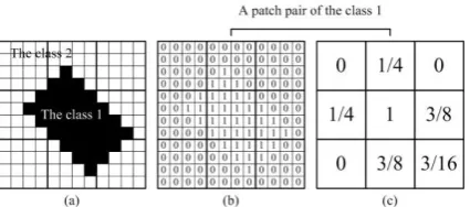
Fig. 1. A patch pair example, where the zoom factor is 4 and the coarse spatial resolution patch size is 3. (a) is a fine spatial

resolution land cover map including 12×12 pixels of two land cover classes, 1 (black) and 2 (white); (b) is the corresponding fine

resolution patch of the class 1, where the number 1 indicates that the fine resolution pixel belongs to the class 1, and 0 indicates that

the fine resolution pixel belongs to other classes; (c) is the corresponding coarse resolution patch, where the number within pixels is

the area percentages of the class 1 in each coarse spatial resolution pixel.

Fig. 1 shows a patch pair example with p3 and z4. Fig. 1(a) is a fine spatial resolution land cover

map including two classes. For the land cover class 1, as shown in black in Fig. 1(a), the fine and coarse spatial

resolution land cover patches are shown in Fig. 1(b) and Fig. 1(c), respectively. The fine spatial resolution patch

is an indicator map [Fig. 1(b)], where a label 1 means that the fine pixel belongs to the class 1, and 0 means that

the fine spatial resolution pixel belongs to other classes. Therefore, the indicator map

1

The first line The 5th line The 12th line

[0, 0,..., 0,..., 0, 0, 0,1,1,1,1,1, 0, 0, 0, 0,..., 0, 0,..., 0]

x  _{14442 4443 14444444442 4444444443 14442 4443 shows the spatial pattern of the class 1. The coarse patch is}

the fraction image of the class, where the value represents the area percentages within each coarse pixel, and is

represented as ₁ [0, , 0, ,1, , 0, ,1 1 3 3 3] 4 4 8 8 16

y  . Together [ ,x y_{1 1}] is a patch pair for the class 1.

Once a large number of patch pairs available, the SRM problem can then be solved by using a pattern

matching method. Given a coarse spatial resolution patch in the input fraction images, the patch pairs that have

similar coarse spatial resolution patches are selected from those available patch pairs. These selected patch pairs

are called as neighboring patch pairs, because if all patch pairs are listed in order according to the fraction values,

they are located in neighboring sites. It is noted that these neighboring patch pairs all include a coarse spatial

fraction values often have similar spatial land cover patterns, the latent fine spatial resolution patch for the coarse

spatial resolution patch in the input fraction images should be similar with the fine spatial resolution patch

included in the neighboring patch pairs. Thus, the SRM seeks to make the spatial land cover pattern of the

resultant fine spatial resolution land cover map match those of neighboring patch pairs.

In general, in the proposed learning based SRM algorithm, the fine and coarse spatial resolution patch pairs

are first extracted from available fine spatial resolution land cover maps to produce a learning database. Similar

patch pairs are then found for each coarse spatial resolution patch in input fraction images. Finally, these

available patch pairs in the learning database are used to reconstruct the final fine spatial resolution land cover

map. All these steps are described in detail as follows.

C. Generating the training database

Finding the relationship between the fine spatial resolution land cover maps and coarse spatial resolution

fraction images, which is represented by patch pairs in the training database, is one of the key issues of the

proposed learning based SRM algorithm. Here, the patch pairs are generated class by class. Given a set of fine

spatial resolution land cover maps, a corresponding set of coarse spatial resolution patches for each land cover

class can be produced from them.

An example fine spatial resolution land cover map which includes three land cover classes, as shown in Fig.

2(a), is used to illustrate the training database generation procedure. Before the training database is generated,

the zoom factor z and the coarse spatial resolution patch size p are set. In this example, z is set to be 4,

and p is set to be 3. A fine spatial resolution patch then includes z  p z p fine spatial resolution pixels

(equals to 12×12 in this example). In order to generate a patch pair, a fine spatial resolution land cover map

with the size of z  p z p is first exacted. Generally, by moving a fixed window containing z  p z p

These extracted fine spatial resolution maps can be overlapped, thus the fine spatial resolution land cover pattern

included in the original land cover map is fully exploited. For an extracted fine spatial resolution map, as shown

in Fig. 2(b), one fine spatial resolution patch, that is, one indicator map was then generated for each land cover

class, as shown in Fig. 2(c)-(e). For each fine spatial resolution patch, the corresponding coarse spatial resolution

patch consists of fraction values of all coarse spatial resolution pixels. Each coarse spatial resolution pixel

corresponds to z z fine spatial resolution pixels, and the fraction value f_c( )V , which is the percentage of the

fine spatial resolution pixels assigned to the class c in the coarse spatial resolution pixel V , is calculated as:

2

( ) ( )

c c

v V

f V I v z







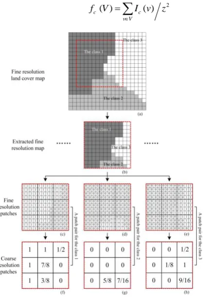
Fig. 2. An example of the training database generation procedure, where the zoom factor is 4 and the coarse resolution patch size is

3. (a) is the original fine resolution land cover map; (b) is one fine resolution land cover map including 12 12 fine resolution

pixels extracted from the original fine resolution land cover map. (c), (d) and (e) are fine resolution patches of different land cover

classes, which are generated from the extracted fine resolution land cover map. The number 1 indicates that the fine resolution pixel

belongs to the class, and 0 indicates that the fine resolution pixel belongs to other classes; (f), (g) and (h) are corresponding coarse

resolution patches generated from (c), (d) and (e), where the number within pixels means the area percentages of different class in

each coarse resolution pixel. One fine resolution patch and one coarse resolution patch form a patch pair, including (c) and (f), (d)

Each extracted fine spatial resolution map (Fig. 2) can generate one patch pair for each land cover class.

Supposed that K different fine spatial resolution maps are extracted from the original fine spatial resolution

land cover map, K patch pairs can be generated for each class. Those patch pairs comprise the training

database, where the fine spatial resolution patches are represented as _, { i_, }K₁ T c T c i

X  x _ and the coarse spatial

resolution patches are represented as , { , } 1

i K T c T c i

Y  y _ for class c.

D. Searching neighboring patch pairs

Once the training database has been built, it is used to provide land cover information to estimate the latent

fine spatial resolution land cover map with input coarse spatial resolution fraction images. For each coarse

spatial resolution patch in the input fraction images, neighboring training patch pairs that have similar coarse

spatial resolution patch are searched from the training database. Since the training database is generated class by

class, the search procedure is also performed class by class. Let _, { i_, }R₁ F c F c i

Y  y _ be coarse spatial resolution

patches in the input fraction images F for class c. For the ithcoarse spatial resolution patch ,

i F c

y , its

neighboring training patch pairs are chosen according to the following criterion:

, , 2

, , , ,

1

( i , i j) ( i ( ) i j( ))

F c T c F c T c L

f y y f V f V T

p p

   





where ,

, ,

( i , i j) F c T c

f y y

 is the difference of fraction values between coarse spatial resolution patch i_, F c

y in the

fraction image and the

j

th

i j T c

y in the training database. i_, ( ) F c

f V is the fraction value of

the class c of the coarse spatial resolution pixel V in i_, F c

y , and , , ( )

i j T c

f V is the fraction value of the class c

of the corresponding coarse spatial resolution pixel V in , ,

i j T c

y . The more similar the coarse spatial resolution

patches are, the lower the value of f . The threshold TL is the tolerable fraction difference between two

patches. If the value of , , ,

( iF c, T ci j)

f y y

 is no more than that of T_L,

y

,

i F c

important parameter for searching neighboring patch pairs. If it is too large, the neighboring patch pairs are too

different with that of the input fraction images to provide accurate land cover information. On contrast, if T_L is

too small, only few neighboring patch pairs can be found, leading to insufficient land cover information. The

effect of the value of T_L will be assessed in our later experiments.

The k-dimensional (K-D) tree algorithm is applied to find neighboring training patch pairs in the present

work, due to its efficient and successful application in the image super-resolution field [57]. The K-D tree

organizes coarse spatial resolution patches in the training database off-line to enable a fast search by defining a

binary tree of thresholds, which are chosen optimally so as to expedite the search. Moreover, the K-D tree relies

on a special high dimensional data structure and thus the neighbors searching step can be speeded up

significantly. More detailed information about the K-D tree can be found in references [57, 58].

For each coarse spatial resolution patch in the input fraction images F, the neighboring coarse spatial

resolution patches and their corresponding fine spatial resolution patches are searched from the training database

using the K-D tree algorithm. A simple example for a two class situation given in Fig. 3 is used to illustrate the

neighboring training patch pairs searching procedure. In this example, the coarse spatial resolution patch size p

is set to be 3, and one coarse spatial resolution patch then includes 3 × 3 coarse spatial resolution pixels. For a

coarse spatial resolution pixel in the fraction image, all nine coarse spatial resolution patches that include this

coarse spatial resolution pixel are extracted, by scanning the entire fraction images F. For each coarse spatial

resolution patch i_, F c

y , we search the neighboring coarse spatial resolution patches from the training database.

The neighboring training patch pairs , , , , 1

{ i j, i j}ki

T c T c j

x y _ , where ki is the number of the searched patches, are then

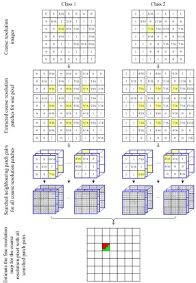
Fig. 3. An example of the fine resolution land cover map estimation procedure, where the coarse resolution patch size is 3. Two land

cover classes are included. For one pixel, all relative coarse resolution patches are extracted for the input fraction images for each

class. The neighboring patch pairs are selected from the training database for each exacted coarse resolution patch. All selected

patch pairs are then used to estimate the resultant fine resolution land cover map, which shows the distribution of the classes and is

still in correct proportion in the input fraction images (9/16 and 7/16, respectively).

E. Estimating the fine spatial resolution land cover map

The fundamental assumption of the proposed learning based SRM algorithm is that coarse spatial resolution

patches with similar class fraction values have similar fine spatial resolution land cover patterns. In order to

estimate the latent fine spatial resolution land cover map, the proposed SRM algorithm aims to make the fine

resolution patches identified from the selected neighboring training patch pairs. Therefore, the objective of the

SRM is to obtain a minimal difference between the fine spatial resolution patch in the estimated fine spatial

resolution land cover map and corresponding fine spatial resolution patches in the neighboring training patch

pairs. During the estimation process, all coarse spatial resolution pixels in the input fraction images are handled

simultaneously, and SRM can be addressed by using the following minimization optimization model:

µ

µ

, ,

, , _,

1 1 1

( ) ( ) ( , )

i

k C M N

i j i j i L T c T c _{H c} c i j

Min  H w x E x x



  



  

µ µ

, , 2

, , , ,

1

1

( , ) ( ( ) ( ))

z p z p

i j i i j i

T c H c T c H c

v

E x x I v I v

z p z p

  



 

  



µ

, , ,

, , , , ,

( i j) 1 ( i j, i ) 1 ( i j, i ) L T c T c H c T c F c

w x   f y y   f y y (7)

Subject to

µ, 1

( ) 1 C H c c I v  



µ µ

2 , ( ) , ( )

H c H c v V

I v f V z



 



where µH is the fine spatial resolution land cover map that we aim to estimate. Setting the coarse spatial

resolution patch size to be odd without loss of generality, i_, F c

y is the coarse spatial resolution patch in which the

th

i coarse spatial resolution pixel is located in the patch center in the fraction images F. Note that i_, F c

y is the

same as _µ,i H c

y because the values in F are preserved in µH as (1). _µ,i H c

x is the corresponding fine spatial

resolution patch of _µ,i H c

y in µH for the class c. , , 1

{ i j}ki

T c j

x _ are fine spatial resolution patches corresponding to

the coarse spatial resolution patches , , 1

{ i j}ki

T c j

y _ in the selected neighboring training patch pairs. ( ,, , µ, )

i j i T c H c E x x is

the difference between two fine spatial resolution patches, _µ,i H c

x and , ,

i j T c

x , and is computed as (6), where

µ, ( )

i H c

I v is the indictor of the fine spatial resolution pixel v within _µ,i H c

x , and , , ( )

i j T c

I v is the indicator of the fine

spatial resolution pixel v within , ,

i j T c

x , respectively. , ,

( i j) L T c

w x is the weight value assigned to the fine spatial

resolution patch , ,

i j T c

x , and is computed in the coarse spatial resolution scale by comparing the fraction difference

weight value. Moreover, Equation (8) ensures that each fine spatial resolution pixel is assigned one and only one

land cover class, and Equation (9) is the area constraint provided by the input coarse spatial resolution fractions

for all coarse spatial resolution pixels.

The minimization problem has a large solution space, which increases with the number of neighboring fine

spatial resolution patches, land cover classes, and the image size. To solve the problem within a short

computational time, this work used a simulated annealing algorithm to find the solution. A power-law annealing

schedule is used in the simulated annealing algorithm [59], where the temperature Tem_n at iteration n is

modified according to

1

n n

Tem   Tem_ (10)

where  (0,1) controls the decrease rate of temperature Tem_n.

In the initialization step, the fine spatial resolution pixels of each class within each coarse spatial resolution

pixel are randomly labeled according to the input coarse spatial resolution fractions. In this situation, the

constraints in (8) and (9) are naturally satisfied. In each iteration, two fine spatial resolution pixels with different

land cover labels are randomly selected in each coarse spatial resolution pixel. The values are then calculated by

using equation (5) according to the current fine spatial resolution land cover map configuration. If swapping

these two fine spatial resolution pixels decreases the object function value in equation (5), these two fine spatial

resolution pixels are swapped. Otherwise, the swap can only be accepted with a small probability according to

the current temperature in equation (10). The algorithm stops when the previously fixed number of iterations is

achieved.

F. Patch outlier rejection

The above-proposed minimization optimization model should be generally considered as a simple fine

resolution map may be disrupted because of the problem of patch outliers. In general, a fine spatial resolution

patch only corresponds to one coarse spatial resolution patch, and their relationship is shown in equation (3). But

on the contrary, given a coarse spatial resolution patch, many different fine spatial resolution patches can

correspond to it, making SRM be an underestimated inversion problem [28].

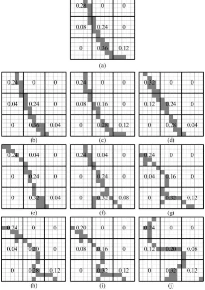
Fig. 4. An example of patch outliers in selected neighboring patch pairs. (a) is a patch pair for one land cover class. The fine

resolution patch includes 15 × 15 pixels and the coarse resolution patch includes 3×3 pixels. The fine resolution pixel filled by grey

color indicates that it belongs to the class. The number within pixels means the area percentages of class in each coarse resolution

pixel of the class. (b) to (j) are searched neighboring patch pairs of (a) using the tolerable fraction difference value. The fraction

values in (b) to (j) are similar with the fraction values in (a), however, only fine spatial resolution patches in (b) and (c) are similar

with that in (a). Fine spatial resolution patches in (g)-(j) are much different with that in (a).

Fig. 4 presents an example of a patch outlier. In Fig. 4(a), a patch pair is taken from an experiment reported

below. This patch pair includes a coarse spatial resolution patch of size 3 × 3, and a fine spatial resolution patch

of size 15 × 15. The numbers within coarse spatial resolution pixels mean the fraction values of the class. Grey

represent the pixels belonging to other classes. Searching in a training database including 120,000 patch pairs by

using the coarse spatial resolution patch in Fig. 4(a) as the reference, the resultant 9 neighboring patch pairs are

simultaneously shown in Figs. 4(b)-(j). As the neighboring patch pairs are searched by comparing the fraction

different between coarse spatial resolution patches, coarse spatial resolution patches in these neighboring patch

pairs are all much similar to the coarse spatial resolution patch in the reference patch pair. When comparing the

fine spatial resolution patches, it is noticed that only fine spatial resolution patches in Fig. 4(b) and Fig. 4 (c) are

very similar with those in Fig. 4(a). Fine spatial resolution patches in Figs. 4(g)-(j) are very different with those

in Fig. 4(a), and are then not suitable to be applied to estimate the fine spatial resolution patch. Therefore, in

order to improve the performance of the learning based SRM algorithm, only the patch pairs which have similar

fine spatial resolution patches with the reference should be applied to estimate the latent fine spatial resolution

land cover map, and other patch pairs should be considered as outliers.

For the fine resolution patch , ,

i j T c

x within the neighboring training patch pairs, it is defined as the outlier

patch according to the following criterion:

, , 2

, , , ,

1

1

( , ) ( ( ) ( ))

z p z p

i j i i j i

T c H c T c H c h

v

f x x I v I v T

z p z p

  



   

  



where ,

, ,

( T ci j, H ci )

f x x

 is the difference between two fine spatial resolution patches, and is computed as same as

, , ,

( i j, i ) T c H c

E x x is equation (6). i_, H c

x is the fine spatial resolution patch in the latent fine spatial resolution land

cover map, and , ,

i j T c

x is the fine resolution patch within the neighboring training patch pairs. The more similar

the fine resolution patches are, the lower the value of , , ,

( i j, i ) T c H c

f x x

 . The threshold T_h is the tolerable difference

between two fine spatial resolution patches. If the value of , , ,

( T ci j, iH c)

f x x

 is no less than that of T_h, the fine

spatial resolution patch , ,

i j T c

x is considered as an outlier patch

.

In the object function (5), , ,

( i j) L T c

w x is used to give the weight values. However, this weight value is

the selected neighboring patch pairs. In order to consider the outlier patches, an additional patch weight

, ,

( i j) H T c

w x that is computed at the fine spatial resolution is added in the object function of the proposed SRM

algorithm as:

µ

µ

, , ,

, , , ,

1 1 1

( ) ( ) ( ) ( , )

i

k C M N

i j i j i j i L T c H T c T c H c c i j

Min  H w x w x E x x



  



  

,

, , ,

,

0 If ( , ) , the patch is an outlier ( )

1 Otherwise, the patch is not an outlier i j i

i j T c H c h H T c

f x x T

w x    

 (13)

In general, if the patch , ,

i j T c

x is an outlier, the weight value , ,

( i j) H T c

w x is set to be zero, meaning that this

fine spatial resolution patch no longer used during the estimation procedure. Otherwise, the weight value

, ,

( i j) H T c

w x is set to be one, if the patch is not the outlier.

Fig. 5. The flowchart of the iterative patch outlier handling procedure.

Setting an appropriate value of Th is important if patch outliers are to be addressed effectively. In the

present work, an iterative method is used. The main iteration procedure is shown in Figure 5. At first, a fine

spatial resolution land cover map is estimated according to the minimization optimization model (5), using all

searched neighboring learning patch pairs. Because all neighboring patch pairs are searched by using a tolerant

the latent fine spatial resolution land cover map. Then, we begin to refine the estimated fine spatial resolution

land cover map, by decreasing the value of T_h step by step, from the maximal threshold Max h

T to the minimal

threshold Min h

T . With each value of Th, a new fine spatial resolution land cover map is estimated according to

(12). At the beginning, with a large T_h value, only a relatively small amount of neighboring patches, whose fine

spatial resolution patches are markedly different to the current estimated fine spatial resolution land cover map,

are considered as outlier. Without these patch outliers, a more accurate fine spatial resolution land cover map is

expected to be estimated. The value of T_h decreases iteratively and more patches are considered as outliers.

Then, the estimated fine spatial resolution land cover map is expected to be more accurate. At the end, the

iteration converges to a stable solution until the minimal value Min h

T is reached, and the estimated fine spatial

resolution land cover map is considered as the result of SRM.

G. The proposed algorithm

According to the aforementioned principles, we summarize the proposed learning based SRM algorithm in

Algorithm 1. In brief, a fine spatial resolution land cover map is first randomly generated using input coarse

spatial resolution fraction images in the initialization step. Meanwhile, the patch pairs in the training database are

constructed according to the zoom factor and the coarse spatial resolution patch size. The input coarse spatial

resolution fraction images are then scanned and neighboring patch pairs are searched by the K-D tree algorithm,

for all coarse spatial resolution patches in fraction images class by class. Using these searched neighboring patch

pairs, the initial fine spatial resolution land cover map is estimated by using the simulated annealing algorithm.

Outliers in these neighboring patch pairs are then found and the fine spatial resolution land cover map is

re-estimated, by changing the threshold value Th. Once Th reaches Min h

T , the iteration is finished, the estimated

Algorithm I

Objective: Estimate fine spatial resolution land cover map H

Input: Coarse spatial resolution fraction images F, zoom factor z, land cover class number C, coarse spatial resolution patch size p, coarse spatial resolution fraction

threshold T_L, the maximal and minimal fine spatial resolution thresholds T_hMax and

Min h

T , fine spatial resolution threshold change value dT_h, parameters of the simulated

annealing algorithm: Tem₀,  , and Ite.

1. Initialization:

1) For each coarse spatial resolution pixel, calculate the number of fine spatial resolution

pixels for each class as (1);

2) Randomly set class label for all fine spatial resolution pixels using the number as the

constraints;

2. Training database generation

1) Extract fine spatial resolution patches from available land cover maps;

2) Estimate the corresponding coarse spatial resolution patch for each fine spatial resolution

patch and generate patch pairs in the training database;

3. Similar Patch Finding

1) Build the K-D tree for all coarse spatial resolution patches in the training database;

2) Scan F, and extract all coarse spatial resolution patches;

3) Search neighboring patch pairs from the training database for all coarse spatial

resolution patches in F.

4. Generating initial high resolution land cover map

1) Reconstruct µH by minimizing the objective function in (5) using the simulated annealing algorithm.

5. Iterative patch outlier rejection

1) Set T_hT_hMax

2) Do {

[1] Calculate the weight values using current Hµ and T_h, according to (13);

[2] Reconstruct Hµ according to (12);

[3] T_hT_hdT_h;

} Until T_hT_hMin

Result: Output the fine spatial resolution land cover map µH.

III. EXAMPLE

The National Land Cover Database 2001 (NLCD 2001) that shows the land cover for the conterminous

cover map over all 50 US states and Puerto Rico at spatial resolution of 30 m, and is primarily generated from

the unsupervised classification of Landsat Enhanced Thematic Mapper Plus circa 2001 satellite dataset [60]. To

simplify the experiment, the original 16 classes of the NLCD images were converted into simple class scheme

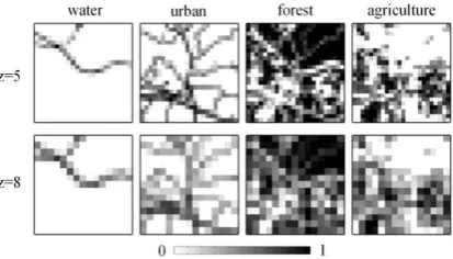
which includes four general land cover classes: water, urban, forest and agriculture.

Fig. 6. All 12 subsets of NLCD land cover maps used to generate the training database. Each subset has 400 × 400 pixels and four

land cover classes.

We select twelve subsets of NLCD maps (each contains 400 × 400 pixels) as shown in Fig. 6 to generate

the coarse and fine spatial resolution patch pairs, which formed the training database. A further four subsets of

NLCD maps (each contains 120 × 120 pixels; Fig.7), were used to assess the proposed SRM algorithm. These

twelve subsets are called as training maps and the four subsets are called as test maps. The locations of these four

test maps are different to those of the twelve training mapsused to construct the training database.For each of

the four test maps, we generate synthetic coarse fraction images by linear averaging the fine spatial resolution

pixel number within the coarse spatial resolution pixel according to different zoom factors. Using simulated

fraction images as input, as well as the constructed training database, the proposed SRM algorithm is applied to

estimate a fine spatial resolution land cover map. In order to assess the accuracy of the proposed learning based

SRM algorithm, by using the test land cover maps as the reference, the overall accuracy (OA) and Kappa

coefficient are used to evaluate the accuracy of the estimated land cover maps, by comparing the entire estimated

map with the corresponding reference map.

The proposed learning based SRM algorithm was also compared with the pixel-based hard classification

method (HC) and several popular SRM algorithms including the pixel swapping algorithm based on simulated

annealing (PS) [61], the sub-pixel/pixel attraction algorithm (SPA) [29], the bilinear interpolation based

algorithm (BI) [56] and the BP neural network based algorithm (BP) [53]. It is noted that the input of PS, SPA

and BI algorithms includes only coarse spatial resolution fraction images, because all these SRM algorithms

describe the land cover distribution using the spatial dependence principle. By contrast, the input of BP

algorithm includes not only the coarse spatial resolution fraction images, but also fine spatial resolution land

cover maps that are used to learn prior land cover information. In the experiments, all twelve training maps are

Fig. 8. Simulated fraction image generated from the test map I as shown in Fig. 7. The top row presents the fraction images at

5

z , and the bottom row presents the fraction images at z8.

The test map I as shown in Fig. 7(a), was first used to assess the impact of parameters in the proposed SRM

algorithm. Synthetic fraction images, as shown in Fig. 8, were simulated from the fine spatial resolution test map

I. Two zoom factors, z5 and z8, were applied. The fine and coarse spatial resolution patch pairs in the

training database were generated from all twelve training maps as shown in Fig. 6 with zoom factors of 5 and 8,

respectively.

When the proposed learning based SRM algorithm is performed, the resultant fine spatial resolution land

cover map is affected by parameters used in the algorithm. According to our experiments, the coarse patch size

p was set to be 3, because a large p value makes the spatial structure of a coarse patch too complex to find

enough similar image patches. Max h

T was set to 1, meaning that no fine spatial resolution neighboring patches

are considered as outliers at the beginning. dT_h was set to 0.05, in order to decrease the value of T_h gradually.

Moreover, to further assess the impact of parameter values on the performance of the proposed method, three

most important parameters including the number of patch pairs in the training database, the coarse spatial

resolution fraction difference threshold value T_L and the minimal fine spatial resolution difference threshold

value Min h

Fig. 9. Kappa values of the resultant fine resolution land cover maps of the proposed learning based SRM algorithm with different

numbers of training patch pairs. (a) is the result at z5; (b) is the result at z8.

1) Impact of the number of patch pairs in the training database: To assess the impact of the number of

patch pairs in the training database, the analysis was repeated 8 times over the range of _{[1 10 , 15 10 ]} 4  4 _{with an}

interval of 4

2 10 . Fig. 9 indicates the Kappa values of resultant fine spatial resolution land cover maps

produced by the learning based SRM algorithm with different numbers of patch pairs in the training database, at

zoom factors of 5 and 8, respectively. When the number is less than _{3 10} 4_{, the Kappa values of the results at}

5

z and z8 are both at a low level. This is because the use of only a few patch pairs cannot provide

enough information about the spatial land cover patterns. With the increment of the number, both Kappa values

at z5 and z8 increase rapidly until the number reaches to about 4

11 10 , and then the Kappa values

maintain stable, as shown in Figs. 9 (a) and (b). It is also noticed that the increment of Kappa values at z5 is

more rapid than that at z8, when the number is in the range of 4 4

[3 10 , 9 10 ]  . The reason is that more patch

pairs are needed in order to decrease the uncertainty caused by a large zoom factor. According to the experiment,

a number of patch pairs larger than 4

11 10 is reasonable. As more patch pairs may increase the calculation

burden, the number of patch pairs in the training database is set to be 4

12 10 in our latter experiments.

2) Impact of the threshold T_L: The threshold value T_L is a pre-defined parameter that represents the

tolerable fraction difference between two coarse spatial resolution patches. This parameter guarantees that the

searched coarse spatial resolution patch which has a fraction difference f larger than T_L cannot be accepted

maps produced by the proposed learning-based SRM algorithm with different T_L values. When T_L is in the

range of [0.02, 0.14] at z5 and in the range of [0.02, 0.12] at z8, the Kappa values increase with the

increment of the value of T_L. This is because that the number of candidate patch pairs is too small to provide

enough land cover pattern information for SRM, if T_L is set to be a too low value. For z5, as shown in Fig.

10(a), if the value of T_L is larger than 0.14, the Kappa values are kept at a stable level. For z8, however, the

Kappa values begin to decrease until a stable value, if T_L is larger than 0.12. In general, with a larger value of

L

T , more patch pairs with larger fraction errors are considered as candidate patches, which indeed generally

provide erroneous information and make the estimated fine spatial resolution land cover map differ significantly

from the latent map. Setting too large a value of T_L may degrade the estimated fine spatial resolution map.

However, the result is only slightly different because of the additional patch outlier rejection procedure.

Fig. 10. Kappa values of the resultant fine resolution land cover maps of the proposed learning based SRM algorithm with different

values of coarse resolution threshold T_F. (a) is the result at z5; (b) is the result at z8.

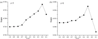
Fig. 11. Kappa values of the resultant fine resolution land cover maps of the proposed learning based SRM algorithm with different

minimal fine resolution threshold T_hMin. (a) is the result at z5; (b) is the result at z8.

3) Impact of the minimal fine spatial resolution threshold of Min

h

T : The value of Min h

T is denoted as the

estimation procedure. To assess the impact of the Min h

T value, the learning based SRM algorithm was applied

with different values of Min h

T in the range of [1.0, 0.1] with an interval of -0.1. The Kappa values of the

resultant fine spatial resolution land cover maps produced by the proposed learning based SRM algorithm at

5

z and z8 are shown in Fig. 11. With the decrement of the values of Min h

T , the corresponding Kappa

values of the resultant fine spatial resolution land cover maps increase, because more coarse spatial resolution

patches are considered as outlier patches and not used in the estimation procedure. When Min h

T is larger than 0.2

at z5 and 0.3 at z8, however, the Kappa values begin to decrease as the value of T_h decreases. The

reason is that most neighboring patches are considered as outliers if the value of T_h is too low, and the

remaining neighboring patches can not provide enough information for SRM.

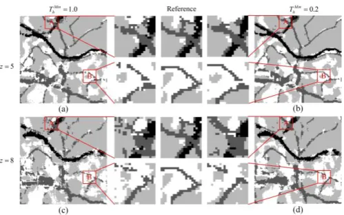
Fig. 12. Resultant fine resolution land cover maps produced by the proposed learning based SRM algorithm. (a) is the result without

patch outlier handling procedure and (b) is the result using patch outlier handling procedure at z5. (c) is the result without

patch outlier handling procedure and (d) is the result using patch outlier handling procedure at z8. Using the patch outlier

handling procedure reduces the salt-and-pepper artifacts as shown in the enlarged part A, and the linear discontinuities as shown in

the enlarged part B.

A visual comparison, as shown in Fig. 12, is used to further assess the impact of the value of Min h

T . For

5

z , as shown in Fig. 12(a), many salt-and-pepper artifacts appear and the spatial continuities of some linear

features are interrupted when Min 1.0 h

T  , which means that all patches are accepted and no outliers exist. In

contrast, with patch outlier rejection (when Min 0.2 h

the spatial continuities are well maintained, as shown in Fig. 12(b). The impact of Min h

T on the resultant fine

spatial resolution land cover map is more obvious when z8. Many salt-and-pepper artifacts and linear

discontinuities that appear in the fine spatial resolution land cover map, as shown in Fig. 12(c), are eliminated by

the outlier rejection, as shown in Fig. 12(d).

Fig. 13. Resultant land cover maps generated by different methods with z5 and z8 for the test map I. HC produces jagged

boundaries (such as the area A); PS produces isolated patches (such as the area B); SPA and BI produce linear artifacts (such as the

area C); and BP produces salt-and-pepper artifacts and isolated patches (such as the area D).

4) Comparison with other methods: According to aforementioned discussion about parameters used in the

proposed learning based SRM method, the optimal parameter values were used to produce the resultant fine

spatial resolution land cover maps. In particular, the number of patch pairs in the learning database is 4

12 10 ,

the value of Tf is 0.12 , and the value of Min h

T is 0.2 for z5 and 0.3 for z8, respectively. By using the

same aforementioned simulated coarse fraction images used for the proposed learning based SRM method as

input, the resultant land cover maps of HC, PS, SPA, BI, BP and the proposed learning based SRM are all shown

in Fig. 13. Additionally, the Kappa and OA values of all these maps produced by different methods are shown in

Table I.Kappa and Overall Accuracy (OA) values of the resultant land cover maps produced by different methods at z5 and

8

z for the test map I.

HC PS SPA BI BP Proposed

z=5

Kappa 0.6223 0.6525 0.6780 0.6856 0.7050 0.7348

OA 0.7735 0.7890 0.8045 0.8091 0.8209 0.8390

z=8

Kappa 0.4811 0.4739 0.5068 0.5148 0.5264 0.5561

OA 0.6957 0.6806 0.7006 0.7054 0.7124 0.7305

In general, for all SRM algorithms, the zoom factor plays an important role on the accuracy of result. The

key point of SRM is to determine the class labels of the fine spatial resolution pixels within the coarse spatial

resolution pixel. For a given zoom factor z, there will be z z fine spatial resolution pixels within the coarse

spatial resolution pixel to be estimated. With the increase of z, the number of fine spatial resolution pixels

would be increased exponentially, and more fine spatial resolution pixels within the coarse spatial resolution

pixel need to be estimated. Therefore, the uncertainty of the estimation would be expected to increase, and the

performance of the algorithm would decrease.

For the results of HC, as shown in Fig. 13 and Fig. 13, the land cover boundaries are jugged and many

spatial details are missed. The Kappa and OA values of the results of HC, as shown in Table. I, stay at the lowest

level. This is because that HC is based on the pixel scale, and does not consider the spatial distribution of classes

at sub-pixel scale. By contrast, more land cover details at the sub-pixel scale are maintained by SRM including

PS, SPA, BI, BP and the proposed learning-based SRM method. Visual comparison of the fine spatial resolution

maps obtained from the various SRM analyses highlighted differences in the way they represented the land cover.

For the results of PS, many land cover features are mapped as isolated rounded patches, and the spatial

When z8, the Kappa and OA values of PS are 0.4739 and 0.6806, and are even lower than those of HC

because the uncertainty of the fine spatial resolution pixel distributions in the resultant fine spatial resolution

land cover map generated by PS is serious when the zoom factor is large. The fine spatial resolution land cover

maps produced by SPA and BI visually differed from that obtained with PS with more spatial detail are

maintained. The Kappa and OA values of fine spatial resolution land cover maps produced by SPA and BI are

also higher than those of PS. However, numerous linear artifacts are found near the land cover boundaries in the

obtained fine spatial resolution land cover maps produced by SPA and BI, and the linear artifacts become more

serious with the increment of the zoom factor. The fine spatial resolution land cover maps produced by PS, SPA

and BI are, therefore, less than ideal. This is because these SRM methods just apply the spatial dependence

assumption to describe the land cover pattern, and this assumption will often be too simple to provide enough

information for SRM in areas with complex land cover patterns.

Compared with the results of PS, SPA and BI, the linear artifacts in the results of BP are eliminated and the

spatial continuities are maintained to some extent. The Kappa and OA values of the resultant fine spatial

resolution land cover maps produced by BP at zoom factor of 5 and 8 are both higher than those of PS, SPA and

BI. This improvement arises from the use of additional information about the spatial land cover pattern that is

learned from the training database in the SRM procedure. However, in the resultant fine spatial resolution land

cover maps produced by BP, many salt-and-pepper artifacts are found and many linear land cover features are

also mapped as isolated small-sized patches. Moreover, with the increment of the zoom factor, the geometric

integrity of features is more difficult to be maintained by the BP based SRM method. The shortcoming of the BP

based SRM method is mainly caused by its two-step procedure and the impact of outliers during the learning

procedure.

are more similar to the reference (Fig. 7) at both zoom factors than the maps produced from the other SRM

methods. Isolated land cover patches, jagged shapes and linear artifacts, which are common in the resultant fine

spatial resolution land cover maps produced by aforementioned methods, are effectively eliminated by the

proposed learning based SRM method. More spatial details, especially the linear features and the spatial land

cover continuities are maintained. The Kappa and OA values of the resultant fine spatial resolution land cover

maps produced by the proposed learning based SRM method are all the highest at both zoom factors.. Both the

visual comparison and accuracy analysis indicate that the proposed learning-based SRM method is superior to

the SRM algorithms used for comparison.

The test maps II to IV, as shown in Figs. 7(b) to (d), were used to further validate the performance of the

proposed learning-based SRM method. As with the analyses focused on test map I, with the zoom factors of 5

and 8, the three fine spatial resolution test maps were degraded to produce the simulated coarse spatial resolution

fraction images. These simulated coarse spatial resolution fraction images are then used as input to the SRM

methods in order to produce the resultant fine spatial resolution land cover maps. The same parameter values

used in the experiment of the test map I were applied for test maps II to IV. The resultant land cover maps

produced by HC, PS, SPA, BI, BP and the proposed learning based SRM algorithm at zoom factors of 5 and 8

are all shown in Fig. 14 and Fig. 15, respectively. By using the original fine spatial resolution land cover maps as

the reference, the accuracy analysis of three land cover maps at z5 and z8 are shown in Table II.

A similar trend as the experiment of the test map I is found by visually comparing the resultant fine spatial

resolution land cover maps produced by different methods. The resultant land cover maps produced by HC have

jagged boundaries and many spatial details are missed. By contrast, the fine spatial resolution land cover maps

produced by SRM methods have smooth boundaries and more spatial details are maintained. The fine spatial

into individual round patches for all three test maps. The spatial land cover pattern of the results produced by

SPA and BI are much improved, however, numerous irregular linear artifacts exist near the boundaries.

Moreover, more linear artifacts appear in the SPA and BI results of the test map III than those of the test map II

and IV, due to the complex land cover features of the test map III, especially the urban class. The BP based SRM

method can reconstruct more spatial details, and eliminate linear artifacts in the results of SPA and BI to some

extent, due to additional spatial land cover information is learned from the extra fine spatial resolution land cover

maps. However, many salt-and-pepper artifacts and isolated small-sized patches are still unavoidable due to the

errors caused by the two-step process. By contrast, the fine spatial resolution land cover maps produced by the

proposed learning-based SRM method, as shown in Fig. 14 and Fig. 15 at z5 and z8, are more similar to

the reference fine spatial resolution land cover maps as shown in Fig. 7. The fine spatial resolution land cover

maps produced by the proposed algorithm are smooth. Salt-and-pepper artifacts, isolated patches and irregular

linear artifacts that appear in the results of some of the other SRM analyses are mostly eliminated. For all of the

three testing land cover maps at both zoom factors of 5 and 8, more spatial detail, especially the linear features,

Fig. 14. Resultant land cover maps generated by different methods for test maps II-IV with z5. HC produces jagged boundaries

(such as the area A); PS produces isolated patches (such as the area B); SPA and BI produce linear artifacts (such as the area C); and

BP produces salt-and-pepper artifacts and isolated patches (such as the area D).

Fig. 15. Resultant land cover maps generated by different methods for test maps II-IV with z8. HC produces jagged boundaries

(such as the area A); PS produces isolated patches (such as the area B); SPA and BI produce linear artifacts (such as the area C); and

BP produces salt-and-pepper artifacts and isolated patches (such as the area D).

Table II.Kappa and Overall Accuracy (OA) values of the resultant land cover maps produced by different methods at z5 and

8

z for test maps II-IV.

HC PS SPA BI BP Proposed

Test map II z=5

Kappa 0.6576 0.7157 0.7466 0.7392 0.7465 0.7790

OA 0.8126 0.8381 0.8556 0.8514 0.8556 0.8741

z=8

Kappa 0.5746 0.5770 0.6190 0.6232 0.6230 0.6441

OA 0.7690 0.7590 0.7829 0.7853 0.7852 0.7972

Test map III z=5

Kappa 0.6006 0.6273 0.6547 0.6453 0.6596 0.6939

OA 0.7481 0.7599 0.7776 0.7715 0.7808 0.8028