Nonlinear frequency conversion in isotropic semiconductor waveguides

SEMICONDUCTOR WAVEGUIDES

Konstantinos Moutzouris

A Thesis Submitted for the Degree of PhD

at the

University of St Andrews

2003

Full metadata for this item is available in

St Andrews Research Repository

at:

http://research-repository.st-andrews.ac.uk/

Please use this identifier to cite or link to this item:

http://hdl.handle.net/10023/13117

in Isotropic Semiconductor

Waveguides

Konstantinos Moutzouris

A thesis submitted to the University of St Andrews in

application for the degree of Doctor of Philosophy

This thesis describes an experimental investigation of optical frequency conversion in isotropic semiconductor waveguides by use of several phase-matching approaches.

Efficient, type I second harmonic generation of femtosecond pulses is reported in birefringently-phase-matched GaAs/Alox waveguides pumped at 2.01 µm. Practical second harmonic average powers of up to ~ 650 µW are obtained, for an average launched pump power of ~ 5 mW. This corresponds to a waveguide conversion efficiency of ~ 20 % and a normalized conversion efficiency of greater than 1000 % W-1cm-2. Pump depletion of more than 80 % is recorded.

Second harmonic generation by type I, third order quasi-phase-matching in a GaAs-AlAs superlattice waveguide is reported for fundamental wavelengths from ~1480 to 1520 nm. Quasi-phase-matching is achieved through modulation of the nonlinear coefficient , which is realised by periodically tuning the superlattice bandgap. An average output power of ~25 nW is obtained for a launched pump power of <2.3 mW.

) 2 (

zxy

χ

Type I second harmonic generation by use of first order quasi-phase-matching in a GaAs/AlAs symmetric superlattice waveguide is also reported, with femtosecond fundamental pulses at 1.55 µm. A periodic spatial modulation of the bulk-like second-order susceptibility χ_zxy(2) is realized using quantum well intermixing by As+ ion implantation. A practical second harmonic average power of ~1.5 µW is detected, for a coupled pump power of ~11 mW.

Second harmonic generation through modal-phase-matching in GaAs/AlGaAs semiconductor waveguides is reported. Using femtosecond pulses, both type I and type II second harmonic conversion is demonstrated for fundamental wavelengths near 1.55 µm. An average second harmonic power of ~10.3 µW is collected at the waveguide output for a coupled pump power of <20 mW.

I, Konstantinos Moutzouris, hereby certify that this thesis, which is approximately 55000 words in length, has been written by me, that it is the record of work carried out by me and that it has not been submitted in any previous application for a higher degree.

Konstantinos Moutzouris September 2003

I was admitted as a research student in September 1999 and as a candidate for the degree of Doctor of Philosophy in September 1999; the higher study for which this is a record was carried out in the University of St. Andrews between 1999 and 2003.

Konstantinos Moutzouris September 2003

I hereby certify that the candidate has fulfilled the conditions of the Resolution and Regulations appropriate for the degree of Doctor of Philosophy in the University of St. Andrews and that the candidate is qualified to submit this thesis in application for that degree.

Dr. Majid Ebrahimzadeh September 2003

In submitting this thesis to the University of St. Andrews I understand that I am giving permission for it to be made available for use in accordance with the regulations of the University Library for the time being in force, subject to any copyright vested in this work not being affected thereby. I also understand that the title and abstract will be published, and that a copy of the work may be made and supplied to any bona fide library or research worker.

First and foremost, I wish to thank my supervisor throughout this work, Dr Majid Ebrahimzadeh, for his guidance, insight and enthusiasm. For his support and encouragement I am greatly indebted.

My thanks are also due to the rest of the St. Andrews SCNLO group members, for their vital contribution to this work. That is, in a chronological order, to: Tom Brown

(who introduced me to the world of experimental optics), Soma Venugopal Rao (who worked on this project for the greatest part of it), as well as the new “additions” to the group, Abdul, Masood and Reza (to all of whom I wish the best in continuing this work).

Many thanks also to our collaborators from Paris, Glasgow, and Rome. Not only for contributing their expert knowledge in designing and fabricating nonlinear waveguides, but also because it was a great pleasure to work with all of them! From a long list of names, I would like to specially thank Alfredo De Rossi, Vincent Berger, Amr Saher Helmy, Khalil Zeaiter, Todd Kleckner, Daniele Modotto, David Hutchings, and Giuseppe Leo.

Thanks also to a number of people in the school (staff and students) for their help and support. In particular, I wish to thank Ian Lindsay, David Stothard, Tom Edwards,

Arvydas Ruseckas, Pablo Alvarez, Ben Agate, Michael Spurr, Andrew Woodman,

Jonathan Phillips, Julia Fenn, Veneranda Garces-Chavez, Edik Rafailov and Aly Gillies, as well as, of course, the secretary Mary Rodger and the legendary workshop staff, George Radley and Paul Aitken!

Many thanks to my friends in St Andrews, people like Kostas (Petridis), Yannis

(Tsapras), Lefteris, Vivi, Tomas, Yannis (Tellidis), Eva, Petros, Kostas

(Yannopoulos), Kostas (Papathanassiou), Irene, Yannis (Markouris), Valia,

Vaggelis…

Many thanks also to Agapitos Roukounakis, for causing all this.

Last but not least, thanks to Katrin.

Thanks to Yannis and Maria.

Abstract...I Declarations... II Copyright Declarations...III Acknowledgements...IV Table of Contents... V

1. Prologue

Reference ... 5

2. Nonlinear Optics Concepts

2.1 Review of Maxwell equations ... 7

2.2 On the optical polarisation of matter ... 12

2.2.1 The anharmonic oscillator treatment of the optical polarisation ... 12

2.2.2 Nonlinear susceptibility ... 16

2.3 Propagation of electromagnetic waves in nonlinear media ... 20

2.3.1 Coupled wave equations for nonlinear frequency conversion... 20

2.3.2 The Manley-Rowe relations... 22

2.3.3 Second order nonlinear frequency conversion processes and gain... 23

2.4 Phase-matching ... 27

2.4.1 The physical content of phase-matching ... 27

2.4.2 Birefringent-phase-matching (BPM) ... 29

2.4.3 Quasi-phase-matching (QPM) ... 34

2.4.4 Phase-matching acceptance bandwidths ... 38

2.5 Nonlinear interactions with Gaussian beams ... 40

2.6 Summary ... 42

References... 43

3. Femtosecond Optical Parametric Oscillator... 46

3.1 Introduction... 46

3.2 Synchronously pumped optical parametric oscillators ... 47

3.2.1 Optical parametric devices: An overview... 47

3.2.2 Steady-state analysis of the continuous wave, singly resonant OPO.... 48

3.2.3 SPO spectral considerations... 51

3.2.4 SPO temporal considerations... 52

3.3.2 Device configuration and alignment ... 58

3.3.3 Device performance ... 61

3.4 Conclusions... 66

References... 67

4. Efficient Second Harmonic Generation in Birefringently-

Phase-Mathced GaAs/Al

O

Waveguides

4.1 Introduction... 70

4.2 Birefringent-phase-matching technologies in isotropic materials ... 71

4.2.1 Form birefringence in a laminar structure ... 71

4.2.2 Phase-matching by use of form birefringence ... 74

4.3 Optical experiment... 76

4.3.1 Sample details ... 76

4.3.2 Experimental set-up ... 78

4.3.3 Results and discussion ... 80

4.3.4 Efficiency considerations... 87

4.4 Conclusions... 89

References... 90

5.

Second Harmonic Generation in Quasi-Phase-Matched

GaAs/AlAs Waveguides

5.1 Introduction... 92

5.2 Quasi-phase-matching technologies in III-V semiconductors... 93

5.2.1 Quantum-well intermixing (QWI) ... 93

5.2.2 Quasi-phase-matching strategies by use of QWI... 98

5.3 Initial efforts: Third order quasi-phase-matching experiment ... 101

5.3.1 Sample details and experimental set-up... 101

5.3.2 Results and discussion ... 104

5.4 Optimised design: First order quasi-phase-matching experiment ... 107

5.4.1 Sample details and experimental set-up... 107

5.4.2 Results and discussion ... 109

5.5 Conclusions... 113

Using Modal-Phase-Matching

6.1 Introduction... 116

6.2 Modal-phase-matching schemes in semiconductor waveguides ... 117

6.2.1 Modal-phase-matching principles: The case study of the slab waveguide... 117

6.2.2 M-type waveguides for efficient nonlinear frequency conversion ... 120

6.3 Optical experiment... 123

6.3.1 Sample details ... 123

6.3.2 Experimental set-up ... 125

6.3.3 Results and discussion ... 126

6.4 Conclusions... 134

References... 135

7. Optical Loss Analysis in Semiconductor Waveguides

7.1 Introduction... 137

7.2 Development of a femtosecond scattering technique for transmission loss measurements ... 138

7.2.1 Operating principles and experimental set-up ... 138

7.2.2 Results and discussion ... 140

7.2.3 Nonlinear loss studies ... 146

7.3 Conclusions... 148

References... 149

8. General Conclusions

8.1 Summary of results ... 151

8.2 BPM, QPM, MPM: A comparative discussion... 155

8.3 Future work... 164

References... 165

Appendix A: Ultrashort Pulse Considerations

A.1 Pulse propagation... 168

A.2 Group velocity dispersion compensation... 173

A.3 Pulse duration measurements... 174

1. Prologue

The present thesis outlines work carried out at the University of St. Andrews during the period 1999-2003, in the area of nonlinear frequency conversion in III-V semiconductor waveguides. This work was performed within the frame of an ongoing European collaboration (OFCORSE project1), which comprised four participant members2. The objective of this collaboration is to exploit the optical nonlinearities in III-V semiconductor materials for efficient nonlinear frequency conversion. This could lead to the development of numerous functional devices operating in the near and mid-infrared (IR), ranging from second harmonic generation structures, to integrated devices for difference frequency generation, parametric amplification and oscillation.

Accessing the near and mid-IR spectral region is of considerable interest for a number of applications. Most molecules present vibrational resonances within the 2 to 20 µm wavelength range [1], making compact sources in the near and mid-IR imperative for spectroscopic studies [2,3], as well as for gas sensing purposes with potential use in environmental monitoring [4,5] and photo-medicine [6]. Furthermore, generation and conversion of coherent radiation at 1.55 µm could be useful for applications in wavelength division multiplexing and all-optical switching in telecommunication networks [7-9]. Nonlinear frequency conversion in this spectral range has also been proposed as a route to designing twin-photon sources for quantum optical communications [10] and for testing fundamental concepts of quantum physics and relativity [11].

Current infrared laser sources include narrow-band laser diodes [12], lead salt [13] and antimonide lasers [14]. In general these approaches require cryogenic cooling, offer modest output powers and do not produce a tunable output. A novel addition to the family of infrared sources is the quantum cascade laser [15], which is still

1

Optical Frequency COnveRsion in Semiconductors

2

1) The group of Prof. Assanto at Roma University-III, which focused on theoretical studies, 2) The group of Prof. Berger at Thomson CSF (THALES), which was responsible for the design and fabrication of birefrintent materials,

3) The group of Prof. Aitchinson at Glasgow University, which concentrated its efforts on designing and fabricating quasi-phase-matched structures, and

undergoing intense development. Available quantum cascade lasers offer high output power levels and considerable temperature tuning, yet continuous-wave, room temperature operation has been proven illusive. Sources based on nonlinear frequency conversion (most notably, the optical parametric oscillation and difference frequency generation) represent an attractive alternative to accessing this spectral region [1, 4, 5, 16]. Efforts in this direction have been mostly focused on the search for materials with the desirable properties. Unquestionably, the most promising breakthrough in nonlinear material science and fabrication technology followed the development of periodically polled lithium niobate [17]. However, the transparency range of lithium niobate limits its use to wavelengths shorter than ~5 µm. Other infrared materials developed to date, such as chalcopyrites [18], still suffer from a variety of issues related to the immature growth technologies available.

In this direction, GaAs/AlGaAs emerges as a very attractive infrared nonlinear material system for a number of reasons. First and foremost, GaAs exhibits a large second order nonlinearity with reported values for the second order nonlinear coefficient d14=d36 of ~100 pm/V in the IR [19-23]. This value is approximately three times higher than the respective value for lithium niobate and two orders of magnitude larger than that of conventional birefringent materials. Further distinctive advantages of this material include its broad IR transparency (0.9-17 µm), low optical absorption, high damage threshold, high thermal conductivity and mature growth and fabrication technology, which supports the possibility of integration with semiconductor laser sources as well as the potential for mass production at low cost. On the negative side, GaAs has a cubic symmetry and thus is optically isotropic and lacks natural birefringence. Therefore, matching the phase velocities of the interacting waves (a necessity for efficient frequency conversion) is not a straightforward process. Circumventing the problem of phase-matching has been the principal challenge of this project. Three different phase-matching approaches have been proposed and studied:

• Artificial (or form) birefringence, by means of selective oxidation

• Quasi-phase-matching, through quantum well intermixing, and

Within the broader framework of the OFCORSE project, scope of the present doctoral work was to investigate the feasibility of the preceding phase-matching techniques through investigations of second harmonic generation in guided-wave GaAs-based structures. The waveguide-based design yields the high intensities and provides maximised overlap between the interacting modes that are necessary for high conversion efficiencies. The significance of such a study is three-fold: Firstly, it is a step towards the establishment of GaAs as a practical nonlinear material. Secondly, it demonstrates a hybrid frequency converter with its own, independent significance. Thirdly, it serves as a guideline for the further development of integrated devices.

For this purpose, the early efforts were directed towards setting up a complete characterisation facility. A synchronously pumped, femtosecond optical parametric oscillator (OPO) was constructed and served as the pump source. The OPO was a reasonable choice, since it provides a unique wavelength tuning capability, which is necessary to overcome unavoidable inaccuracies and errors in the prediction of the phase-matching wavelength. Operation in the femtosecond regime was favoured in order to achieve the large peak powers necessary for efficient conversion. The laboratory was also equipped with a number of commercial instruments, including optic elements, end-fire coupling apparatus, IR cameras, microscopes and detection diagnostics.

This thesis is organised in eight chapters. The present (first) chapter provides a short introduction to the scope and challenges of this project. The second chapter summarises basic concepts of nonlinear optics that are fundamental to this work. The third chapter is dedicated to presenting an overview of the femtosecond optical parametric oscillator that was constructed and used as the main experimental tool for the material characterisation. The three following chapters present details of the different approaches used to solve the phase velocity synchronism problem, along with results from the corresponding harmonic generation experiments, namely: Phase- matching based on form firefringence (fourth chapter), quasi-phase-matching (fifth chapter) and modal-phase-matching (sixth chapter). The seventh chapter reports results from measurements of the propagation loss on these materials based on a femtosecond scattering technique. The thesis concludes with a summary and a comparison of the results, which is attempted in the eighth chapter. Finally, two appendices are included to discuss special issues on ultrashort pulse propagation and measurement (appendix A), and list the publications arising from this work (appendix B).

It should be mentioned that throughout these years a number of further experiments was carried out, including:

• Investigation of parametric oscillation based on a LiInS2 crystal,

• Demonstration of optical rectification in GaAs waveguides, and

• Generation of femtosecond blue light pulses through frequency doubling in a BiBO crystal.

References

[1] K. Fradkin, A. Arie, A. Skliar, and G. Rosenman, Tunable mid-infrared source by

difference frequency generation in bulk periodically poled KTiOPO4, Appl. Phys. Lett. 74,

914, (1999)

[2] R.F. Curl, F.K. Tittel, Tunable infrared laser spectroscopy, Annu. Rep. Prog. Chem. Sel C 98, 217, (2002)

[3] L. Windhorn, T. Witte, J.S. Yeston, D. Proch, M. Motzkus, K.L. Kompa, and W. Fuss,

Molecular dissociation by mid-IR femtosecond pulses, Chem. Phys. Lett. 357, 85, (2002)

[4] Y. Mine, N. Melander, D. Richter, D.G. Lancaster, K.P. Petrov, R.F. Curl, and F.K. Tittel,

Detection of formaldehyde using mid-infrared difference frequency generation, Appl. Phys. B

65, 771, (1997)

[5] K.P. Petrov, A.T. Ryan, T.L. Patterson, L. Huang, S.J. Field, and D. J. Bamford, Mid-infrared spectroscopic detection of trace gases using guided-wave difference frequency

generation, Appl. Phys. B 67, 357, (1998)

[6] W. Petrich, Mid-infrared and Raman spectroscopy for medical diagnostics, Appl. Spectr. Rev. 36, 181, (2001)

[7] S.J.B. Yoo, Wavelength conversion technologies for WDM network applications, IEEE J. Lightwave Tech. 14, 955, (1996)

[8] C.G. Trevino-Palacios, G.I. Stegeman, P. Baldi, and M.P.D. Micheli, Wavelenght shifting

using cascaded second order processes for WDM applications at 1.55 .µm, Electron. Lett. 34,

2157, (1998)

[9] G.D. Landry, and T.A. Maldonado, Switching and second harmonic generation using

counterpropagating quasi-phase matching in a mirror-less configuration, J. Lightwave Tech.

17, 316, (1999)

[10] W. Tittel, J. Brendel, N. Gisin, and H. Zbinden, Quantum cryptography using entangled

photosin energy-time Bell states, Phys. Rev. Lett. 84, 4737, (2000)

[11] N. Gisin, J. Brendel, H. Zbinden, A. Sergienko, and A. Muller, Twin photon techniques

for fiber measurements, Proc. Symposium Opt. Fiber Measurements, NIST Boulder Colorado,

35, (1998)

[12] A. Joullie, E.M. Skouri, M. Garcia, P. Grech, A. Wilk, P. Christol, A.N. Baranov, A. Behres, J. Kluth, A. Stein, K. Heime, M. Heuken, S. Rushworth, E. Hulicius, and T. Simecek,

InAs(PSb)-based “W” quantum well laser diodes emitting near 3.3 µm, Appl. Phys. Lett. 76,

2499, (2000)

[13] G.T. Forrest, D. Wall, and J. Oconnell, Recent advances in lead salt laser technology

and the implications for gas-analysis, Proc. Soc. Photo-optical Instrumentation Engineers

461, 2, (1984)

[14] R.M. Biefeld, A.A. Allerman, S.R. Kurtz, E.D. Jones, I.J. Fritz, and R.M. Sieg, The growth of infrared antimonide-based semiconductor lasers by metal-organic chemical vapor

deposition, J. Mater. Science 13, 649, (2002)

[15] F. Capasso, C. Gmachl, R. Paiella, A. Tredicucci, A.L. Hutchinson, D.L. Sivco, J.N.

Baillargeon, A.Y. Cho, and H.C. Liu, New frontiers in quantum cascade lasers and

[16] D. Campi, and C. Cariasso, Wavelength conversion technologies, Photon. Tech. Lett. 2, 85, (2000)

[17] M.M. Fejer, G.A. Magel, and E.J. Lim, Quasi-phase-matched interactions in lithium

niobate, Pros. SPIE 1148, 213, (1998)

[18] M.C. Ohmer, and R. Pandey, eds, Emergence of chalcopyrites and nonlinear optical

materials, Materials Research Bulletin, Special Issue, (1998)

[19] T. Skauli, K.L. Vodopyanov, T.J. Pinguet, A. Schober, O. Levi, L.A. Evers, M.M. Fejer,

J.S. Harris, B. Gerard, L. Becouarn, E. Lallier, and G. Arisholm, Measurement of the

nonlinear coefficient of orientation-patterned GaAs and demonstration of highly efficient

harmonic generation, Opt. Lett. 27, 628, (2002)

[20] C.K.N. Patel, Optical harmonic generation in the infrared using a CO2 laser, Phys. Rev.

Lett. 16, 613, (1966)

[21] D.A. Roberts, Simplified characterisation of uniaxial and biaxial nonlinear optical

crystals – a plea for standardisation of nomenclature and conventions, IEEE J. Quantum

Electron. 28, 2057, (1992)

[22] M.M. Choy, and R.L. Byer, Accurate second order susceptibility measurements of

visible and infrared nonlinear crystals, Phys. Rev. B 14, 1693, (1976)

[23] I. Shoji, T. Kondo, A. Kitamoto, M. Shirane, and R. Ito, Absolute scale of second order

2. NONLINEAR OPTICS CONCEPTS

2.1 Review of Maxwell equations

In 1864, J.C. Maxwell enclosed the fundamental laws governing the generation, propagation and interaction of electromagnetic (EM) radiation with matter, in the famous set of equations (2-1). Expressed in MKSA units, Maxwell equations are:

0 ) , ( ) , ( = ∂ ∂ + ×

∇ B r t

t t r

Er r r r

r (2-1 a) ) , ( ) , ( ) ,

( D r t J r t

t t r

Hr r r r r r

r ₌

∂ ∂ − ×

∇ (2-1 b)

0 ) ,

( =

⋅

∇r Br rr t (2-1 c)

) , ( ) ,

(r t r t

Dr r r

r

ρ

= ⋅

∇ (2-1 d)

where: Er…is the electric field intensity vector in Volts/meter

Hr…is the magnetic field intensity vector in Ampere/meter

Br…is the magnetic flux density vector in Tesla

…is the electric displacement vector in Coulomb/meter

Dr 2

…is the electric current density vector in Ampere/meter

Jr 2

ρ…is the electric charge density in Coulomb/meter3

Er,Hr,Br,Dr,Jr and ρ are real functions of time t and spatial location with respect to a specific coordinate system rr. Solving Maxwell equations to determine the field vectors, requires three relations that reveal the behaviour of the medium under the influence of the field, known as the constitutive relations:

Dr(rr,t)=Dr{Er(rr,t),Hr(rr,t)} (2-2 a) )} , ( ), , ( { ) ,

(r t B E r t H r t

Br r = r r r r r (2-2 b) )} , ( ), , ( { ) ,

(r t J E r t H r t

Jv r = r r r r r (2-2 c) If the field vectors are linearly related, the medium is said to be linear and the constitutive relations take the form:

) , ( ) ( ) , ( ) , ( ) ,

(r t ₀E r t P r t ₀ r E r t

Dr r =ε r r + r r =ε ε r r r (2-3 a) ) , ( ) ( ) , ( ) , ( ) ,

(r t 0H r t M r t 0 r H r t

Br r =µ r r + r r =µ µ r r r (2-3 b) ) , ( ) ( ) ,

(r t r E r t

where:

ε

µ

Pr … is the macroscopically averaged electric dipole (optical polarisation) Mr … is the magnetisation

ε

µ ... is the relative permeability of the medium

σ

If ε, µ and σ are constant through the medium, the medium is said to be homogenous. The medium is referred to as isotropic when ε, µ and σ are scalar quantities. In the proceeding equations, it has been assumed that the polarisation (magnetisation) and the electric (magnetic) field intensity are linearly related, so that one can write:

[

]

) ,

(r t 0 r E r t 0 (1)E r t

Pr r =ε −ε r r r =ε χ r r (2-4) where:

ε

χ(1) =1− (2-5)

is known as the (first order or linear) susceptibility of the medium.

In the rest of this section some main results are outlined in the linear response limit for future reference. The most important consequence arising from Maxwell equations is that they can be formulated in a wave-motion equation and, thus, establish the existence of electromagnetic waves. For a linear, isotropic and homogeneous medium the wave equation derived by use of the standard four-step-process1 has the well-known form: t t r J t t r E t r E ∂ ∂ = ∂ ∂ −

∆ ( , ) ( , ) ₀ ( , )

2 2 0 0 r r r r v r µ µ µ εµ

ε (2-6)

where ∆=∇2denotes the linear vector Laplace operator.

1

(1) From (2-1 a) follows: ( ) 0 ( H)

t

Er r r

r r × ∇ ∂ ∂ − = × ∇ ×

∇ µ µ

(2) Substituting ∇r×Hr from Eq. (2-1 b) gives: E

t J

t

Er r r

r r 2 0 0 0 ) ( ∂ ∂ − ∂ ∂ − = × ∇ ×

∇ µ µ ε εµ µ

(3) Applying the vector identity ∇r×(∇r×Ar)=∇r(∇r⋅Ar)−∆Ar the proceeding can be rewritten as:

E t J

t E

Er r r r

r r 2 0 0 0 ) ( ∂ ∂ − ∂ ∂ − = ∆ − ⋅ ∇

∇ µ µ εεµ µ

(4) Substituting ∇r ⋅Erfrom Eq. (2-1 d) it follows: _E

t J

t

Er r r

r 2 0 0 0 0 ) ( ∂ ∂ − ∂ ∂ − = ∆ −

∇ µ µ ε εµ µ

ε ε

ρ

The last equation is identical to Eq. (2-5), under the assumption that the electric charge density is

It can be readily recognised that Eq. (2-6) manifests the existence of electromagnetic waves that propagate with a velocity given by:

n c

c ₌

= =

εµ µ

εµ ε υ

0 0

1

(2-7)

where c=1/ ε₀µ₀ is the propagation velocity in free space and εµ

=

n (2-8) is the refractive index of the medium. The disturbance term ∂Jr/∂ton the right hand side of the wave equation has a dual interpretation. Firstly, it indicates that time-varying currents (i.e., accelerated charges) are responsible for EM wave generation. Secondly, it represents a loss factor for wave propagation in conductive materials (σ≠0). To simplify the treatment, in the rest of this chapter considerations are limited to non-conductive, loss-less (Jr=σ =0), non-magnetic (Mr =0,µ=1) media with no free charges (ρ=0).

One family of solutions to the wave equation (2-6) comprises functions that vary sinusoidally in time with a single angular frequency, the conventional representation of which reads:

) exp( ) ( ) exp( ) ( ) ,

(r t E r i t E r i t

Er r = r r −ω + r∗ r ω (2-9) where: Er(rr) is the complex field amplitude, ω is the frequency and the second term of the summation is the complex conjugate of the first term, to ensure that the instantaneous electric field Er(rr,t) is a real quantity. This type of fields, known as time-harmonic, is of particular interest for two reasons. The first reason is that any arbitrary solution of Maxwell equations can be reconstructed by Fourier superposition according to:

∫

∞ −

−

= ω ω ω

d e r E t

r

Er(r, ) r(r, ) i t (2-10)

) ( )

(r i B r

Er r r r

r

⋅ = ×

∇ ω ∇r ×Hr(rr)=−iω⋅Dr(rr) 0

) ( = ⋅

∇r Br rr ∇r ⋅Br(rr)=0

Following the same four-step process a wave equation in the frequency domain can be derived, which for non-conductive, non-magnetic, charge-free, linear, isotropic and homogeneous media has the form:

0 ) ( )

( + 2 _{0 0} =

∆Er rv ω ε εµ µEr rr (2-11) The solutions of Eq. (2-11) are known as monochromatic or continuous EM waves and cover the entire EM spectrum. In fact, Eq. (2-11) is satisfied by functions of the form:

) exp( )

(r E ikr

Er r = r rr (2-12) where Er is a constant complex amplitude vector and kr is known as the propagation vector. Therefore, combining Eqs. (2-9) and (2-12) the real field vector emerges:

)) (

exp( ))

( exp( )

,

(r t E i kr t E i kr t

Er r = r rr−ω + r∗ − rr−ω (2-13) It is evident that for any given real vector kr, a constant phase front of the field (i.e., a surface on which the field amplitude is constant) is defined by setting constant. In turn, this condition implies that a constant phase front is a plane surface normal to

= ⋅r kr v

kr that propagates in the direction of kr. Such waves are known as plane waves. Substitution of Eq. (2-12) into Eq. (2-11) yields the dispersion relation:

c n

k=ω ε₀εµ₀µ = ω (2-14)

where k =|kr| is the propagation constant (or wave number). It is convenient here to define the spatial and temporal period of the wave, known as wavelength λ and period

T, which readily from Eq. (2-13) can be expressed as:

ϖ π π λ

n c k

2 2

=

= and

ω π 2 1

= =

v

T (2-15)

where v is the frequency of the wave. It can be seen from the above equations that the wave propagation velocity is related to the frequency and the wavelength via:

v n

c _λ

υ = = (2-16)

0 2

λ πn

k= (2-17)

Note that the operation of ∇ on the spatial dependency exp(ikrrv) is equivalent to replacing ∇ with ikr. Using this, the Maxwell equations in the frequency domain for a linear, isotropic and homogeneous medium can be rewritten as:

) ( )

(r B r

E

kr× r r =−ω⋅ r r kr×Hr(rr)=ω⋅Dr(rr) 0

) ( = ⋅B r

kr r r kr⋅Dr(rr)=0

These equations (viewed in combination with the constitutive relations for a linear and isotropic medium which suggest that Er//Dr and Br//Hr) underline the transverse vectorial nature of plane EM waves, usually referred to as polarisation. In other words, they imply that Er and Hr are orthogonal and lie in a plane orthogonal to the propagation direction.

Finally, it should be noted that the product of the electric field vector by the magnetic field vector is a quantity with dimensions of Watt/meter2, i.e. it has units of power flux density. Based on that (and without any further mathematical proof here), the Poynting vector:

H E

Sr= r× r (2-18)

can be introduced to represent the flow of electromagnetic energy with regard to both its magnitude and direction of propagation.

2.2

On the optical polarisation of matter

It has been shown that linear optics is based on the assumption that the EM field vectors are linearly related according to the constitutive relations (2-3). In turn, this imposes the condition that the optical polarisation of matter under the influence of the field is also linearly related to the electric field intensity, as Eq. (2-4) indicates. Evidently, the optical polarisation itself becomes a vital quantity for an accurate description of EM phenomena. Generally, the optical polarisation represents the macroscopically averaged electric dipole and is given by:

δr r

⋅ ⋅ − = N e

P (2-19)

where N is the number of atoms over which the averaging is taking place, e is the electron charge and δr is the electron displacement from the equilibrium position. For the calculation of the optical polarisation, the classical atomic model of Lorentz can be used in the linear limit. According to the model, an external field causes a harmonic oscillator type of electronic motion around the nuclei. However, in presence of sufficiently strong fields, the deviation of electrons from the equilibrium position can become large enough to break the harmonicity of the electron oscillators. Extension of the standard model to that of an anharmonic oscillator by Bloembergen [1] set the foundations of the field of nonlinear optics

2.2.1 The anharmonic oscillator treatment of the optical polarisation

A number of authors [1-5] have discussed the anharmonic oscillator model of the optical polarisation in a quantum mechanics context. Such a study is beyond the scope of this thesis. Instead, an overview of the problem in a classical formalism will be allowed [6]. To simplify the problem further, the electron coordinate will be constrained in one dimension [7]. The scalar electron coordinate δ is required to satisfy the equation of motion of a one-dimensional anharmonic oscillator driven by a field, which in the most general case has a number of individual frequency components:

δr

] ) ( )

( [ 2 1 ) ,

( _n* i t

n

t i n

n

n _{E r e}

e r E t

r

Note that in this one-dimensional analysis the field is also taken as scalar, while the assumption of n discrete frequency components allows reduction of the integral field expression (2-10) to the preceding summation form. Assuming a damping force

, and correcting the linear (harmonic) restoring force by a series of infinite higher order factors:

δ γ& m 2 −

∑

res m m a

F ω δ δ (2-21) where ω_o is the atomic resonance frequency and m the electronic mass, the equation of motion of the anharmonic oscillator can be written as:

) , ( 2 2 2

0 E r t

m e a

l

l

l ⋅ =− ⋅ + + +

∑

δ&& & (2-22)

There is no known analytical solution to Eq. (2-22). However, under the assumption that the anharmonic coefficients αl are small compared to the linear ω0, it is useful to try a solution of the form:

∑

∑

∞ = ∞ = ⋅ = = 1 1 ) ( ) , ( s s s s s t r E ξ δ δ

where the following definition is used: ) , ( ) ( t r Es s s =ξ ⋅

δ (2-24)

Inserting (2-23) into (2-22) gives:

∑ ∑

∑

∑

∑

δ&& & (2-25)

Terms of same order in can now be collected and required to satisfy (2-25) separately. From the definition of the field (2-20) it is clear that all and are of s-order in . Therefore, each individual term of the three first summations in the left side of (2-25) contributes to an s-order term. The fourth double-summation, contributes terms in orders varying for each value of l,from l to

) , (r t E ) ( ) ( , s s δ

δ & δ&&(s)

) , (r t E

∞, where . The right side term is of first order. Hence, equation (2-25) is equivalent to a system of infinite differential equations of increasing order, the first three of which are clearly:

2 ≥ l ) 1 ( 1 ) 1 ( 2 0 ) 1 ( ) 1 ( 2 δ ξ δ ω δ γ δ m e − = + + &

&& (2-26 a)

0 ) ( 2 (2) ₀2 (2) ₂ (1) 2 )

2

( + γδ +ω δ + δ =

0 ) ( 2

2 (3) ₀2 (3) ₂ (1) (2) ₃ (1) 3 )

3

( + γδ +ω δ + δ δ + δ =

δ&& & a a (2-26 c)

Equation (2-26 a) can be recognized as the motion equation of a harmonic oscillator, the solution of which is rather trivial and coincides with the result of the conventional Lorenz model:

∑

δ ω (2-27)

where the following definition is used: 2 2

0 2 )

( _n i _{n n}

D ω =ω − γ ω −ω (2-28) Combining equations (2-24), (2-27) and (2-28), equation (2-26 b) gives:

∑∑

n m n m n m

t i m n c c D D D e r E r E m a

e n m

.] . ) ( ) ( ) ( ) ( ) ( [ 2

1 ( )

2 2 2 ) 2 ( ω ω ω ω

δ ω ω (2-29)

Now the third order term can be calculated from (2-26 c) and so forth for higher orders. From the definition of the polarisation density it is obvious that the Eq. (2-23) suggests that the polarisation is given by a series of the form:

∑

∑

P ( ) δ( ) (2-30) where the first order or linear polarisation is:

∑

and the second order nonlinear polarisation is:

∑∑

n m n m n m

t i m n c c D D D e r E r E m a e N P m n .] . ) ( ) ( ) ( ) ( ) ( [ 2

1 ( )

2 2 3 ) 2 ( ω ω ω ω ω ω (2-32)

It is interesting to point out that the linear polarisation comprises same frequency components as the incident field. On the other hand, the second order polarisation involves all possible frequency components of the form:

m n

q ω ω

ω = + (2-33) Separating the polarisation frequency components, equations (2-31) and (2-32) can be written in the equivalent form:

t i n n n n e r E D m e N P ω ω

ω ₌ ⋅ _{⋅ ⋅} −

) ( ) ( / ) ( 2 ) 1 ( (2-34) t i m n q m n m n q q e r E r E D D D m a e N P ω ω ω ω ω ω

ω _{⋅ ⋅ ⋅} −

The complex conjugate terms of (2-31) and (2-32) appear in (2-34) and (2-35), respectively, through the allowed negative values of ω_n and ω_m. Clearly, the second order polarisation of matter can be viewed as the interaction of two monochromatic electromagnetic waves at frequencies ω_n and ω_m, giving rise to all possible frequency components ω_q such as defined in (2-32), namely:

• ω_q =±(2ω_n) and ω_q =±(2ω_m) (second harmonic component) • ω_q =±(ω_n +ω_m) (sum frequency component)

• ω_q =±(ω_n −ω_m) (difference frequency component) and • ω_q =0 (DC component).

The third and higher order polarisation of matter is responsible for many interesting phenomena, such as the Kerr effect [8], two-photon absorption [9], Brillouin and Raman scattering [10], four wave mixing [11], etc. However, all effects of interest for the present work are related to the second order nonlinear polarisation and therefore no further discussion on the higher order terms need be included.

Finally, it should be noticed that the anharmonic restoring force assumed in (2-21) corresponds to a potential energy function of the form:

∫

∑

+ + =

− =

s

s s

res a

s m

d F

U 02 2 1

1 1 2

1 )

(δ δ ω δ δ (2-36) It is clear that in the case of materials possessing a centre of symmetry, the electronic potential energy should reflect the symmetry in a way such that: U(δ)=U(−δ). This implies that only even powers of δ should appear in (2-36) and consequently only odd values are allowed for the variable s. Hence, for a centrocymmetric material ( ) the equation responsible for the excitation of second order polarisation (2-10 b) reduces to:

0

2 =

a

0 2 (2) ₀2 (2) )

2

( + γδ +ω δ =

δ&& &

Since this is the equation of an oscillator damped but not driven, the steady-state solution is . Therefore, no second order polarisation is present in centrosymmetric media.

0

2.2.2 Nonlinear susceptibility

Previously the linear (or first order) susceptibility was introduced as the quantity that relates the electric field to the first order polarisation (see Eq. (2-5)). In a similar manner, the nth-order susceptibility is defined as the quantity that relates the electric filed with the nth-order polarisation. For instance, the second order susceptibility is given by:

) (n χ ) , ( ) , ( ) , , ( ) , ,

( ₀ (2)

) 2 ( t r E t r E

P ω_q ω_n ω_m =ε χ ω_q ω_n ω_{m n m} (2-37) Eqs. (2-5) and (2-37), complemented with Eqs. (2-34) and (2-35), respectively, provide direct analytical expressions for the first and second order susceptibility:

) ( ) /( ) ( 0 2 ) 1 ( n n D m e N ω ε ω

χ = ⋅ ⋅ (2-38)

) ( ) ( ) ( )] /( [ ) , , ( 0 2 2 3 ) 2 ( q m n m n q D D D m a e N ω ω ω ε ω ω ω χ ⋅ ⋅ ⋅ − ⋅

= (2-39)

It can therefore be seen that:

) ( ) ( ) ( ) , ,

( (1) (1) (1)

) 2 ( m n q m n

q ω ω χ ω χ ω χ ω

ω

χ ∝ (2-40)

The general expression (2-37) clearly implies that the polarisation components at the second harmonic, sum mixing, and difference mixing frequencies are:

) , ( ) , , 2 ( 2 / 1 ) , , 2

( (2) ₀ 2

) 2 ( t r E

P ω_n ω_n ω_n = χ ω_n ω_n ω_n ε _n (2-41 a) ) , ( ) , ( ) , , ( ) , ,

( (2) ₀

) 2 ( t r E t r E

P ω_n +ω_m ω_n ω_m =χ ω_n +ω_m ω_n ω_m ε _{n m} (2-41 b) ) , ( ) , ( ) , , ( ) , ,

( (2) ₀ *

) 2 ( t r E t r E

P ω_n −ω_m ω_n −ω_m =χ ω_n −ω_m ω_n −ω_m ε _{n m} (2-41 c) where, by definition, E_m*(r,t) is the field at the frequency −ω_m.

Up to this point, this ongoing discussion limited the electronic oscillations, the electric field and the polarisation in one dimension. To allow for a proper description of optical polarisation, the deduced results need be extended to three dimensions. The electric field as defined in (2-20) should now be written as:

] ) ( )

( [ 2 1 ) ,

( _n* i t

n

t i n

n

n _{E r e}

e r E t

r

Er r =

∑

The second order susceptibility in three dimensions is correspondingly given by a third rank tensor. Hence, for the i-component of the second order polarisation equation (2-37) expands to:

k m j n m n q ijk i m n q

i E r t E r t

P(2)(ω ,ω ,ω ) =χ(2)(ω ,ω ,ω )ε₀ (r, ) (r, ) (2-43) where the Einstein summation convention is used and i, j, k take values X,Y,Z

corresponding conventionally to the crystalline piezoelectric axis.

It is clear that 27 different nonlinear susceptibility components are required to describe the second order polarisation at ω_q, for all combinations of i, j, k. Furthermore, two more frequency components need be determined, namely:

and , each one of which introduces 27 more nonlinear susceptibility components, increasing the total number to 81. It has been shown though by Armrtong et al [3], that is invariant with permutations in frequencies

) , , (

) 2 (

n q m

Pr ω ω −ω Pr(2)(ω_n,ω_q,−ω_m)

) 2 ( χ

q

ω , ω_n and ω_m, as long as the indices i, j, k are simultaneously permuted

in the same way. This in essence reduces the number of independent nonlinear susceptibilities to 27. A second symmetry condition, introduced by Kleinman [12], extends the first one to state that, in the case of lossless media, the indices i, j, k can be permuted without permuting the frequencies.

Commonly, the nonlinear coefficient matrix d is used in place of the nonlinear susceptibility, defined as1:

) , , ( 2 /

1 ijk(2) q n m

ijk

d = χ ω ω ω (2-44) Clearly the matrix consists of 27 elements when expressed fully. However, when Kleinman condition applies, d_ijkcan be expressed in a reduced notation d_il, where l

1

Depending on the definition of , a factor of ½ may or may not appear in the definition of the nonlinear coefficient.

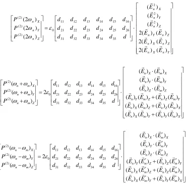
takes values from 1 to 6 according to Table 2.1. Using this conventional reduced notation, the nonlinear coefficient is a 3x6 matrix, which allows us to re-write equations (2-26) for second harmonic generation, sum and difference frequency mixing in three dimensions as follows:

⎥ ⎥ ⎥ ⎥ ⎥ ⎥ ⎥ ⎥ ⎦ ⎤ ⎢ ⎢ ⎢ ⎢ ⎢ ⎢ ⎢ ⎢ ⎣ ⎡ ⋅ ⎥ ⎥ ⎥ ⎦ ⎤ ⎢ ⎢ ⎢ ⎣ ⎡ = ⎥ ⎥ ⎥ ⎦ ⎤ ⎢ ⎢ ⎢ ⎣ ⎡ Y n X n Z n X n Z n Y n Z n Y n X n Z n Y n X n E E E E E E E E E d d d d d d d d d d d d d d d d d d P P P ) ( ) ( 2 ) ( ) ( 2 ) ( ) ( 2 ) ( ) ( ) ( ) 2 ( ) 2 ( ) 2 ( 2 2 2 35 34 33 32 31 26 25 24 23 22 21 16 15 14 13 12 11 0 ) 2 ( ) 2 ( ) 2 ( r r r r r r r r r ε ω ω ω ⎥ ⎥ ⎥ ⎥ ⎥ ⎥ ⎥ ⎥ ⎦ ⎤ ⎢ ⎢ ⎢ ⎢ ⎢ ⎢ ⎢ ⎢ ⎣ ⎡ + + + ⋅ ⋅ ⋅ ⋅ ⎥ ⎥ ⎥ ⎦ ⎤ ⎢ ⎢ ⎢ ⎣ ⎡ = ⎥ ⎥ ⎥ ⎦ ⎤ ⎢ ⎢ ⎢ ⎣ ⎡ + + + X m Y n Y m X n X m Z n Z m X n Y m Z n Z m Y n Z m Z n Y m Y n X m X n Z m n Y m n X m n E E E E E E E E E E E E E E E E E E d d d d d d d d d d d d d d d d d d P P P ) ( ) ( ) ( ) ( ) ( ) ( ) ( ) ( ) ( ) ( ) ( ) ( ) ( ) ( ) ( ) ( ) ( ) ( 2 ) ( ) ( ) ( 35 34 33 32 31 26 25 24 23 22 21 16 15 14 13 12 11 0 ) 2 ( ) 2 ( ) 2 ( r r r r r r r r r r r r r r r r r r ε ω ω ω ω ω ω ⎥ ⎥ ⎥ ⎥ ⎥ ⎥ ⎥ ⎥ ⎦ ⎤ ⎢ ⎢ ⎢ ⎢ ⎢ ⎢ ⎢ ⎢ ⎣ ⎡ + + + ⋅ ⋅ ⋅ ⋅ ⎥ ⎥ ⎥ ⎦ ⎤ ⎢ ⎢ ⎢ ⎣ ⎡ = ⎥ ⎥ ⎥ ⎦ ⎤ ⎢ ⎢ ⎢ ⎣ ⎡ − − − X m Y n Y m X n X m Z n Z m X n Y m Z n Z m Y n Z m Z n Y m Y n X m X n Z m n Y m n X m n E E E E E E E E E E E E E E E E E E d d d d d d d d d d d d d d d d d d P P P ) ( ) ( ) ( ) ( ) ( ) ( ) ( ) ( ) ( ) ( ) ( ) ( ) ( ) ( ) ( ) ( ) ( ) ( 2 ) ( ) ( ) ( * * * * * * * * * 35 34 33 32 31 26 25 24 23 22 21 16 15 14 13 12 11 0 ) 2 ( ) 2 ( ) 2 ( r r r r r r r r r r r r r r r r r r ε ω ω ω ω ω ω

where for space economy the argument of the electric fields (rr,t) has been neglected

and has been reduced to with similar argument

simplification for the sum and difference mixing components. ) , , 2 ( ) 2 ( n n n

P ω ω ω P(2)(2ω_n)

j,k X,X Y,Y Z,Z Y,Z Z,Y X,Z Z,X X,Y Y,X

l 1 2 3 4 5 6

It can be seen that an explicit use of Kleinman symmetry denotes that in the case of lossless crystals not all of the 18 elements of the nonlinear coefficient matrix are independent (for example, d₁₂ =d₁₂₂ =d₂₁₂ =d₂₆). Applying this idea systematically, the number of independent elements in the 3x6 coefficient matrix reduces to 10 and d

takes the form:

(2-45) ⎥ ⎥ ⎥ ⎦ ⎤ ⎢ ⎢ ⎢ ⎣ ⎡ = 14 13 23 33 24 15 12 14 24 23 22 16 16 15 14 13 12 11 d d d d d d d d d d d d d d d d d d d

Further reduction of the number of independent elements can be realised on the grounds of the crystal symmetry. For example, cubic crystals belonging to the 43m

class system (GaAs), present only three non vanishing elements and only one independent coefficient, resulting in the nonlinear coefficient matrix:

⎥ ⎥ ⎥ ⎦ ⎤ ⎢ ⎢ ⎢ ⎣ ⎡ = 14 14 14 0 0 0 0 0 0 0 0 0 0 0 0 0 0 0 d d d d

Establishing the exact expression for the nonlinear coefficient of a material allows the calculation of a scalar quantity which, for a specific wave interaction (i.e known propagation direction and polarisation axis of the waves), can be used with the scalar amplitudes of the interactive waves to describe the three wave mixing process. The calculation of this scalar effective nonlinear coefficient for the various crystal classes has been discussed in a number of sources [13-15] and allows the second harmonic generation, sum and difference frequency mixing to be expressed, respectively, via:

eff d | ) , ( | ) 2

( ₀ (2)

) 2 ( t r E d

P n eff n

r

ε

ω = (2-46 a)

| ) , ( || ) , ( | 2 ) ( ₀ ) 2 ( t r E t r E d

P ω_n +ω_m = _effε _n r _m r (2-46 b)

| ) , ( || ) , ( | 2 )

( ₀ *

) 2 ( t r E t r E d

P n m eff n m

r r

ε ω

ω − = (2-46 c) where is the scalar amplitude along the propagation direction of the wave at

| ) , ( |E_n rr t

n

2.3 Propagation of electromagnetic waves in nonlinear media

It has been shown that electromagnetic waves at given frequencies can induce a polarisation at other frequencies in appropriate (nonlinear) media. This induced polarisation will now be inserted as a source term in Maxwell equations (2-1) to unfold how this leads to the generation of new electromagnetic waves at the converted frequencies and how power is transferred between the interacting fields.

2.3.1 Coupled wave equations for nonlinear frequency conversion

Maxwell equations for a non-conductive, non-magnetic, source free second order nonlinear medium (i.e., Mr =Jr=ρ=0 and Pr(2) ≠0) are:

0 ) , ( ( ) ,

( ₀ =

∂ ∂ + ×

∇ H r t

t t r

Er r r r

r _µ (2-47 a) 0 ] ) , ( [ ) ,

( ₀ + (2) =

∂ ∂ − ×

∇ E r t P

t t r

Hr r r r r

r _{ε ε}

(2-47 b)

0 ) ,

( =

⋅

∇r Br rr t (2-47 c) 0

] )

, (

[ + (2) =

⋅

∇ o E r t P

r r r

r _{ε ε}

(2-47 d)

The trivial four-step process of formulating Maxwell equations in a wave motion equation [16] can be followed to obtain:

0 ) ) , ( ( ) , ( 2 ) 2 ( 2 2 2 0 0 2 = ∂ ∂ + ∂ ∂ − ∇ t P t t r E t r E _r r r r r r ε ε

µ (2-48)

In the absence of the nonlinear source term, Eq. (2-48) decays to the standard linear wave equation. Without compromising the physical context of the nonlinear wave equation, the treatment can be simplified by considering fields propagating in the z -axis. Eq. (2-48) can then be written in a scalar form:

( , ) ( ( , ) ) 0

2 ) 2 ( 2 2 2 0 0 2 2 = ∂ ∂ + ∂ ∂ − ∂ ∂ t P t t z E z t z

Er r r

ε ε

µ (2-49)

Assuming that the nonlinear term is “small” compared to the linear one, plane-wave-like solutions can be adopted, with the proper introduction of a complex field amplitudeEr(z), which is not a constant as in Eq. (2-13), but a slowly varying function of z:

] . ) ( ) ( ) ( [ 2 1 ) ,

(_{z t E z e}( 1 1) _{E z e}( 2 2) _{E z e} ( 3 3) _cc

Each individual frequency component of the field is required to satisfy Eq. (2-49). Taking as an example the sum frequency component ω3= ω1+ω2 and substituting the nonlinear polarisation term by use of Eq. (2-46 b), the wave equation gives:

− ∂ ∂ − ∂ ∂ − − ] [ ) ( ) ( ( ) 2 2 3 0 0 ) ( 3 2 2 3 3 3

3z t ikz t

k i e t z E e z E z ω

ω _{µ ε ε}

0 ]} [ ) ( ) (

2 [( ) ( )]

2 2 2 1 0 0 2 1 2 1 = ∂ ∂

− i k+k z− + t

eff e t z E z E

d ω ω

ε µ

Carrying out the calculations for the derivatives and ignoring the term , which is an acceptable approximation within the limits of the slowing varying envelope assumption, we find:

2 3

2

/ ) (z dz E d 0 ) ( ) ( 2 ) ( ) ( ) (

2 1 2 ( )

2 3 0 0 3 2 3 0 3 2 3 3 3 3 2 1 = + +

− ik+k −k z

eff r

o E z d E z E z e

z E k dz z dE

ik µ ε ε ω µ ε ω

Similar expressions can be found for the waves at ω2=ω3-ω1 and ω1=ω3-ω2, substituting this time the nonlinear term with the difference frequency polarisation component given by (2-46 c). With appropriate use of equations (2-8), (2-14) and introducing the definition:

1 2

3 k k

k

k= − −

∆ (2-51) these expressions can be rewritten in the most commonly used form:

kz i effE z E z e

d c n i dz z dE _∆ = ( ) ( ) ) ( * 2 3 1 1 1 ω (2-52 a) kz i effE z E z e

d c n i dz z dE _∆ = ( ) ( ) ) ( * 1 3 2 2 2 ω (2-52 b) kz i effE z E z e

d c n i dz z

dE _−∆

= ( ) ( ) ) ( 2 1 3 3 3 ω (2-52 c)

Equations (2-58) are called “coupled wave equations” and describe the general three wave mixing process. They manifest that the interacting fields are coupled through the nonlinear coefficient, , which enables energy flow from one frequency component to another.

eff

Similarly, the driving polarisation component at the second harmonic (2-46 a) can be used to obtain the following set of coupled wave equations for second harmonic generation:

kz i effE z E z e

d c n i dz z dE _∆ = ( ) ( ) ) ( *

2ω ω

ω

ω ω

(2-53 a)

kz i effE z e

d c n i dz z

dE _−∆

= ( ) 2 2 ) ( 2 2 2 ω ω ω ω (2-53 b)

2.3.2 The Manley-Rowe relations

The coupled wave equations can be rewritten in an equivalent form by substituting the electric fields with the intensity of the electromagnetic wave, which is defined through: ) ( ) ( ) ( 2

1 1/2 *

0 0 z E z E n

I_{i i i i}

µ ε

= (2-54)

The spatial variation of the intensity corresponding to the frequency component ω1 (for example) is then:

)] ( ) ( ) ( ) ( [ ) ( 2 1 1 * 1 * 1 1 1 2 / 1 0 0 1 z E dz d z E z E dz d z E n dz dI + = µ ε

Inserting (2-52 a), the last equation gives:

⇔ + − = −∆ ∆ ] ) ( ) ( ) ( ) ( ) ( ) )( ( [ ) ( 2 1 * 2 3 * 1 2 * 3 1 1 1 1 2 / 1 0 0

1 i kz i kz

eff E z i E z E z e iE z E z E z e

d c n n dz dI ω µ ε ] } ) ( ) ( ) ( { } ) ( ) ( ) ( { [ ) ( 2 1 * 3 * 2 * 1 3 * 2 * 1 1 1 1 2 / 1 0 0

1 i kz i kz

eff i E z E z E z e i E z E z E z e

d c n n dz

dI _{∆ ∆}

−

= ω

µ ε

Similar expressions can be found for the other two frequency components. Using the

identity: and after some rearrangement, these

expressions can be written in the form: ) Im( ) Im( ) ( 2 /

1 iA−iA* =− A = A*

} ) ( ) ( ) (

Im{ ₁* ₂* ₃

1 2 0

1 i kz

eff E z E z E z e

d c dz

dI _∆

−

= ε ω (2-55 a)

} ) ( ) ( ) ( Im{ 3 * 2 * 1 2 2 0

2 i kz

eff E z E z E z e

d c dz

dI ₌₋ε _ω ∆

(2-55 b) } ) ( ) ( ) ( Im{ 3 * 2 * 1 3 2 0

3 i kz

eff E z E z E z e

d c dz

dI _∆

=ε ω (2-55 c)

) ( )

( ) (

3 3 2

2 1

1

ω ω

ω

I dz

d I

dz d I dz

d

− =

= (2-56)

Relations (2-55), known as Manley-Rowe relations, describe the intensity change for the three interacting waves. They clearly imply that the growth of one field component will be at the expense of another of the fields coupled through the nonlinear coefficient. In an equivalent frame, they manifest the conservation of the total intensity field. This can also be viewed mathematically through the following equation, which is always satisfied due to Eqs. (2-55):

0

3 2

1 + + =

dz dI dz dI dz dI

(2-57)

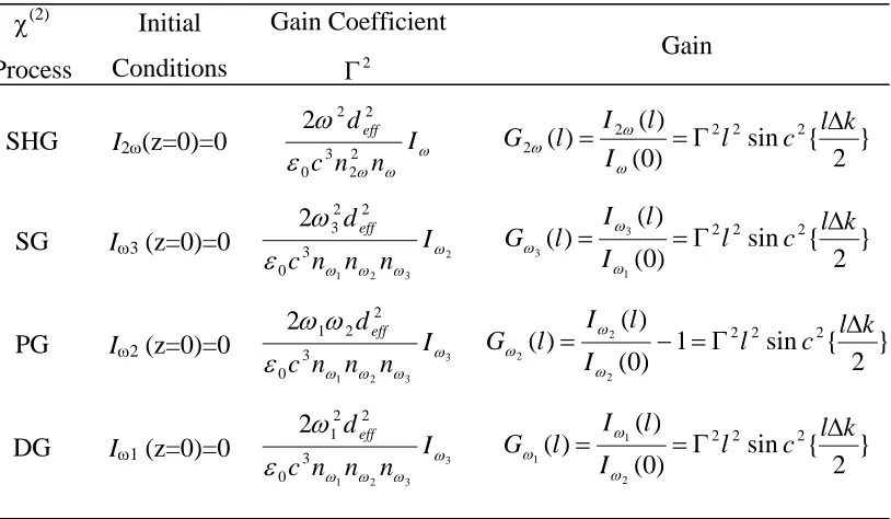
2.3.3 Second order nonlinear frequency conversion processes and gain

Having established the coupled differential equations (2-52) and (2-53) that govern the interaction of three waves in a nonlinear medium, it is evident that four distinctive processes are possible, shown schematically in Fig. 2.1. These processes, namely second harmonig generation (SHG), sum generation (SG), parametric generation (PG) and difference generation (DG), are identical in their nature but differ in the direction of power growth.

Power growth

Power decay

Second harmonic generation

Parametric generation

Sum generation Difference generation

ω ω 2ω

ω1

ω2

ω3

ω1

ω2

ω3

ω1

ω2

ω3

Power growth

Power decay

Second harmonic generation

Parametric generation

Sum generation Difference generation

ω ω 2ω

ω1

ω2

ω3

ω1

ω2

ω3

ω1

ω2

ω3

Calculating the gain of a specific interaction requires solving the coupled wave equations. The general treatment of this problem can be found in [1]. For the scope of the present discussion, an example will be given through the special case of the undepleted second harmonic generation.

The coupled wave equations for second harmonic generation (2-53), assuming that the driving field at ω does not undergo strong depletion, and hence , give:

const E

z

E_ω( )= _ω =

⇒ =

∫

∫

( i kl

kl i kl i eff e k l i e e E ld c n i E l

E −∆

∆ − ∆ ∆ − = − _ω ω ω ω ω

where l is the interaction length. Assuming the initial condition of zero input second harmonic field, the last equation takes the form:

2 / 2 2 2 } 2 { sin )

( ld_effE c l k e i kl c

n i l

E = _ω ∆ −∆

ω ω

ω

(2-58)

where by definition: . Multiplying the last equation with its complex conjugate, a similar expression can be obtained in terms of the field intensities: ) 2 /( ) ( / sin ) (

sincx = x x= eix−e−ix ix

⇒ ∆ = } 2 { sin ] [ ) ( ) ( )

( 2 * 2 2

2 * 2 2 k l c E E ld c n l E l

E eff ω ω

ω ω ω ω ⇒ ∆ = − } 2 { sin ] ) ( 2 1 [ ) ( )

( 1/2 1 2

0 0 2 2 2 2 k l c n I ld c n l

I eff ω ω

ω ω _µ ε ω } 2 { sin ] 2 [ )

( 2 2

2 2 2 3 0 2 2 2 k l c I n n n c d l l

I = eff ⋅ _ω ⋅ ∆

ω ω ω ω

ω

ε (2-59) The intensity gain experienced by the second harmonic field is thus:

} 2 { sin ) ( )

( 2 2 2 2

2 k l c l I l I l

G = =Γ ∆

ω ω

ω (2-60)

where the gain coefficient Γ has been introduced, such as:

ω ω ω ε ω I n n c deff 2 2 3 0 2 2 2 = 2