C
2013. The American Astronomical Society. All rights reserved. Printed in the U.S.A.
THE CLUSTERING OF GALAXIES IN THE SDSS-III BARYON OSCILLATION SPECTROSCOPIC SURVEY:
LUMINOSITY AND COLOR DEPENDENCE AND REDSHIFT EVOLUTION
Hong Guo1,2, Idit Zehavi1, Zheng Zheng2, David H. Weinberg3, Andreas A. Berlind4, Michael Blanton5, Yanmei Chen6, Daniel J. Eisenstein7, Shirley Ho8,9, Eyal Kazin10, Marc Manera11, Claudia Maraston11,12,
Cameron K. McBride7, Sebasti ´an E. Nuza13, Nikhil Padmanabhan14, John K. Parejko14, Will J. Percival11, Ashley J. Ross11, Nicholas P. Ross8, Lado Samushia11,15, Ariel G. S ´anchez16, David J. Schlegel8,
Donald P. Schneider17,18, Ramin A. Skibba19, Molly E. C. Swanson7, Jeremy L. Tinker5, Rita Tojeiro11,
David A. Wake20,21, Martin White8,22,23, Neta A. Bahcall24, Dmitry Bizyaev25, Howard Brewington25, Kevin Bundy26,
Luiz N. A. da Costa27,28, Garrett Ebelke25, Elena Malanushenko25, Viktor Malanushenko25, Daniel Oravetz25,
Graziano Rossi29,30, Audrey Simmons25, Stephanie Snedden25, Alina Streblyanska31,32, and Daniel Thomas11,12
1Department of Astronomy, Case Western Reserve University, OH 44106, USA 2Department of Physics and Astronomy, University of Utah, UT 84112, USA 3Department of Astronomy and CCAPP, Ohio State University, Columbus, OH 43210, USA
4Department of Physics and Astronomy, Vanderbilt University, Nashville, TN 37235, USA 5Center for Cosmology and Particle Physics, New York University, New York, NY 10003, USA
6Department of Astronomy, Nanjing University, Nanjing 210093, China 7Harvard-Smithsonian Center for Astrophysics, 60 Garden St., Cambridge, MA 02138, USA
8Lawrence Berkeley National Laboratory, 1 Cyclotron Road, Berkeley, CA 94720, USA 9Department of Physics, Carnegie Mellon University, 5000 Forbes Avenue, Pittsburgh, PA 15213, USA
10Center for Astrophysics and Supercomputing, Swinburne University of Technology, P.O. Box 218, Hawthorn, Victoria 3122, Australia 11Institute of Cosmology & Gravitation, Dennis Sciama Building, University of Portsmouth, Portsmouth, PO1 3FX, UK
12SEPnet, South East Physics Network,www.sepnet.ac.uk
13Leibniz-Institut f¨ur Astrophysik Potsdam (AIP), An der Sternwarte 16, D-14482 Potsdam, Germany 14Department of Physics, Yale University, 260 Whitney Ave, New Haven, CT 06520, USA
15National Abastumani Astrophysical Observatory, Ilia State University, 2A Kazbegi Ave., GE-1060 Tbilisi, Georgia 16Max-Planck-Institut f¨ur extraterrestrische Physik, Postfach 1312, Giessenbachstr., D-85748 Garching, Germany 17Department of Astronomy and Astrophysics, The Pennsylvania State University, University Park, PA 16802, USA
18Institute for Gravitation and the Cosmos, The Pennsylvania State University, University Park, PA 16802, USA 19Center for Astrophysics and Space Sciences, University of California, 9500 Gilman Drive, San Diego, CA 92093, USA
20Department of Astronomy, Yale University, New Haven, CT 06520, USA
21Department of Astronomy, University of Wisconsin-Madison, 475 N. Charter Street, Madison, WI 53706, USA 22Department of Physics, University of California, 366 LeConte Hall, Berkeley, CA 94720, USA 23Department of Astronomy, 601 Campbell Hall, University of California at Berkeley, Berkeley, CA 94720, USA
24Princeton University Observatory, Princeton, NJ 08544, USA 25Apache Point Observatory, P.O. Box 59, Sunspot, NM 88349-0059, USA
26Kavli Institute for the Physics and Mathematics of the Universe, University of Tokyo, Kashiwa 277-8582, Japan 27Observat´orio Nacional, Rua Gal. Jos´e Cristino 77, Rio de Janeiro, RJ - 20921-400, Brazil
28Laborat´orio Interinstitucional de e-Astronomia - LineA, Rua Gal. Jos´e Cristino 77, Rio de Janeiro, RJ - 20921-400, Brazil 29CEA, Centre de Saclay, Irfu/SPP, F-91191 Gif-sur-Yvette, France
30Paris Center for Cosmological Physics (PCCP) and Laboratoire APC, Universit´e Paris 7, F-75205 Paris, France 31Instituto de Astrofisica de Canarias (IAC), E-38200 La Laguna, Tenerife, Spain
32Dept. Astrofisica, Universidad de La Laguna (ULL), E-38206 La Laguna, Tenerife, Spain
Received 2012 December 5; accepted 2013 March 7; published 2013 April 4
ABSTRACT
We measure the luminosity and color dependence and the redshift evolution of galaxy clustering in the Sloan Digital Sky Survey-III Baryon Oscillation Spectroscopic Survey Ninth Data Release. We focus on the projected two-point correlation function (2PCF) of subsets of its CMASS sample, which includes about 260,000 galaxies over∼3300 deg2 in the redshift range 0.43< z <0.7. To minimize the selection effect on galaxy clustering, we construct well-defined luminosity and color subsamples by carefully accounting for the CMASS galaxy selection cuts. The 2PCF of the whole CMASS sample, if approximated by a power-law, has a correlation length of
r0 = 7.93±0.06h−1Mpc and an index of γ = 1.85±0.01. Clear dependences on galaxy luminosity and color are found for the projected 2PCF in all redshift bins, with more luminous and redder galaxies generally exhibiting stronger clustering and steeper 2PCF. The color dependence is also clearly seen for galaxies within the red sequence, consistent with the behavior of SDSS-II main sample galaxies at lower redshifts. At a given luminosity (k+e corrected), no significant evolution of the projected 2PCFs with redshift is detected for red sequence galaxies. We also construct galaxy samples of fixed number density at different redshifts, using redshift-dependent magnitude thresholds. The clustering of these galaxies in the CMASS redshift range is found to be consistent with that predicted by passive evolution. Our measurements of the luminosity and color dependence and redshift evolution of galaxy clustering will allow for detailed modeling of the relation between galaxies and dark matter halos and new constraints on galaxy formation and evolution.
Key words: cosmology: observations – cosmology: theory – galaxies: distances and redshifts – galaxies: halos – galaxies: statistics – large-scale structure of universe
1. INTRODUCTION
Galaxies in the universe are observed to display a wide range of properties, such as luminosity, color, stellar mass, age, morphology, and spectral type. These properties encode information about galaxy formation and evolution and are related to the environment hosting the galaxies. Different populations of galaxies are thus expected to trace the underlying dark matter distribution in different ways.
Contemporary galaxy redshift surveys, most notably the Sloan Digital Sky Survey (SDSS; York et al.2000), have trans-formed the study of large-scale structure, enabling pristine mea-surements and detailed studies of galaxy clustering. Galaxy clustering provides a powerful approach to probe the complex relation between galaxies and the underlying dark matter distri-bution (e.g., Kaiser1984). The dependence of galaxy clustering on galaxy properties has been observed in numerous galaxy sur-veys (e.g., Davis & Geller1976; Davis et al. 1988; Hamilton 1988; Loveday et al.1995; Benoist et al. 1996; Guzzo et al. 1997; Norberg et al.2001, 2002; Zehavi et al. 2002,2005b, 2011; Budav´ari et al. 2003; Madgwick et al.2003; Li et al. 2006; Coil et al.2006,2008; Meneux et al.2006,2008,2009; Wang et al.2007; Wake et al.2008,2011; Swanson et al.2008; Ross & Brunner2009; Skibba et al.2009; Loh et al.2010; Ross et al. 2010, 2011b; Christodoulou et al. 2012; Mostek et al. 2012).
In general, more luminous and redder galaxies are found to be more strongly clustered than their fainter and bluer counter-parts. Similarly, early-type (elliptical) galaxies exhibit stronger clustering than late-type (spiral) ones. Galaxy luminosity and color are perhaps the two major readily observed properties, which also facilitate comparison between different surveys and are less dependent on the stellar evolution models. Moreover, they have proven to be the two properties most predictive of galaxy environment, such that any residual dependence on mor-phology or surface brightness is weak (Blanton et al. 2005). In this paper, we measure the dependence of galaxy cluster-ing on color and luminosity for galaxies in the SDSS-III Baryon Oscillation Spectroscopic Survey (BOSS; Eisenstein et al.2011; Dawson et al.2013) and study the implications.
Galaxy clustering measurements, once properly interpreted, can provide key information about galaxy formation and evo-lution. In particular, the theoretical understanding of galaxy clustering has been greatly advanced with the development of dark matter halo models (see Cooray & Sheth2002and refer-ences therein). In the cosmological constant + cold dark matter (ΛCDM) paradigm, galaxies form and evolve in dark matter ha-los. While the properties and clustering of dark matter halos are well understood with the help of analytic models and numerical simulations (e.g., Mo & White1996; Springel et al.2005), the properties of galaxies are hard to predict because of the complex baryonic processes and the lack of complete theory of galaxy formation.
Galaxy clustering offers an opportunity to connect galaxies to dark matter halos, providing a new direction in studying galaxy formation and evolution. The halo occupation distri-bution (HOD) framework (see, e.g., Peacock & Smith2000; Seljak 2000; Scoccimarro et al. 2001; Berlind & Weinberg 2002; Berlind et al.2003; Zheng et al. 2005) or the closely related conditional luminosity function (CLF) method (Yang et al.2003,2005) describe the number of galaxies as a function of halo mass, and galaxy clustering is used to constrain the HOD or CLF parameters. The subhalo abundance matching method
makes use of subhalos in high resolution N-body simulations and connects them to galaxies to interpret galaxy clustering (see, e.g., Kravtsov et al.2004; Conroy et al.2006; Guo et al. 2010; Nuza et al.2012). Such models essentially convert galaxy clustering measurements to the relation between galaxies and halos, which provides strong tests of galaxy formation models. The galaxy-halo connections inferred at different redshifts, together with the theoretically known halo evolution, can lead to empirical constraints on galaxy evolution. For example, Zheng et al. (2007) compare the HODs forz∼1 DEEP2 andz∼0 SDSS galaxies and find a halo mass dependent growth of stellar mass of central galaxies, separating into contributions from star formation and mergers. Tinker & Wetzel (2010) analyze four samples of galaxies from redshiftz = 0.4 toz = 2.0. They find that more than 75% of the red satellite galaxies move onto the red sequence because of halo mergers, while the mechanism for central galaxies to move to the red sequence evolves from
z=0.5 toz=0.
To advance our understanding of galaxy evolution, improved measurements of galaxy clustering in large galaxy surveys at different redshifts are necessary. The color and luminosity dependence of clustering has been studied in detail at z ∼ 1 for DEEP2 galaxies (Coil et al. 2008) and at z ∼ 0 for SDSS galaxies (Zehavi et al.2011; denoted Z11 hereafter). The trends with color and luminosity are generally similar. However, while Coil et al. (2008) find no changes of the clustering within the red sequence,Z11find a continuous trend (in both amplitude and slope) of stronger clustering with color in SDSS galaxies. This discrepancy may be caused by different sample selections, but it may also be a signature of galaxy evolution (e.g., related to the buildup of red sequence). Studying a sample from an intermediate redshift range can provide new important information and a better understanding of galaxy evolution.
In this paper, we use the recently released CMASS sample of the BOSS Data Release 9 (DR9; Ahn et al.2012) to measure the clustering of galaxies in the redshift range 0.43< z <0.7 and study the dependence on galaxy luminosity and color. The sample is constructed to contain a roughly volume-limited set of massive and luminous galaxies (with a typical stellar mass of 1011.3h−1M
; Maraston et al.2012) in this redshift range. This sample has recently been used to accurately measure the baryon acoustic oscillation (BAO) signature (see Weinberg et al.2012for a recent comprehensive review) on large scales (∼100h−1Mpc) by Anderson et al. (2012). The sample has been thoroughly vetted, and the robustness of the results and cosmological constraints from the BAO and redshift-space distortions are explored in a series of papers (Reid et al.2012; Ross et al.2012,2013; S´anchez et al.2012; Samushia et al.2013; Sc´occola et al.2012; Tojeiro et al.2012a,2012b). The smaller scale clustering measurements and HOD fits are first presented by White et al. (2011) (for an earlier smaller sample) and Nuza et al. (2012). Here we study the small to intermediate scale (0.05–25h−1Mpc) two-point correlation functions (2PCFs) of CMASS galaxies, focusing especially on the dependence on luminosity and color and the implications on galaxy evolution from simple models. We will study the evolution of CMASS galaxies based on HOD modeling in a companion paper.
Section4. AppendixAdiscusses the effect of different stellar evolution models on our results, and AppendixBexplores the robustness of the jackknife error estimates used.
Throughout the paper, we assume a spatially flat ΛCDM cosmology as in Anderson et al. (2012), with Ωm = 0.274,
h = 0.7, Ωbh2 = 0.0224, ns = 0.95, and σ8 = 0.8, consistent with the best-fit model from theWilkinson Microwave Anisotropy Probe7-year data (Komatsu et al.2011).
2. OBSERVATIONS AND METHODS
2.1. Data
As part of the SDSS-III survey, BOSS selects luminous galaxies from the multiple-band SDSS imaging (Fukugita et al. 1996; Gunn et al.1998,2006; York et al.2000) for spectroscopic observation to probe the large-scale BAO signals (Anderson et al. 2012). Dawson et al. (2013) provide a comprehensive overview of BOSS, while the technical details of BOSS are presented in Smee et al. (2012) and Bolton et al. (2012). The selection of BOSS galaxies is a union of targets in two different redshift intervals. One is an extension of the SDSS-I/II Luminous Red Galaxy (LRG) sample (Eisenstein et al.2001), referred to as LOWZ with 0.2< z <0.43 (Parejko et al.2013). The other, denoted as CMASS (White et al.2011; Anderson et al. 2012), includes ∼260,000 galaxies in DR9, and is approximately stellar-mass limited at higher redshifts (0.43< z <0.7) with an effective volume of∼2.2 Gpc3and an effective area of about 3300 deg2. In this paper, our study focuses on the CMASS sample. The target selection cuts for CMASS galaxies are fainter and bluer than the LRG sample in order to achieve a higher number density of about 3×10⁻⁴h3Mpc−3and sample a wider range of galaxies. The detailed target selection of the CMASS sample is described in N. Padmanabhan et al. (2013, in preparation), and summarized in Eisenstein et al. (2011) and Anderson et al. (2012). We briefly describe here the major selection cuts that will affect our analysis of luminosity and color dependence of the 2PCF.
The CMASS sample aims at selecting galaxies following a roughly constant stellar mass cut at redshiftz > 0.4. The selection criteria of the CMASS galaxies are defined by,
17.5< icmod<19.9 (1)
d⊥>0.55, (2)
icmod<19.86 + 1.6(d⊥−0.8) (3)
ifib2<21.5 (4)
rmod−imod<2.0 (5)
whered⊥is defined as
d⊥=rmod−imod−(gmod−rmod)/8 (6)
and all magnitudes are extinction corrected (Schlegel et al. 1998) and are in the observed frame. While the magnitudes are calculated usingcmodelmagnitudes (denoted by the subscript “cmod”), the colors are computed using model magnitudes (denoted by the subscript “mod”; see Anderson et al. 2012 for details). The magnitudeifib2corresponds to thei-band flux within the 2fiber size. CMASS objects also pass specific star-galaxy separation cuts, as described in Anderson et al. (2012).
2.2. Selection Cuts and Sample Completeness
The CMASS galaxies are chosen by applying complex target selection cuts, and it is thus difficult to construct exact volume-limited samples. Since we intend to investigate the luminosity and color dependence of galaxy clustering in this paper, we must pay particular attention to the completeness in luminosity and color. With this goal in mind, we first investigate the target selection cuts projected to the color–luminosity plane at different redshifts, which will provide the appropriate boundaries in constructing our samples.
Figure1shows the color–magnitude diagram (CMD) at six narrow redshift ranges withΔz=0.05. The contours represent the number density distribution of CMASS galaxies in the CMD. The absolute magnitudeMiandr−icolor arek+ecorrected to
z =0.55 throughout the paper using a global Flexible Stellar Population Synthesis (FSPS) model (Conroy et al.2009; Conroy & Gunn2010; Tojeiro et al.2011,2012b). Using other stellar evolution models slightly changes the resulting magnitudes and colors, but does not affect our analysis of galaxy clustering, as we discuss in AppendixA. In each panel of Figure1, only the approximate positions of the selection cuts are shown as dashed lines, since the selection cuts are made in apparent magnitudes and in three bands (g, r,and,i) while our CMD is shown forr−i color andMimagnitude. The slopes of the dashed lines follow the boundaries seen in the CMD contours in each redshift bin. We focus on the three main cuts (Equations (1)–(3)). Following Zehavi et al. (2011), we adopt a luminosity-dependent color cut to separate red and blue galaxies (discussed in detail in Section3.3),
(r−i)cut=0.679−0.082(Mi+ 20), (7)
represented by the green lines in Figure1.
The horizontal cut in each panel corresponds to the i-band faint-end flux limit (Equation (1), i < 19.9), which selects galaxies brighter than the corresponding absolute magnitude at each redshift. The slightly tilted vertical dashed line on the left of the distribution is thed⊥ cut (Equation (2)), which removes galaxies with bluer colors and with lower redshifts (Cannon et al.2006; N. Padmanabhan et al. 2013, in preparation). The bottom-left dashed line is thei-band sliding cut (Equation (3)), which excludes the fainter and bluer (thus lower stellar mass) galaxies from the sample. These three main cuts evolve with redshift. A consequence of the d⊥ and sliding cuts is that there are more blue galaxies at higher redshifts. Atz >0.55, while the CMASS sample is less affected by the d⊥ cut, the sliding cut must be carefully taken into account at all redshifts in constructing complete galaxy samples. At z < 0.55, blue galaxies are highly incomplete (see an estimation of the fraction of star-forming galaxies in CMASS in Figure 16 of Chen et al. 2012). Atz <0.45, thed⊥cut leads to incompleteness even for the most luminous red galaxies.
Figure 1.Color–magnitude diagram (CMD) of CMASS galaxies in different redshift intervals. Both magnitude and color arek+ecorrected toz=0.55. The contours represent the number density distribution of CMASS galaxies in the CMD. The approximate positions of the selection cuts are shown as dashed lines in each panel, labeled with the corresponding equation numbers of the selection cuts (see the text). The green solid lines are our color cut (Equation (7)) for red and blue galaxies. (A color version of this figure is available in the online journal.)
approximately complete galaxy samples. As we proceed in our analysis, we keep in mind the boundaries of “completeness” defined by the selection cuts when constructing our galaxy sam-ples. One advantage of such an empirical method is that it is largely model-independent.
2.3. Clustering Measurements
In this paper, we focus our discussion on the galaxy 2PCF. We use the Landy–Szalay estimator (Landy & Szalay1993) to measure the 2PCF of galaxies,
ξ(r)= DD−2DR + RR
RR (8)
where DD, DR and RR are the data–data, data–random, and random–random pair counts measured from the data of N galaxies and random samples consisting ofNR random points. These pair counts are appropriately normalized byN(N−1)/2, NNR, andNR(NR−1)/2, respectively.
We measure the three-dimensional (3D) 2PCF ξ(rp, rπ), whererpandrπare the separations of galaxy pairs perpendicular and parallel to the line of sight. The redshift-space 2PCF
ξ(rp, rπ) differs from the real-space one because of redshift distortions induced by galaxy peculiar velocities. The redshift distortions can be mitigated by projecting the 2PCF along the line-of-sight direction, with the projected 2PCFwp(rp) (Davis & Peebles1983) defined and measured as
wp(rp)=2
∞
0
ξ(rp, rπ)drπ =2
i
ξ(rp, rπ,i)Δrπ,i (9)
whererπ,iandΔrπ,iare theith bin of the line-of-sight separation and its corresponding bin size. In practice, we sum ξ(rp, rπ) along the line-of-sight direction up torπ,max =80h−1Mpc to include most of the correlated pairs. As our analysis focuses
on 2PCF measurements up torp ∼25h−1Mpc, the clustering measurements do not depend significantly on the assumedrπ,max once it is sufficiently larger. For example, if we integrate the line-of-sight direction to 200h−1Mpc, the contribution from 80h−1Mpc < r
π < 200h−1Mpc to wp(rp) only introduces noisy fluctuations of about 2%.
The projected 2PCF can be related to the real-space correla-tion funccorrela-tion,ξ(r), by
wp(rp)=2
∞
rp
r dr ξ(r)r2−rp2−1/2 (10)
(Davis & Peebles1983). It is common practice to characterize
ξ(r) by a power law on small scales,ξ(r) =(r/r0)−γ, and in such a casewp(rp) can be expressed as
wp(rp)=rp
r0
rp γ
Γ
1 2
Γ
γ −1
2 Γ
γ
2
. (11)
The covariance matrix of the correlation function is estimated using the jackknife resampling method (following Zehavi et al. 2005b,2011)
Cov(ξi, ξj)=
N−1
N
N
l=1
ξil− ¯ξi
ξjl− ¯ξj
(12)
where N ≡ 100 is the total number of jackknife samples, ξil
We focus on analyzing our measurement of the galaxy 2PCF on the small to intermediate scales (0.05h−1Mpc < r
p < 25h−1Mpc), aiming at probing the relation between galaxies and their host halos. However, the small-scale measurement of the 2PCF is limited by the fiber collision effect in the spectrograph system of SDSS-III, where two fibers on the same plate cannot be placed closer than an angular separation of 62 (Dawson et al. 2013; Anderson et al. 2012). As a result, about 5.5% of CMASS galaxies do not have redshifts, strongly affecting small-scale clustering measurements. We correct for this effect using the method proposed and tested by Guo et al. (2012), which divides the galaxy sample into two distinct populations, one free of fiber collisions (referred to as D1) and the other consisting of potentially collided galaxies (denoted as D2). The total clustering signal is a combination of the contributions from these two populations, where the contribution of the collided population is estimated from the resolved galaxies in tile-overlap regions.
As discussed in detail in Guo et al. (2012), there are two main systematics that could impact the accuracy of such a method to treat fiber collisions. One is possible density variations between the tile overlap and non-overlap regions, which is found to be insignificant from tests with mock galaxy catalogs. Another effect is that galaxies in collided triplets (or even higher-order colliding groups) can only be fully recovered in regions covered by at least three tiles, making the estimation from close pairs in two-tile regions not accurate (because of the lack of D2D2close pairs). This effect is alleviated by an additional correction term using the measured close pairs in the two-tile regions. After full application of the Guo et al. (2012) method, we estimate the remaining systematic errors to be less than 3%–5%. It is generally difficult to have an unbiased correction on all scales, but this approach provides the best estimate of the galaxy 2PCF on small scales, compared with other possible methods.
When counting pairs for the 2PCF, each galaxy is assigned a series of weights to reduce variance in the measurements and take into account different effects. Following Anderson et al. (2012), we apply a scale-independent weight to optimize the clustering measurements (Feldman et al.1994)
wFKP= 1 1 +n¯(z)P0
, (13)
where n¯(z) is the mean density at redshift z, and P0 = 2×10⁴h−3Mpc3. This equation provides similar results to the minimum variance weight used by Hamilton (1993) and Zehavi et al. (2002). Another employed weight,wrf, accounts for the fact that not every galaxy with a spectrum taken has a reliable redshift measurement. The “redshift failures” are dependent on the positions of fibers on the plates (Ross et al. 2012) and are corrected by up-weighting the nearest galaxy that has an accurate redshift. The final weight,wsys, is caused by the scarcity of galaxies detected due to foreground bright stars (Ross et al.2011a). Ross et al. (2012) present a comprehensive study of potential systematic effects in the 2PCF analysis, and compute a set of weightswsysbased on the stellar density andifib2
magnitude. Therefore, the total weight applied to each galaxy is
wtot=wFKPwsyswrf. (14)
The quantitywtotis applied to both the D1and D2 populations in the fiber collision correction. The systematic weight wsys
only has a small effect on small and intermediate scales, but significantly changes the clustering measurements on BAO scales.
We construct the random catalogs according to the detailed angular selection of the DR9 galaxy sample. The radial selection function for each sample is taken into account by assigning the shuffled galaxy redshifts to the random objects. The shuffling method provides a better representation of the true distribution compared with a smooth spline fit to the observed galaxy redshift distribution, as detailed in Ross et al. (2012). This process is done separately for the northern and southern Galactic Caps to account for the different number density distributions (see Anderson et al. 2012 for details). To apply the fiber collision correction, separate random catalogs for the D1 and D2populations are used. Denoting the fraction of recovered D2 galaxies as N2/N2, for the D2 random catalogs we apply an additional angular maskN2/N2 in each sector (see Guo et al.
2012for details).
3. RESULTS
3.1. 2PCF of the Full CMASS Sample
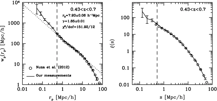
Before presenting the luminosity and color dependence of the 2PCFs for CMASS galaxies, we show in Figure 2 the projected and redshift-space 2PCFs for the entire CMASS sample in the redshift range 0.43 < z < 0.7 (solid lines). For comparison, we also display the recent CMASS DR9 measurements of Nuza et al. (2012, open symbols), which are limited to slightly larger scales (0.5h−1Mpc) and show good agreement on all measured scales. The vertical dashed lines indicate the maximal fiber collision scale, ∼0.53h−1Mpc at redshift z = 0.7. By applying the fiber-collision correction method of Guo et al. (2012), we are able to robustly measure the small-scale clustering (note the small error bars). This should enable better constraints on the spatial distribution of galaxies inside dark matter halos and a better constraint on the fraction of satellite galaxies, which we will address in future work.
The dotted line in the left panel of Figure2 is the power-law fit towp for 0.05h−1Mpc < rp <25h−1Mpc, based on Equation (11), using the full error covariance matrix. Although
wp clearly deviates from a power-law (also shown from the
χ2/dof of the fitting), a power-law fit provides a simple char-acterization of the clustering and allows for easy comparisons among the 2PCFs of different galaxy samples. The correlation length for the CMASS sample isr0=7.93±0.06h−1Mpc and the slopeγ =1.85±0.01 (note that given the large bestfitχ2, the error bars here should be interpreted with care). These val-ues are similar to clustering measurements of LRGs atz∼0.55 from the 2dF-SDSS LRG and QSO (2SLAQ) survey (Cannon et al. 2006; Ross et al.2007; Wake et al.2008), as expected, since the CMASS galaxy color selections were based on the 2SLAQ LRG selection.
Figure 2.Projected (left panel) and redshift-space(right panel) 2PCFs for the entire CMASS sample in the range of 0.43< z <0.7. The solid lines present our measurements. The open symbols are the recent measurements of Nuza et al. (2012), which are in good agreement. The vertical dashed lines correspond to the maximal fiber collision scale (∼0.53h−1Mpc) forz=0.7. The dotted line in the left panel is a power-law fit tow
pfor 0.05h−1Mpc< rp<25h−1Mpc with the
corresponding parameters as labeled.
Figure 3.Color–magnitude diagrams of CMASS galaxies in the two redshift bins we use, as well as overall distribution of galaxies ini-band absolute magnitude and redshift. The red lines delineate the luminosity bin samples we study. The two green lines in the right panel represent thei-band flux limits of Equation (1), which is alsok+ecorrected toz=0.55.
(A color version of this figure is available in the online journal.)
the redshift-space 2PCFξ(s) on scales aboves >0.1h−1Mpc, where it can be reliably measured. The fiber collisions in that case impact larger scales than indicated by the dashed line, since sincludes the contribution from the line-of-sight separations,
s2=r2
p+rπ2(see more discussion in Guo et al.2012).
3.2. Luminosity Dependence
3.2.1. Luminosity Cuts
We now investigate the luminosity dependence of CMASS galaxy clustering. To minimize the influence of sample incom-pleteness, we carefully construct samples of different luminosi-ties by accounting for the selection cuts as a function of red-shifts discussed in Section 2.2. We divide galaxies into two redshift bins, 0.43 < z < 0.55 and 0.55 < z < 0.7. The color–magnitude distributions in these two redshift bins, the overall magnitude–redshift distribution, and the cuts used to de-fine our samples are shown in Figure3. In the rightmost panel, some galaxies lie below the faint flux limit (denoted by the lower green line), reflecting the change between the photometry at the time of targeting and that from the final processing. To keep a uniform criterion, we construct our luminosity samples based on the targeting photometry (see details in Anderson et al.2012). We avoid the impact of the sliding cut by only selecting galaxies brighter than the intersections between thed⊥and sliding cuts.
The incompleteness caused by thed⊥ cut atz < 0.55 cannot be avoided. Such a limitation means that the blue galaxies are incomplete, especially for the low-redshift samples, while the red galaxies are close to complete forz >0.5, which is a caveat to remember when interpreting the results. We will thus also study the luminosity dependence limited to the more complete red galaxies. The sliding cut also impacts our ability to study fainter galaxies at high redshift, resulting in the unsampled “tri-angle” region abovez = 0.55 in the right panel of Figure3. We have three and two luminosity bin samples at lower and higher redshifts, respectively, each with a bin width of 0.3 mag, as shown in the figure.
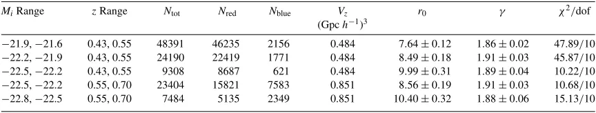
The total numbers of galaxies,Ntot, and the comoving volume,
[image:6.612.121.494.283.417.2]Figure 4.Projected correlation functions,wp(rp), for the various luminosity subsamples at low (top left) and high redshift (top right). The bottom panels present
the redshift evolution ofwp(rp) in the luminosity interval−22.8< Mi<−22.2 for all the galaxies in the sample (left) and only for the red galaxies (right). Error
bars shown are from the diagonal elements of the jackknife covariance matrices. The dotted lines in the top left panel are the power-law fits to thewpin the range of
0.1h−1Mpc< rp<2h−1Mpc to provide a guide of the small-scale slope.
[image:7.612.90.522.536.618.2](A color version of this figure is available in the online journal.)
Table 1
Samples of Different Luminosities
MiRange zRange Ntot Nred Nblue Vz r0 γ χ2/dof
(Gpch−1)3
−21.9,−21.6 0.43, 0.55 48391 46235 2156 0.484 7.64±0.12 1.86±0.02 47.89/10 −22.2,−21.9 0.43, 0.55 24190 22419 1771 0.484 8.49±0.18 1.91±0.03 45.87/10 −22.5,−22.2 0.43, 0.55 9308 8687 621 0.484 9.99±0.31 1.89±0.04 10.22/10 −22.5,−22.2 0.55, 0.70 23404 15821 7583 0.851 8.56±0.19 1.91±0.03 10.68/10 −22.8,−22.5 0.55, 0.70 7484 5135 2349 0.851 10.40±0.32 1.88±0.06 15.13/10
Notes.r0andγ are obtained from fitting a power-law towp(rp) using the full error covariance matrices for 0.1h−1Mpc< rp <
25h−1Mpc. The ratios betweenχ2and degrees-of-freedom (dof) of the fits are also shown.
3.2.2. The Dependence of Galaxy 2PCF on Luminosity
The projected 2PCFs of different luminosity samples at the two redshift bins are shown in the top panels of Figure4. At both redshifts, the luminosity dependence ofwp(rp) is evident, with more luminous galaxies exhibiting stronger clustering, consis-tent with the results of the SDSS-I/II main sample (Zehavi et al. 2005b,2011; Li et al.2006). Atz < 0.55, since red galaxies contribute 90% of the CMASS galaxy population, the
luminos-ity dependence mostly reflects the clustering environment of the red galaxies. Atz >0.55, our measurements of the 2PCF become noisier because of the lower number of galaxies. Even after accounting for the uncertainties in the measurements, the luminosity dependence of clustering is significant in the redshift range of CMASS galaxies.
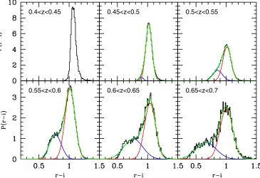
0.4<z<0.45 0.45<z<0.5 0.5<z<0.55
[image:8.612.125.490.58.308.2]0.55<z<0.6 0.6<z<0.65 0.65<z<0.7
Figure 5.Probability distribution function ofr−icolor at different redshift slices, for CMASS samples of high completeness (see text). The black lines are the histogram ofr−ifor all galaxies. The red and blue lines are the bimodality fitting using two Gaussian distributions, with the green curves as their combination. We do not fit the distribution ofr−ifor 0.4< z <0.45 because both the red and blue galaxies are far from complete in this redshift interval.
(A color version of this figure is available in the online journal.)
for more luminous samples reflects the shift in the host halo mass toward the high mass end. The modeling results in Zehavi et al. (2005b,2011) also show that the satellite fraction drops as the luminosity of galaxies increases. Our measurements naively seem to support such a result—although the 2PCFs become generally noisier for higher luminosity samples, the uncertainties in the 2PCFs on small scales increase faster. At such scales, satellite galaxies have a significant contribution to the clustering signal. Therefore, the increase in the measurement errors could be a reflection of the lack of satellites in more luminous samples.
The shapes ofwp for all luminosity samples are similar. The deviation from a power-law inwpis somewhat more apparent for brighter galaxies, consistent with the results from main galaxies (Zehavi et al.2004,2005b,2011). In the halo model, the slope of wp has a rapid change around a few Mpc, indicating the transition from intra-halo galaxy pairs (one-halo term) to inter-halo galaxy pairs (two-inter-halo term). In our measurements, we see that this transition scale increases with increasing luminosity, in agreement with the interpretation that more luminous galaxies reside in more massive (hence larger) halos. The dotted lines in the top left panel of Figure 4 show the power-law fits to
wp in the range of 0.1h−1Mpc < rp < 2h−1Mpc. There is an apparent weak trend that brighter galaxies have a steeper slope inwp on small scales, in line with the result inZ11. The dotted lines in the top left panel show the power-law fits to the
wp in the range of 0.1h−1Mpc < rp < 2h−1Mpc, the slope varies from 1.86±0.04 (the faintest sample) to 2.13±0.11 (the brightest sample). The trend can also be interpreted as a result of the change in the host halo mass scale (see Figure 7 and Appendix A in Zheng et al.2009).
The bottom panels of Figure4show the redshift evolution of the 2PCFs of galaxies in a fixed luminosity bin −22.5 < Mi <−22.2. The left panel is for all the galaxies (both blue and red). Galaxies at a lower redshift appear to have a higher
clustering strength. This result may be due to the incompleteness of blue galaxies at lower redshifts, and the inclusion of more (less clustered) blue galaxies at higher redshifts. We therefore also examine the redshift evolution of the 2PCF in the−22.5< Mi < −22.2 sample for red galaxies only, as shown in the bottom right panel of Figure 4, where the red galaxies are defined by the color cut in Equation (7). We find only slight evolution with redshift for the red galaxies (at most 18% inwp for rp > 1h−1Mpc), not significant within the measurement errors, implying that the differences in the sample of all galaxies (bottom left panel) are mostly induced by the blue galaxies.
In the redshift range of 0.16 < z < 0.44, Zehavi et al. (2005a) find no strong evolution trend inwp(rp) in the SDSS LRG sample. Their sample of −23.2 < Mg < −21.8 at 0.16< z <0.44 has a comoving number density ofn∼0.2× 10⁻⁴h3Mpc−3 (their Figure 2), similar to the number density of our sample of−22.5 < Mi < −22.2 at 0.43 < z < 0.7 shown in the bottom right panel of Figure4. Combining their results with ours, we would infer that there is no strong redshift evolution inwpof luminous red galaxies in the redshift range of 0.1< z <0.7, consistent with the results of Wake et al. (2008), implying that the effect of structure growth roughly cancels that of evolution of galaxy bias. As will be discussed in Section3.5, within the error bars, the trend is also roughly consistent with passive evolution.
3.3. Color Dependence
3.3.1. Color Cuts
Figure 6.Similar to Figure5, but for different luminosity intervals at 0.43< z <0.7. Note that blue galaxies in the leftmost panel are not complete. (A color version of this figure is available in the online journal.)
probability distribution function ofr−icolor (k+ecorrected toz=0.55) in six redshift slices as in Figure1. The distribution at each redshift is computed from galaxy samples that are as complete in luminosity as possible, i.e., we only use galaxies more luminous than the luminosity given by the intersection of line (2) and line (3) in Figure1, which corresponds to an i-band apparent magnitude of icmod = 19.46. The CMASS sample shows a clear bimodal distribution in color, similar to the findings in SDSS-I/II (Strateva et al.2001; Baldry et al. 2004; Skibba & Sheth2009). We can use the intersection of the best-fit two Gaussian distributions to divide galaxies into blue and red samples.
We do not perform the two-Gaussian fit to the galaxy distribution in redshift interval 0.4< z <0.45, as these galaxy samples are far from complete. The blue galaxies are essentially missing from this sample, and even the red galaxy colors at this redshift are not well described by a Gaussian distribution. As shown in Figure1, galaxies at this redshift suffer from thed⊥
selection cut, which eliminates the blue galaxies and a fraction of red ones. In the 0.45 < z <0.5 redshift bin, we still miss galaxies withr−i <0.9, and the distribution is dominated by the Gaussian profile from the red population. At 0.5< z <0.55, luminous blue galaxies are excluded from the sample by thed⊥
cut (see Figure1), and the contribution to the blue Gaussian profile is mainly from faint blue galaxies. Therefore, atz <0.55, blue galaxies in the CMASS sample are far from complete. For red galaxies, we find that the centers of the color distribution do not significantly change with redshift. Thus for the analysis of the whole CMASS sample, we use the redshift-independent color cut for simplicity (see Equation (7)).
The red/blue color division cut shows a mild redshift depen-dence, becoming bluer at higher redshift. Since both the color and magnitude used in this paper have beenk+ecorrected (i.e., the evolution effects are removed), such a mild evolution might indicate that the global evolution correction is not accurate. On the other hand, the photometric errors increase for larger redshift (see below), making the two Gaussian profiles broader, which can lead to a shift of the red–blue division cut toward the blue end even if there is no change in the blue and red populations. Moreover, the blue sample is generally incomplete due to the selection effects, which may also introduce additional change of the color cut. Therefore, the weak dependence of the red–blue division cut on redshift may not reveal much about the evolution. We further investigate the dependence of the color distribution on luminosity for the whole CMASS sample at 0.43< z <0.7. As shown in Figure6, the peak of the red sequence, as well as
the intersection of the two Gaussian profiles, become slightly redder as the luminosity increases, reflecting the well-known tilt of the red sequence. The tilted red sequence is likely a reflection of differences in the chemical composition, where the more luminous galaxies are richer in metals while the smaller galaxies suffer from the loss of metal-enriched gas (Kodama & Arimoto1997; Gallazzi et al.2006). The tilted red sequence may also reflect the role of dry mergers (i.e., of gas-poor galaxies) in the evolution of red galaxies (e.g., Skelton et al.2009), with galaxies increasing their mass (luminosity) from mergers and becoming older (redder) as a result of stellar evolution (see Faber et al.2007for a comprehensive review). Note that in the leftmost panel, blue galaxies are not complete in the redshift range of 0.43< z <0.7 (see Figures1and3), which leads to the non-monotonic behavior across the three panels.
In order to find a reasonable color cut for red and blue galaxies in CMASS, we fit the bimodal color distribution as a function of luminosity for galaxies in the range of 0.5< z <0.7, where the samples are less affected by incompleteness. The resulting color cut is the one already presented in Equation (7). With such a color cut, if we naively count the CMASS galaxies disregarding the incompleteness at lower redshifts, we find that only about 13% of the galaxies in CMASS are blue galaxies, and 80% of these blue galaxies are fromz >0.55. We emphasize that our color cut is based on thek+ecorrected colors.
Masters et al. (2011) proposed an observer-frame color cut of
Figure 7.Our adopted color cuts of Table2in the color–magnitude diagram. Thebc,br, andrrcuts are shown in the solid lines of colors in blue, green, and red, respectively. We ignore the redshift interval of 0.4< z <0.45 due to its high sample incompleteness.
[image:10.612.343.542.371.637.2](A color version of this figure is available in the online journal.)
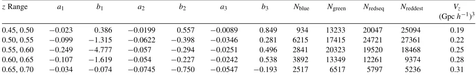
Table 2
Luminosity Dependentr−iColor Cuts for Different Redshift Intervals
zRange a1 b1 a2 b2 a3 b3 Nblue Ngreen Nredseq Nreddest Vz
(Gpch−1)3
0.45, 0.50 −0.023 0.386 −0.0199 0.557 −0.0089 0.849 934 13233 20047 25094 0.19
0.50, 0.55 −0.099 −1.315 −0.0622 −0.398 −0.0346 0.281 6215 17415 24721 27361 0.22
0.55, 0.60 −0.249 −4.777 −0.057 −0.294 −0.0251 0.496 2841 20323 19520 18468 0.25
0.60, 0.65 −0.107 −1.619 −0.054 −0.227 −0.0242 0.538 3892 13349 12261 9374 0.28
0.65, 0.70 −0.034 −0.074 −0.0745 −0.750 −0.0547 −0.193 2517 6517 5797 5236 0.31
To study the color dependence in different luminosity and redshift intervals in more detail, we further decompose the sample into finer color subsamples. The Gaussian fittings provide the centers and 1σ widths of the blue cloud and red sequence, which are used in defining the fine color cuts
(r−i)bc=blue center (15)
(r−i)br=red center−0.5×red width (16)
(r−i)rr =red center + 0.5×red width. (17)
With the three cuts, we can formblue(below thebccut),green (between thebc andbr cuts),redseq(between the brandrr
cuts), andreddest(above therrcut) samples. In each redshift interval, the luminosity-dependent color cuts are fitted with a straight line,
r−i=ajMi+bj (18)
where j = 1, 2, 3 for the bc, br, and rr cuts, respectively. The linear fits for these cuts are listed in Table2. For clarity, we show again the CMD in Figure7, with the fine color cuts superimposed. The redshift interval of 0.4 < z < 0.45 is omitted because of the high sample incompleteness.
Figure 8.1σscatter (width) of the red sequence galaxies as a function of redshift for different magnitude intervals. The solid lines are the measured scatter, and the dotted lines are the intrinsic scatter by excluding the photometric errors. The errors are only shown for one luminosity bin for clarity.
(A color version of this figure is available in the online journal.)
[image:10.612.65.546.373.452.2]Figure 9.Measurements of the 3D 2PCFξ(rp, rπ) for the blue (left panel) and red (right panel) galaxies in the whole CMASS sample, defined using the color cut in
Equation (7). Contour levels shown areξ(rp, rπ)=[0.5,1,2,5,10,20]. The dotted circles in both panels are the angle-averaged redshift-space correlation function, ξ(s), of the whole CMASS sample for the same contour values.
(A color version of this figure is available in the online journal.)
sequence as a function of luminosity and redshift. Since the photometric errors become larger for fainter galaxies and at higher redshifts, we subtract their contribution in quadrature to obtain the intrinsic color width of the red sequence galaxies. The r−i color photometric errors are estimated by simply combining in quadrature the errors inr- andi-band magnitudes (neglecting any additional errors in thek+e corrections and in the correlation betweenr- and i-band photometric errors). As shown in Figure8, the above trend persists for the intrinsic color scatter, suggesting an evolutionary effect which we discuss further in AppendixA.
3.3.2. The Dependence of Galaxy 2PCF on Color
With the color cuts defined in the previous subsection, we investigate the dependence of galaxy 2PCFs on ther−icolor. First, we examine the 2PCFs for blue and red galaxies in the whole CMASS sample. The red and blue samples here are de-fined using the color cut in Equation (7). The samples are flux-limited (in addition to other selection cuts) and are by no means complete. The purpose of this exercise is simply to have an overall view of the difference in red and blue galaxy cluster-ing. Theξ(rp, rπ) measurements for blue and red galaxies are shown in Figure9. For reference, the dotted circles in both pan-els are the angle-averaged redshift-space correlation function
ξ(s). Red galaxies are more strongly clustered. The “Fingers-of-God” feature (Jackson1972) on small scales, caused by ran-dom motions of galaxies in virialized structures, can be clearly seen for both red and blue galaxies. Red galaxies have a stronger “Fingers-of-God” effect, reflecting their stronger motions within halos. On large scales (e.g., aboverp =10h−1Mpc, the out-most contours), the contours for both blue and red galaxies show the flattening trend caused by coherent large-scale in-fall (Kaiser1987). On these scales, the Kaiser squashing effect appears to be stronger for blue galaxies, since the effect is deter-mined by≈Ω0.55
m /band blue galaxies have a smaller galaxy bias factorb.
We now investigate the color-dependent 2PCFs as a function of luminosity and redshift from the fine color samples. In order to minimize the effect of incompleteness, the luminosity and
redshift bins are selected using Figure1to make sure that red galaxies are not affected by the selection cuts. The blue galaxies are generally not complete at most redshifts and the results of the blue samples need to be interpreted with care. Nevertheless, the blue samples are still useful in comparison with the red galaxies.
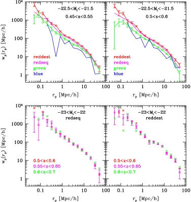
The main results of the color-dependent 2PCFs are summa-rized in Figure10. The top panels display the dependence ofwp on color in the magnitude range−22.5 < Mi <−21.5 at two different redshift intervals. The trend with color is obvious at both redshifts—there is a continuous increase in the clustering amplitude as galaxy color goes from blue to red. This result is consistent with the behavior observed in the SDSS-I/II main galaxy sample (Z11). On small scales (below the inflection scale of 1–2h−1Mpc), there appears to be a trend that redder galaxies have a steeper slope inwp, which is weaker than that measured by Z11. According to the HOD modeling result in Z11, for galaxies in a fixed luminosity range, redder galaxies generally have a higher fraction of satellites residing in massive halos. Our results therefore imply that a larger fraction of redder galaxies reside in more massive halos, giving rise to a larger clustering amplitude. The steepening of wp on smaller scales may also indicate a halo mass scale shift with color, leading to a relative increase in the contribution from the one-halo central–satellite pairs with respect to the one-halo satellite–satellite pairs (see Appendix A of Zheng et al.2009).
Figure 10.Color dependence of the projected 2PCFwp(rp). Top panels display the color dependence for the−22.5< Mi<−21.5 sample at two different redshift
intervals. The redshift evolution ofwp(rp) for theredseqandreddestsubsamples of−23< Mi<−22 galaxies is shown on the bottom.
(A color version of this figure is available in the online journal.)
3.4. Red Galaxy Samples with Fixed Number Density
In previous sections, we constructed galaxy samples in certain luminosity and color bins, in an attempt to minimize the influence of incompleteness caused by target selection cuts. Motivated by a simple passive evolution model, we can further define galaxy samples with fixed number density at different redshifts (White et al. 2007; Brown et al.2008; Wake et al. 2008). If during the evolution each galaxy in a sample retains its identity, experiencing no merger or disruption, the number density of the galaxy sample would not change with redshift. The evolution of the 2PCF of such a galaxy sample can be readily predicted (Fry1996). If, in addition, no star formation occurs in these galaxies during the process, their stellar population would evolve passively and can be readily modeled (Wake et al.2008; Tojeiro et al.2012b). Comparing to such predictions allows a rough determination of the extent of evolution in the red galaxy samples.
We construct three such samples for the red galaxies, which may be expected to resemble a passively evolving population, with fixed low, moderate and high number densities. For each sample, the fixed number density is achieved by finding a
(redshift-dependent) luminosity thresholdMi(z) and selecting all galaxies with luminosity above this threshold, as shown in Figure 11. The luminosity and redshift ranges are chosen to reduce the sample incompleteness caused by the selection cuts. The low, moderate, and high number density samples haven(z) of 0.4×10⁻⁴, 1.2×10⁻⁴, and 2×10⁻⁴h3Mpc−3, respectively. As seen in Figure 11, the fixed number density thresholds correspond globally to rough luminosity thresholds, decreasing with increasing number density as expected. The luminosity thresholds Mi(z) stay roughly constant for the red galaxies at
z > 0.48. Since the luminosities in our study have beenk+e corrected, this result implies that the stellar population in these red galaxies evolves passively. The drop belowz <0.48 is likely caused by the incompleteness of galaxies at lower redshift due to the CMASS selection cuts, as discussed in Section2.2.
Figure 11.Construction of fixed number density samples for the red galaxies, as defined by Equation (7), corresponding to low, moderate, and highn(z). The galaxies in each sample are selected by a redshift-dependent luminosity thresholdMi(z), shown in the left panel for the three samples by the blue, green and red lines,
respectively. (The two black lines delineate thei-band flux limits as in the right panel of Figure3.) The right panel shows the correspondingn(z) for the three samples, while the black solid line is the overall number density distribution of CMASS galaxies.
(A color version of this figure is available in the online journal.)
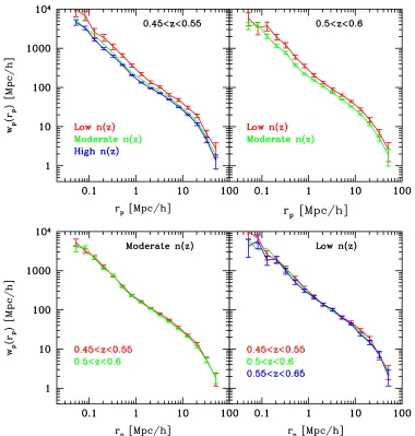
Figure 12.Projected 2PCFs,wp(rp), for fixed number density samples of CMASS red galaxies. The top panels show the dependence on number density for two
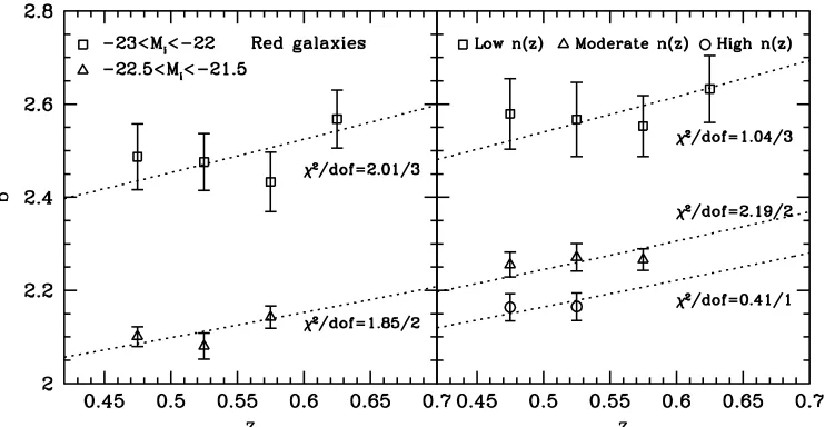
[image:13.612.116.496.315.714.2]Figure 13.Linear bias factor,b, as a function of redshift for the CMASS red galaxies in different luminosity samples (left panel) and different fixedn(z) samples (right). The symbols represent the measured galaxy biasb(z) by fittingwp(rp) over 3h−1Mpc< rp<25h−1Mpc relative to the theoretically predicted one for dark
matter. The dotted lines are the best-fit passive evolution predictions by fittingb(z) using the Fry (1996) relation. The goodness of fitχ2/dof is also given for each set
of samples.
thresholds. The shapes of the 2PCFs for differentn(z) samples are similar. The bottom panels compare the 2PCFs of the same
n(z) samples at different redshift intervals. We find that the 2PCFs at different redshifts have similar clustering strength, again consistent with the results for the luminosity dependence of red galaxies (Figure4, bottom right panel). We discuss the implications of these results next.
3.5. Galaxy Bias
With the measured galaxy 2PCFs and the theoretical matter 2PCF for the cosmology adopted in this paper, we can infer the galaxy linear bias factorbfrom the square root of the ratio between the galaxy and dark matter 2PCFs. The evolution of the linear bias factor can provide hints about the evolution of galaxy samples. In this subsection, we present the results on galaxy linear bias factorbas a function of galaxy luminosity, color, number density, and redshift, and discuss the possible implications on galaxy evolution. Since blue galaxies in the CMASS sample are generally far from complete, we will focus our discussion on the bias evolution of the red galaxies.
At each redshift, for each galaxy sample, we estimate the linear bias factorbby taking the square root of the ratio between the measured projected galaxy 2PCF and the nonlinear dark matter projected 2PCF computed at the corresponding redshift, where the latter is calculated using a modifiedhalofitmodel (Smith et al.2003) with the Eisenstein & Hu (1998) power spectrum parameterization. More specifically, we fit the ratio of galaxy and matterwp(rp) with a single parameterb on scales 3h−1Mpc< r
p<25h−1Mpc, using the full covariance matrix of the galaxywp(rp).
Fry (1996) shows that the passive evolution prediction for the linear bias factorb(z) follows
b(z)=1 +b0−1
D(z) , (19)
whereD(z) is the linear growth factor at redshiftzandb0is the bias factor atz=0 (D(0)=1). From this relation, the redshift evolution of galaxy 2PCF for the passively-evolving population
can be expressed as
ξ(z)=[b(z)D(z)]2ξm(0)=[D(z) + (b0−1)]2ξm(0), (20)
whereξm(0) is the matter 2PCF atz=0. Here we use the word “passive” to mean that during the evolution, each galaxy in the sample keeps its identity and there is no merger or disruption that changes the population. For the CMASS sample considered in this paper, the galaxy bias factor is usually greater than unity. Therefore, according to the above two equations, for passively-evolving galaxies, we expect that with decreasing redshift the amplitude of 2PCF increases while the bias factor decreases.
Figure13shows the bias redshift evolution for luminosity bin samples (left) and for the fixed number density samples (right). The bias factors are measured for non-overlapping redshift bins. The fitted bias factors support our results in the previous subsections that more luminous (or lower density) samples are more strongly clustered. The dotted lines in Figure13are the best-fit Fry (1996) relation for each sample, withb0as the single fitting parameter. For the two luminosity-bin red galaxy samples, we find that they roughly follow the passive evolution prediction. Strictly speaking, each luminosity bin sample does not conserve the number density at different redshifts. So by definition it is not a passively-evolving population. However, these number density differences may be accounted for by slightly changing the luminosity thresholds of the luminosity bin sample at each redshift (e.g., as a result of an imperfectk+ecorrection). The measured bias would not be sensitive to such an adjustment. In such a sense, comparing their bias evolution to the Fry relation can still be meaningful.
For both the luminous and faint samples, there is suggestive evidence that the clustering at intermediate redshifts (z=0.575 for the luminous sample, andz =0.525 for the faint sample) is slightly weaker than that from the best-fit passive evolution. Similar deviations from passive evolution were found in other works (e.g., White et al.2007; Wake et al.2008; Sawangwit et al. 2011). However, the large measurement errors in our results make the deviation only at about 1σ level, limiting our ability for a solid conclusion.
Figure 14.Linear bias factor,b, as a function of luminosity in two redshift ranges for all CMASS galaxies (left) and for the red galaxies only (right). The dotted curves are the bias–luminosity relation, Equation (21), withc2=0.33 for all galaxies andc2=0.35 for the red galaxies, for the lower redshift range. The dashed curve in
the right panel is the low-redshift relation shifted to the higher-redshift range according to the passive evolution prediction.
area, it would imply a significant contribution from processes that break passive evolution, such as feedback from active galactic nuclei shutting off star formation, disruption of satellites in massive halos, and mergers of galaxies (Bell et al.2004; Faber et al.2007; Skelton et al.2009). The signature may be related to the overall migration of blue galaxies to the red sequence (Martin et al.2007), in which case, it would indicate appreciable migration by z ∼ 0.55–0.6, consistent with the prediction of Faber et al. (2007). A sophisticated model is needed to disentangle the contributions from the different evolutionary processes.
The more reliable samples to study the passive evolution are the ones with fixed number densities, as described in Section3.4. The results for our three samples are shown in the right panel of Figure13. The lown(z) sample appears consistent with passive evolution in the redshift range 0.45 < z < 0.65, within the (large) error bars on the measurements. This behavior is similar to the−23< Mi <−22 sample. In fact the lown(z) sample is close to a luminosity-threshold sample of Mi < −22, as shown in Figure 11. For the two samples with higher n(z), their bias evolution is consistent with passive evolution for the smaller redshift ranges probed, which is in agreement with the conclusions of Tojeiro et al. (2012b). Within the current uncertainties, however, it is not possible to make strong statements regarding confirming or ruling out passive evolution. We will revisit this with more accurate measurements with future larger CMASS samples.
Finally, we present the dependence of the bias factor on luminosity in Figure14for all galaxies and for the red galaxies only. Generally, more luminous and redder galaxies at higher redshifts have larger bias factors. For the fainter samples, the bias factors are similar in the two cases, since at the faint end red galaxies dominate the CMASS sample (the majority of the faint blue galaxies are excluded by the selection cuts). The observed dependence of galaxy bias factor on galaxy luminosity is broadly similar to that for local galaxy samples (e.g., Norberg et al.2001; Z11), but it is non-trivial to compare in detail due to the many differences in sample selection, redshift,k+ecorrections and magnitudes.
We fit the bias-luminosity relation with a commonly-used simple functional form (Norberg et al. 2001; Zehavi et al.
2005b),
b/bp =c1+c2L/Lp. (21)
We defineLpas the mean luminosity of galaxies in the faintest luminosity bin. This sample of galaxies has b = bp, so by construction,c1 = 1−c2. We fit this functional form to the luminosity-dependent bias measurements at 0.43 < z <0.55, finding c2 = 0.33 for all galaxies andc2 = 0.35 for the red galaxies (shown as the red dotted curves in Figure14). At higher redshifts, 0.55< z <0.7, the bias factors for all galaxies show a decrease compared to the lower-redshift relation due to the inclusion of more blue galaxies at high redshifts. In contrast, the bias factors for the red galaxies globally increase with redshift, as expected from passive evolution. The dashed curve in the right panel shows the low-redshift relation shifted to high redshift according to the Fry relation prediction, which is in agreement with our measurements.
4. CONCLUSION AND DISCUSSION
In this paper, we measure the luminosity and color depen-dence of the galaxy 2PCFs based on∼260,000 BOSS CMASS DR9 galaxies over a ∼3300 deg2 survey area in the redshift range of 0.43< z <0.7 and study the implications on galaxy formation and evolution.
We first measure the 2PCF for the entire sample. If approx-imated by a power-law, the 2PCF has a correlation length of
We find that for all redshift intervals probed, more luminous galaxies are more strongly clustered, consistent with previous studies for galaxies at different redshifts, such as SDSS-I/II main sample galaxies atz ∼0.1 (Zehavi et al.2005b,2011), SDSS LRG galaxies at z ∼ 0.35 (Zehavi et al. 2005a), and DEEP2 galaxies atz∼ 1 (Coil et al.2006). At each redshift, the large-scale galaxy bias factor of CMASS galaxies shows a linear dependence on galaxy luminosity, similar to that for lower redshift galaxies (Norberg et al.2002;Z11), but with different coefficients in the bias-luminosity relation. We divide galaxies globally into a blue and a red population. For each population, we find a similar clustering trend—an increasing clustering strength with luminosity. For blue galaxies, our results are in line with that ofZ11for SDSS galaxies. For red galaxies,Z11 find that both the most luminous and faintest galaxies exhibit stronger small-scale (2h−1Mpc) clustering than the samples of intermediate luminosity, which can be explained as a large satellite fraction in the faintest sample and high mass of host halos for the most luminous sample. Because CMASS selects mostly luminous galaxies, we are not able to investigate the trend toward faint red galaxies, but for the luminous red galaxies, our results agree with that inZ11.
We further investigate the dependence of clustering on galaxy color, using finer color cuts. For fixed redshift and luminosity, we find that redder galaxies exhibit stronger clustering, similar to the trend found for the SDSS main galaxies (Zehavi et al.2005b, 2011; Li et al. 2006). Interestingly, such a trend exists even within the red sequence, consistent with the finding of Zehavi et al. (2005b,2011). The trend is different from that of DEEP2 galaxies in Coil et al. (2008), where no clear color dependence is seen across the red sequence. If this difference is caused by galaxy evolution, it implies that the color dependence in the red sequence emerges during the redshift range of 0.7 < z <1.0. The emergence of the dependence may signal the contribution of substantial amounts of mergers and inflow of blue galaxies to the buildup of the red sequence.
We also construct subsamples of red galaxies with fixed number densities by applying redshift-dependent luminosity thresholds, and compare their clustering with the theoretical prediction of passively-evolving galaxies (Fry1996). We find that the evolution of the large-scale galaxy bias factors for all the three CMASS subsamples considered in this paper are consistent with that from the Fry relation, within the relatively large uncertainties in the measured bias factors, which suggests that the red galaxies in the CMASS sample roughly follow passive evolution from z = 0.7 to 0.45. In contrast, from HOD modeling of clustering of red galaxies in NDWFS (Brown et al.2008), White et al. (2007) found that passive evolution from z ∼ 0.9 to z ∼ 0.5 would predict too many satellite galaxies in high-mass halos and concluded that about one-third of these satellites must have experienced merging or disruption. The apparent discrepancy between our result and that in White et al. (2007) can be explained by the difference in the number densities of galaxy samples. The NDWFS samples analyzed in White et al. (2007) have a constant comoving number density of
n(z) = 10−3h3Mpc−3, about one order of magnitude higher than the ones we study here. Thus, their constant number density samples include fainter red galaxies (which have a larger contribution from satellite galaxies). In contrast, galaxies in our more luminous samples are predominantly luminous central galaxies that roughly follow passive evolution (but see also Wake et al. 2008; Sawangwit et al. 2011). These results seem to support a scenario in which mergers and disruption
play an important role for the evolution of low-mass red galaxies.
Our investigation of the color–luminosity distribution at each redshift reveals two notable trends in the width of the red sequence. The red sequence becomes narrower toward the high-luminosity end, and it becomes narrower toward lower redshifts. Similar results are also seen in galaxies at both lower and higher redshifts (e.g., Bell et al.2004; Skibba & Sheth2009; Whitaker et al. 2010). The color scatter in the red sequence reflects the distribution of the ages of stellar population, dust extinction, and metallicity. At a given redshift, fainter galaxies show a more diverse distribution of these quantities, leading to a wider distribution in color. Passive evolution makes galaxies redder and largely reduces the color difference caused by the distribution of the ages of stellar population, leading to a narrower red sequence toward lower redshifts.
The inferences in this paper about the evolution of CMASS galaxies from the measured color and luminosity dependent clustering are still based on simple clustering models and interpretations. A further, natural step to interpret these results is to perform HOD modeling of our measurements, which will allow us to better study galaxy formation and evolution by incorporating knowledge about the dark matter halo formation and evolution. We expect that improved measurements from larger BOSS samples in the future and detailed HOD modeling will greatly advance our understanding of the evolution of massive galaxies.
We thank Joanne Cohn, Peder Norberg, Rom´an Scoccimarro, and Benjamin Weiner for helpful discussions. We thank the anonymous referee for useful comments. H.G., I.Z., and Z.Z. were supported by NSF grant AST-0907947. R.A.S. was sup-ported by NSF grant AST-1055081 and MECS was supsup-ported by NSF grant AST-0901965.
Funding for SDSS-III has been provided by the Alfred P. Sloan Foundation, the Participating Institutions, the National Science Foundation, and the U.S. Department of Energy Office of Science. The SDSS-III Web site ishttp://www.sdss3.org/.
SDSS-III is managed by the Astrophysical Research Con-sortium for the Participating Institutions of the SDSS-III Col-laboration including the University of Arizona, the Brazilian Participation Group, Brookhaven National Laboratory, Univer-sity of Cambridge, Carnegie Mellon UniverUniver-sity, UniverUniver-sity of Florida, the French Participation Group, the German Participa-tion Group, Harvard University, the Instituto de Astrofisica de Canarias, the Michigan State/Notre Dame/JINA Participation Group, Johns Hopkins University, Lawrence Berkeley National Laboratory, Max Planck Institute for Astrophysics, Max Planck Institute for Extraterrestrial Physics, New Mexico State Univer-sity, New York UniverUniver-sity, Ohio State UniverUniver-sity, Pennsylvania State University, University of Portsmouth, Princeton Univer-sity, the Spanish Participation Group, University of Tokyo, Uni-versity of Utah, Vanderbilt UniUni-versity, UniUni-versity of Virginia, University of Washington, and Yale University.
APPENDIX A
DIFFERENT STELLAR EVOLUTION MODELS