A tutorial introduction to Bayesian inference for stochastic
epidemic models using Approximate Bayesian Computation
Theodore Kypraios1∗, Peter Neal2, Dennis Prangle3
June 30, 2016
1 School of Mathematical Sciences, University of Nottingham, UK. 2Department of Mathematics and Statistics, Lancaster University, UK.
3 School of Mathematics and Statistics, Newcastle University, UK.
Abstract
Likelihood-based inference for disease outbreak data can be very challenging due to the inherent dependence of the data and the fact that they are usually incomplete. In this paper we review recent Approximate Bayesian Computation (ABC) methods for the analysis of such data by fitting to them stochastic epidemic models without having to calculate the likelihood of the observed data. We consider both non-temporal and temporal-data and illustrate the methods with a number of examples featuring different models and datasets. In addition, we present extensions to existing algorithms which are easy to implement and provide an improvement to the existing methodology. Finally, R code to implement the algorithms presented in the paper is available on https://github.com/kypraios/epiABC.
1
Introduction
The past two decades have seen a significant growth in the field of mathematical modelling of communicable diseases and this has led to a substantial increase in our understanding of infectious-disease epidemiology and control. Understanding the spread of communicable infec-tious diseases is of great importance in order to prevent major future outbreaks and therefore it remains high on the global scientific agenda, including contingency planning for the threat of a possible influenza pandemic. The main purpose of this paper is to give an introduction and overview of some of the recent work concerned with Approximate Bayesian Computation methods for performing (approximate) Bayesian inference for stochastic epidemic models given data on outbreaks of infectious diseases. In addition, we present novel modifications to the existing algorithms and show that such modifications can be more efficient than the existing state-of-the-art algorithms. In the present section we discuss generic ideas with the bulk of the remainder of the paper containing various algorithms and illustrative examples.
1.1 Models and Inference for Epidemic Models
It has been widely recognised that mathematical and statistical modelling has become a valuable tool in the analysis of infectious disease dynamics by supporting the development of control
∗
strategies, informing policy-making at the highest levels, and in general playing a fundamental role in the fight against disease spread (Hollingsworth, 2009).
The transmissible nature of infectious diseases makes them fundamentally different from non-infectious diseases, and therefore the analysis of disease outbreak data cannot be tackled using standard statistical methods. This is mainly due to the fact that the data are i) highly dependent and ii) incomplete, in many different ways since the actual transmission process is not directly observed. However, it is often possible to construct simple stochastic models which describe the key features of how an infectious disease spreads in a population. The complexity of the models typically varies depending on the application in question as well as the data available. For example, models may incorporate a latent period during which individuals are infected but not yet infectious, reduced infectivity after control measures are imposed, etc. Similarly, aspects of the population heterogeneity can also be included such as age structure and that individuals live in households and go to workplaces, etc.
Models can then be fitted to data either within a classical or Bayesian framework to draw inference on the parameters of interest that govern transmission. In turn these parameters can be used to provide useful information about quantities of clinical or epidemiological interest. One needs always to strike a balance between model complexity and data availability. In other words, it is not wise to construct a fairly complicated model when not much data are available and vice versa.
1.2 Bayesian Inference
In frequentist inference, model parameters are regarded as fixed quantities. On the other hand, a Bayesian approach treats all the unknown model parameters as random variables, enabling us to quantify the uncertainty of our estimates in a coherent, probabilistic manner. The Bayesian paradigm to inference operates by first assigning to the parameters a prior distribution which represents our belief about the unknown parameters (θ) before seeing any data. Subsequently this prior information is updated in the light of experimental data (D) using Bayes theorem by multiplying it with the likelihood π(D|θ) and renormalising, thus leading to the posterior distribution π(θ|D) via:
π(θ|D) = R π(D|θ)π(θ) θπ(D|θ)π(θ)dθ
∝π(D|θ)π(θ). (1)
All Bayesian inference arises from the posterior distribution in the sense thatπ(θ|D) contains all the information regarding our knowledge about the parameters θ given the experimental data D and any prior knowledge which might be available. Point and interval summaries of the posterior distribution (such as mean, median and credible intervals) can easily be obtained. The advantage of a Bayesian approach as opposed to a frequentist inference is that the former enables the complete quantification of our knowledge about the unknown parameters in terms of a probability distribution. We highlight such advantages in subsequent Sections.
1.3 Approximate Bayesian Computation
as Approximate Bayesian Computation (ABC) allows us to perform inference without having to compute the likelihood.
We have already mentioned above that one of the difficulties when fitting models to disease outbreak data is that the infection process is unobserved. The likelihood of the observed data can become very difficult to evaluate and so is the posterior distribution. This is particularly the case when analysing temporal data, since calculating the likelihood involves integration over all possible infection times, which is rarely analytically possible. On the other hand, simulating realisations from a stochastic epidemic model is relatively straightforward. Therefore, ABC algorithms are very well suited to make inference for the parameters of epidemic models based on partially observed data and this has been illustrated when both temporal (McKinley et al., 2009) and non-temporal data Neal (2012) are available.
1.4 Other Approaches to Inference
One way to overcome this issue is to employ data imputation methods where unknown quantities (such as the infection times) are treated as additional model parameters and inferred along with the other parameters. One of the most widely used methods for doing so is Markov Chain Monte Carlo (MCMC) which have revolutionised not only Bayesian statistics, but have also been developded for fitting stochastic epidemic models to partially observed outbreak data (O’Neill and Roberts, 1999; Gibson and Renshaw, 1998). Despite being successfully applied to a wide variety of applications such as Foot-and-Mouth (Streftaris and Gibson, 2004; Chis-Ster and Ferguson, 2007; Kypraios, 2007), SARS outbreaks (McBryde et al., 2006), healthcare-associated infections (such as MRSA and C. difficile) (Forrester et al., 2007; Kypraios et al., 2010) and Avian, H1N1 and H3N2 influenza (Jewell et al., 2009a; Cauchemez et al., 2004, 2009) as the population size increases and/or the model becomes more sophisticated, the likelihood can become prohibitively costly to compute. In addition, non-standard and problem-specific MCMC algorithms need to be designed to improve on the efficiency of the standard algorithms. The remainder of the paper is structured as follows. In Section 2, we introduce the ABC algorithm including extensions to ABC-MCMC and sequential based ABC-PMC. In Section 3, we apply the ABC algorithm to non-temporal (final outcome) data, firstly to a homogeneously mixing SIR epidemic model and secondly to a household SIR epidemic model. For the latter we introduce a new partially coupled ABC algorithm which offers significant gains in efficiency. In Section 4, we turn to the analysis of temporally observed epidemic data, in particular, the effective implementation of adaptive ABC-PMC algorithms.
2
ABC Algorithms
Intuitively, ABC methods involve simulating data from the model using various parameter values and making inference based on which parameter values produced realisations that are “close” to the observed data. Algorithm 1 generates exact samples from the Bayesian posterior density
Algorithm 1 Exact Bayesian Computation (EBC)
Input: observed dataD, parameters governing π(θ)
Output: samples from π(θ|D) 1. Sampleθ∗ from π(θ).
2. Simulate datasetD∗ from the model using parametersθ∗. 3. Acceptθ∗ ifD∗=D, otherwise reject.
4. Repeat until the required number of posterior samples is obtained.
This algorithm is only of practical use ifDis discrete, else the acceptance probability in Step 3 is zero. For continuous distributions, or discrete ones in which the acceptance probability in step 3 is unacceptably low, Pritchard et al. (1999) suggested the following algorithm:
Algorithm 2 Approximate Bayesian Computation (vanilla ABC)
Input: observed dataD, tolerance , distance function d(·,·), summary statisticss(·), parame-ters governingπ(θ)
Output: samples from ˜π(θ|D) =π(θ|D, d s(D), s(D∗)≤ε) 1. Sampleθ∗ from π(θ).
2. Simulate datasetD∗ from the model using parametersθ∗. 3. Acceptθ∗ ifd s(D), s(D∗)≤ε, otherwise reject.
4. Repeat until the required number of posterior samples is obtained.
Here,d(·,·) is a distance function, usually taken to be theL2-norm of the difference between its arguments; s(·) is a function of the data; and ε is a tolerance. Note that s(·) can be the identity function but in practice, to give tolerable acceptance rates, it is often the case that it is a lower-dimensional vector comprising summary statistics that characterise key aspects of the data. In addition, if the prior and the posterior distribution are rather different, for example, in the case where the data are very informative about the model parameters then the rejection sampling approach of this ABC algorithm will be very inefficient. A wide range of extensions to the original ABC (which is often termed vanilla ABC) algorithm have been developed over the past decade and it still remains a topic of significant research interest.
2.1 Summary Statistics
As discussed above, using s(·) as the identity function gives an inefficient ABC algorithm if the data is high dimensional. The underlying reason is a curse of dimensionality issue. Roughly speaking, for a fixed computational cost the quality of the ABC output sample as an approxi-mation of the posterior deteriorates as the number of summaries, p, increases. This is the case even taking into account the possibility of adjusting .
The problem is that simulations which produce good matches of all summaries simultaneously become increasingly unlikely aspgrows. A formal treatment of the issue is given by Blum (2010), Barber et al. (2015) and Biau et al. (2015) amongst others.
Hence for ABC to produce a useful approximation of the posterior, a careful choice of s(·) is required which balances informativeness and low-dimensionality. Many methods for selecting summary statistics have been proposed. See Blum et al. (2013) and Prangle (2015b) for reviews of these methods and more discussion of the points above.
In this paper we make use of a sufficient statistic when analysing final outcome data, and in the cases where no low order sufficient statistics are available, we use intuitively chosen summary statistics such as sum-of-squared differences between observed and removal counts in several time intervals and the duration of the epidemic.
2.2 ABC-MCMC
To overcome issues caused by a low acceptance probability when the prior and posterior distri-butions are rather different Marjoram et al. (2003) developed an algorithm that embeds the sim-ulation steps into a standard Metropolis–Hastings (M-H) Markov Chain Monte Carlo (MCMC) algorithm (henceforth, ABC-MCMC).
Algorithm 3 Approximate Bayesian Computation Markov Chain Monte Carlo
(ABC-MCMC)
Input: observed dataD, tolerance , distance functiond(·,·), summary statisticss(·), proposal distribution q(·|·), parameters governing π(θ), initial state θ0
Output: samples from ˜π(θ|D) 1. Letθc=θ0.
2. Sampleθ∗ from a proposal distribution q(·|θc).
3. Simulate K datasets D∗1, . . . , DK∗ from the model using parametersθ∗ and calculate
r(D, θ∗) = 1
K K X
k=1
I d s(D), s(Dk∗)
≤ε
whereI(E) = 1 if E is true, and 0 otherwise.
4. Acceptθ∗ with probability
min
1,r(D, θ ∗)
r(D, θc) π(θ∗)
π(θc)
q(θc|θ∗)
q(θ∗|θc)
5. Ifθ∗ is accepted, then setθc=θ∗. 6. Record the current state.
7. Go to Step 2 and repeat until the required posterior samples are obtained.
The ABC-MCMC algorithm is very similar to the standard M-H algorithm. The only, but crucial, difference is in the acceptance probability ratio. In the standard M-H algorithm one has the ratio of the likelihoods evaluated at the candidate and the current value of the Markov chain, whist in ABC-MCMC the likelihood terms are each approximated by the proportion of
faced with when using ABC-MCMC is selecting the and ktuning parameters, which typically requires expensive pilot runs.
2.3 ABC-PMC
Several authors have developed algorithms which embed ABC simulation steps in Sequential Monte Carlo (SMC) algorithms. The idea is to sample from a sequence of approximate ABC posteriors under successively lower acceptance tolerances. The sample from one iteration, known as particles, is used to help choose which θvalues to simulate from in the next. SMC methods for ABC have a number of potential advantages over MCMC and vanilla ABC. Unlike vanilla ABC they concentrate on simulating datasets from θ regions with relatively high acceptance probabilities, avoiding wasting computational resources. Unlike MCMC, they can adapt tuning choices, such as acceptance tolerances, during their operation.
In this paper we concentrate on the widely used algorithm of Toni et al. (2009), Algorithm 4. This effectively performs repeated importance sampling, also known aspopulation Monte Carlo (Capp´e et al., 2004). We therefore refer to this as the ABC-PMC algorithm. There is also a wider family of related ABC-SMC algorithms, including Sisson et al. (2007) and Del Moral et al. (2012), which update their particles in more complex ways based on MCMC moves, as described in Del Moral et al. (2006).
Algorithm 4 Approximate Bayesian Computation Population Monte Carlo
(ABC-PMC)
Input: observed data D, number of intermediate distributions M, number of tolerances
1, . . . , M, distance functiond(·,·), summary statisticss(·), number of particlesN, kernelK(·|·),
parameters governing π(θ)
Output: weighted samples from ˜π(θ|D) 1. Lett= 1.
2. Repeat the following steps until there areN acceptances.
(a) Sampleθ∗ from the importance densityqt(θ) given in (2) below.
(b) Ifπ(θ∗) = 0 reject and return to (a).
(c) Simulate datasetD∗ from the model using parametersθ∗.
(c) Acceptθ∗ ifd s(D), s(D∗)
≤εt
Denote by θt1, θt2, . . . , θtN the accepted parameter values. 3. Letwt
i =π(θti)/qt(θti) fori= 1,2, . . . , N.
4. Incrementt=t+ 1.
5. Repeat Steps 2 and 3 until t=M.
6. Return final accepted samples and corresponding weights.
The importance density in Step 2a) is given by
qt(θ) =
π(θ) ift= 1,
PN i=1w
t−1
i Kt(θ|θti−1)/ PN
i=1w
t−1
i otherwise.
In other words, in the first iterationqt(θ) is the prior and for the subsequent iterations, weighted
samples from the previous particle population are drawn and the perturbed using the kernelKt.
The choice of the kernel is arbitrary but Beaumont et al. (2009) illustrate that a good choice is
K(θt|θt−1) =φ θt−1,2Σt−1
(3)
where φ(·,·) is the density of a (multivariate) Normal distribution and Σt−1 is the empirical covariance matrix of the particle population at timet−1,{θit−1}1≤i≤N, calculated using weights
{wit−1}1≤i≤N.
One common variation on Algorithm 4 (Drovandi and Pettitt, 2011), which we will use in this paper, is to determine the sequence of tolerances adaptively during the algorithm. To do so one selects an initial tolerance, such as 1 =∞, and then selectst+1 between steps 3 and 4. The value used is theα quantile ofdt1, dt2, . . . , dtN, where these are thed s(D), s(D∗) distances from the accepted simulations at time t, and 0< α <1 is a tuning parameter.
We found that adaptive tolerances sometimes perform poorly for discrete summary statis-tics, which several of our applications use. The problem occurs when most of the distances from accepted simulations exactly equal the tolerancet. In practice, these typically correspond
to simulated epidemics in which no infections occur. Then t+1 = t and the algorithm
be-comes stuck at this tolerance level. To fix this issue we change the acceptance condition to
d(s(D), s(D∗)) < i.e. using a strict inequality. This guarantees that the tolerances form a strictly decreasing sequence.
3
ABC for Non-Temporal Data
3.1 Introduction
3.2 Homogeneously mixing SIR epidemic model
We use the so-called homogeneously mixing Susceptible-Infective-Removed (SIR) epidemic model to illustrate the strengths and weaknesses of the ABC algorithm and to introduce extensions to the ABC methodology. As we shall see in Section 3.4 these extensions are applicable to more general epidemic models.
3.2.1 Definition
We begin by describing the SIR model in a homogeneously mixing population. Suppose that we have a closed population of N individuals. Suppose that one individual is infected from outside the population and initiates an epidemic within the population with no further external infections. The remaining N −1 individuals in the population are initially susceptible and the epidemic progresses as follows. Infectious individuals have independent and identically distributed infectious periods according to a random variableI, whereI is assumed to belong to some known family of probability distributions, possibly with unknown parameters to estimate. Whilst infectious individuals make infectious contacts at the points of a homogeneous Poisson point process with rate λ. Each infectious contact is with an individual chosen uniformly at random from the entire population. If the contacted individual is susceptible, they become infected and immediately infectious. Infectious contacts with non-susceptible individuals have no effect on the recipient. At the end of their infectious period, an individual becomes removed, either recovery followed by immunity or in severe cases death, and plays no further role in the epidemic. The epidemic ends when there are no more infectives in the population and the total number of removed individuals denotes the final size of the epidemic.
3.2.2 Simulation
Simulation of the epidemic process is trivial, if we are only interested in the final size of the epidemic, as we do not need to consider the time course of the epidemic. In particular, we can consider in turn the set of individuals infected by a given infective. The number of infectious contacts made by an infective follows a mixed Poisson distribution with meanλI. The probabil-ity that an infectious contact is successful (infects a susceptible individual) is S/N, where S is the current number of susceptibles. Each infection leads to the number of susceptibles decreas-ing by one and the number of infectives increasdecreas-ing by one. Once we have considered the set of infections made by an infective, the infective becomes removed and we decrease the number of infectives by one. The simulation ends when there are no more infectives in the population.
For the coupled ABC algorithm and other extensions of the ABC algorithm which exploit non-centered parameterisations (Roberts et al., 2003), it is helpful to use the alternative but equivalent Sellke (Sellke, 1983) construction of the epidemic process. That is, every initially susceptible individual in the population is assigned an independent and identically distributed infectious threshold, T ∼ Exp(1/N). Then individual i becomes infectious when the total amount of infectious pressure exceeds Ti, where the infectious pressure exerted by an infective j, with infectious period Ij is λIj. As noted in Sellke (1983) and Neal (2012), it is helpful to
consider the ordered thresholds,T(1)(= 0)< T(2)< . . . < T(N), whereT(1) denotes the threshold of the initial infective. It is straightforward to show that, for i = 1,2, . . . , N −1, T(i+1) − T(i) ∼ Exp((N −i)/N). Thus if we let L1, L2, . . . , LN−1 be independent exponential random variables with Li ∼Exp((N−i)/N), we can simulate a realisation of the ordered thresholds by
I = (I1, I2, . . . , IN), then the final sizeMλ of an epidemic with parameterλsatisfies
Mλ= min
m: (T(m+1) =)
m X
i=1
Li > λ m X j=1 Ij . (4)
Algorithm 5 illustrates this procedure to simulate the final size by exploiting the Sellke con-struction.
Algorithm 5 Simulation of the final size of a homogeneously mixing SIR model
Input: population sizeN, infection rateλ, parameters governing f(I)
Output: final size
1. Simulate I1, I2, . . . , IN independently from the infectious period distributionf(I).
2. Simulate L1, L2, . . . , LN−1 independently with eachLi ∼Exp NN−i
,i= 1, . . . , N−1. 3. Calculate the ordered thresholds T(i) =
Pi−1
j=1Lj,i= 1, . . . , N.
4. Find the final size Mλ using Equation (4).
It is worth noting for the homogeneously mixing SIR epidemic the final size of the epidemic is a one dimensional sufficient statistic as for inference it does not matter which individuals are infected, only how many individuals are infected. Therefore it is trivial to implement an EBC algorithm 1 which produces exact samples from the true posterior distribution of the infection rate.
3.3 Coupled ABC algorithm
The coupled ABC algorithm exploits the non-centered parameterisation underpinning (4). That is, we can simulate L and I independent of λand we can use the same L and I with different choices of λ to simulate epidemics. The coupling terminology comes from probability theory, see for example Lindvall (1992), and here indicates that if λ1 < λ2 then using the sameL and I, we get Mλ1 ≤Mλ2. Moreover, we can consider epidemics for all values of λ∈ R
+ using L and I with
λ∈
max
1≤k≤m−1
k X i=1 Li , k X j=1 Ij , m X i=1 Li , m X j=1 Ij
, (5)
generating an epidemic with final size m. Note that often the set on the right hand side of (5) will be empty with an epidemic which infects at least m individuals infecting at least m+ 1 individuals.
Suppose that we observe a final sizeDand the infection rateλfollowsa prioria distribution with probability density function π(λ). An EBC algorithm (Algorithm 1) to sample from the posterior distribution of λis very straightforward to apply. One can also easily apply the ABC algorithm (Algorithm 2) where the requirement of an exact match of the final size between the observed and simulated is relaxed. To implement the coupled ABC algorithm (see Algorithm 6 below), we first generate T independent copies of L andI and fort= 1,2, . . . , T, let
At=
max
1≤k≤D−1
k X i=1 Li , k X j=1 Ij , D X i=1 Li , D X j=1 Ij
denote the set of λvalues consistent with an epidemic of sizem from the tth realisation. Thus far we have not mentioned the prior distribution with regards the coupled ABC algorithm. For
t= 1,2, . . . , T, let
wt= Z
At
π(λ)dλ, (7)
denote the weight attached to simulation t. Note that wt is the probability that a value of λ
drawn from the prior combined with the tth realisation ofL and I results in an epidemic with final sizeD. Thus we have sets (At) ofλvalues from the posterior distribution with associated
weights (wt). These can be used directly to compute posterior moments. For example,
ˆ φ= T X t=1 Z At
λπ(λ)dλ , T
X
t=1
wt (8)
is a consistent estimator of E[λ|m]. Alternatively, we can use {(At, wt)} to generate a sample
of size K from the posterior distribution, by for k= 1,2, . . . , K, sampling I from {1,2, . . . , T} withP(I =t)∝wtand then samplingλk fromAI using rejection sampling (see Neal (2012) for
details).
Algorithm 6 Coupled-ABC algorithm for a homogeneously mixing SIR model
Input: final sizeD, population sizeN, infection rate λ, parameters governing π(λ)
Output: Moments of π(λ|D)
1. GenerateT independent copies ofL and I. 2. Fort= 1, . . . , T find the sets At:
At=
max
1≤k≤D−1
k X i=1 Li , k X j=1 Ij , D X i=1 Li , D X j=1 Ij .
3. For eacht= 1, . . . , T calculate the weightswt= R
Atπ(λ)dλ.
4. Compute a Monte Carlo estimate of the posterior mean of λ:
\
E[λ|D] = PT1
t=1wt T X
t=1
Z
At
λπ(λ)dλ
5. Compute the posterior variance of λ:
\
V[λ|D] = PT1
t=1wt T X
t=1
Z
At
λ2π(λ)dλ−E\[λ|D]2
3.3.1 Application to the Abakaliki smallpox outbreak
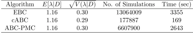
population ofN = 120. We assume an Exp(1) prior forλand thatI ∼Exp(1). Similar results are obtained withI ≡1 andI ∼Gamma(2,2) and aU(0,5) prior forλ, see Neal (2012), except for the acceptance rates of the ABC algorithms which are sensitive to prior choice. The more uninformative the priors are, of course, the lower the acceptance rates will be. Note that for the coupled ABC acceptance of a simulation is independent of the prior distribution. For the ABC and coupled ABC algorithms we ran the algorithms until we got 10000 accepted values, accepting only those simulations which resulted in an exact match. In other words, we are drawing samples from the exact posterior distribution of λ given the data D. For the ABC-PMC we ran the algorithm with M = 2 tolerance levels and = (10,0) with each tolerance level run until 10000 accepted values are generated. For each algorithm we report the estimated posterior mean and standard deviation of λalong with the number of simulations and time (in seconds) required to obtain the results in Table 1.
Algorithm E[λ|D] pV(λ|D) No. of Simulations Time (sec)
EBC 1.16 0.30 13064009 3355
cABC 1.16 0.29 177887 169
[image:11.595.129.461.283.340.2]ABC-PMC 1.16 0.30 6607900 2643
Table 1: Comparison of ABC algorithms for the Abakiliki data set
The results demonstrate that the coupled ABC algorithm performs substantially better than the other ABC algorithms. The improvements offered by the ABC-PMC over the ABC are modest, due primarily to the prior giving significant support to λ values between 0.8 and 1.6 where the majority of the posterior distribution lies. The ABC-PMC algorithm gives a far more substantial improvement if a more diffuse prior for λis chosen. The reason for only using two tolerance levels for the ABC-PMC is that similar values of λare responsible for epidemics infecting between 20 and 40 individuals thus there is no gain by inserting intermediary tolerances. In fact the estimated posterior mean and standard deviation using ABC and a tolerance of 10 (accepting simulations producing epidemics between 20 and 40 individuals) were 1.15 and 0.31, respectively, and required 564563 simulations in 145 seconds.
3.4 Household SIR epidemic model
3.4.1 Definition
An important class of epidemic models are the household epidemic models; see Ball et al. (1997). We consider a population of N individuals whom are partitioned into H households. Let K denote the maximum household size with for k = 1,2, . . . , K, Hk households of size k. Thus H = PKk=1Hk and N = PKk=1kHk. As for the homogeneously mixing epidemic we
assume that individuals are independent and identically distributed in terms of their infectious behaviour should they become infected with an infectious period I. During their infectious period individuals can make infectious contacts with any member of the population but are assumed to have increased contact with members of their own household. Specifically, infectious individuals makeglobalinfectious contacts at the points of a homogeneous Poisson point process with rateλG, during their infectious period, with the individual contacted chosen uniformly at
point process with rate λL/(di −1)α, where di is the size of individual i’s household and α
is a power parameter determining the effect of household size on epidemic transmission. Note that α = 0 and α = 1 correspond to density-dependent and frequency-dependent transmission within households, respectively, and ifλL= 0 we essentially return to the homogeneously mixing
epidemic model introduced above.
3.4.2 Simulation
For simulation of the household epidemic model, especially for using the coupled ABC algorithm, it is useful to again use a Sellke construction of the epidemic process, see for example Ball et al. (1997) and Neal (2012). Since the time course of the epidemic is not important for non-temporal data, we follow Ball et al. (1997) in considering the local epidemic (within household) generated by a global infection before considering the next global infection. An individual is chosen at random to be the initial infective. This individual instigates an epidemic in their household which results in Y1 individuals (including the initial infective) being infected with severity (sum of the infectious periods of the individuals) being S1. For j = 1,2, . . ., (Yj, Sj)
denotes the number of individuals infected and the corresponding severity from the within household epidemic emanating from the jth global infection. Note that the {(Yj, Sj)}’s will be
independent but will depend upon the size of the household and the number of susceptibles in the household prior to the jth global infectious contact. The Sellke construction for the
homogeneously mixing epidemic with minor modifications to take into account the number of susceptibles in a household at the start of a local epidemic can be used to simulate (Yj, Sj). We
now turn to the global infections. For i= 1,2, . . . ,let
Li ∼Exp
N−
i X
j=1 Yj
/N
. (9)
Then Li gives the additional amount of global infectious pressure required after the ith global
infection for the (i+ 1)st global infection to occur, given that the local epidemics instigated by the first iglobal infections are taken account of. Then letting T(i) =
Pi−1
j=1Lj (i= 1,2, . . .), the global infectious thresholds, we have that the total number of global infections (including the initial infective) with global infection rate λG is
MλG= min
m: (T(m+1) =)
m X
i=1
Li > λG m X
j=1 Sj
. (10)
The key observation is that (10) is virtually identical to (4). The only differences are that the sum of the infectious periods of the first m infectives is replaced by the sum of the severities of the firstm local epidemics and thatLi depends upon how many individuals infected in the first i local epidemics which in the homogeneously mixing case is simply i. Thus those individuals infected during the course of the epidemic are those infected by the firstMλG global infections
or resulting local epidemics.
3.4.3 A Partially coupled ABC algorithm
and subsequently the thresholds L. Then Land S, combined with λG in the range
max
1≤k≤m−1
k X
i=1 Li
, k
X
j=1 Sj
,
m X
i=1 Li
, m
X
j=1 Sj
(11)
will result in an epidemic which hasmglobal infections. As before, often (11) will be empty with an epidemic which leads to at leastm global infections having at least m+ 1 global infections.
Algorithm 7 Partially coupled ABC algorithm for household epidemics
Input: observed dataD, tolerances 1 and 2, parameters governingπ(λL),π(λG) and π(α)
Output: Weighted samples from an approximateπ(λL, λG, α|D).
1. Initialise xwhich will keep track of the state of the epidemic following each global infection with xij being the number of households of size j with i individuals infected. Initially all
individuals are susceptible with Hi (the number of households of size i) being set equal to
the number of households of sizeiin the observed data x∗.
2. SampleλLfrom its prior distributions and set the value ofαto be fixed at 0 or 1 if a density
or frequency dependent infection model for households is assumed. Alternatively, sampleα
from a prior distribution if it is not chosen to be fixed. 3. Forj = 1, . . . , N:
(a) Simulate local epidemic (Yj, Sj) with the individual chosen for thejthglobal infection
chosen uniformly at random from the set of remaining susceptibles following the (j− 1)st infection.
(b) Update x to take into account the jth local epidemic and record δj = |x−x∗|, the
distance between the simulation after the jth global infection and the observed data.
(c) Simulate Lj ∼Exp({N−Pij=1Yj}/N).
(d) Use Equation 11 to compute the range ofλGvalues which will result in exactlyjglobal
infections.
(e) If δj ≤ 1, |Pji=1Yi−PHk=1PHl=0l xlk| ≤ 2 and the set of λG values is non-empty,
store the information for the simulation; parameters (λG, λL, α) and the precisions
(δj,Pji=1Yi −PHk=1
PH
l=0l xlk). Note that at most N global infections are required
for everybody in the population to be infected.
In Neal (2012), a coupled ABC algorithm is given which simultaneously considers all choices of (λG, λL) for fixed α (implicit in Neal (2012), α = 0). Whilst the coupled ABC algorithm
has a higher acceptance probability than the partially coupled ABC algorithm, it is far more computationally intensive, both in coding and implementation taking approximately 20 times longer per iteration (see Neal (2012)) and is thus not worth the extra effort. The cost of the partially coupled ABC algorithm over a vanillaABC algorithm is relatively small since in both cases the same procedures are followed except that the simulation of the standard ABC algorithm stops after the Mth
3.4.4 Application to outbreak data in households
We demonstrate the capabilities of the various ABC algorithms using household final size data from four influenza outbreaks (two from Seattle, Washington and two from Tecumseh, Michigan, reported in Fox and Hall (1980) and Longini et al. (1982), respectively) previously studied by and given in Clancy and O’Neill (2007) and Neal (2012). For comparison with earlier work we assume a constant infectious periodI ≡1 and we assume Exp(1) priors for the infection ratesλGandλL.
Both Clancy and O’Neill (2007) and Neal (2012) reportqG= exp(−λGQ/N) andqL= exp(−λL),
where Q is the final size of the epidemic. Note that qG and qL are the probabilities that an
individual avoids a global infection throughout the course of the epidemic and that an individual avoids a local infection from a given infective in their household, respectively. Thus we report estimates of the means and standard deviations ofqGand qLin the main text with estimates of
the means and standard deviations of λG and λL provided in the Supplementary Material B.
It is straightforward to implement a PMC version of the partially coupled ABC algorithm which uses an updated proposal distribution forλLat each stage of the PMC algorithm. Details
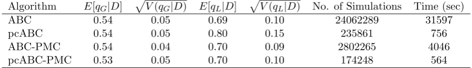
of a generic PMC algorithm for partially coupled ABC is provided in the Supplementary Material A. Therefore we have four algorithms to compare vanilla ABC, ABC-PMC, partially coupled ABC and the partially coupled ABC-PMC. In all cases the algorithms were run to obtain 1000 accepted values with two intermediary stages used for the PMC algorithms. As noted in Neal (2012), requiring an exact match leads to an unacceptably low acceptance probability therefore we use the same data set dependent thresholds used in Neal (2012). For each algorithm we report the estimated posterior mean and standard deviation of (qG, qL) along with the number
of simulations and time (in seconds) required to obtain the results in Tables 2, 3, 4 and 5 for the Seattle influenza A, Seattle influenza B, Tecumseh 1977-8 outbreak and Tecumseh 1980-1 outbreak, respectively. The results show that the vanilla ABC performs very poorly compared with the other algorithms taking more than 250 times as long as the partially coupled ABC-PMC algorithm to obtain comparable results for both of the Tecumseh outbreaks. The partially coupled ABC-PMC algorithm is the most efficient taking approximately two-thirds of the time of the partially coupled ABC algorithm without any effort to optimise the PMC algorithm and for the same set of stages is approximately ten times faster than the standard ABC-PMC algorithm.
Algorithm E[qG|D] p
V(qG|D) E[qL|D] p
V(qL|D) No. of Simulations Time (sec)
ABC 0.54 0.05 0.69 0.10 24062289 31597
pcABC 0.54 0.05 0.80 0.15 235861 756
ABC-PMC 0.54 0.04 0.70 0.09 2802265 4046
[image:14.595.69.542.522.591.2]pcABC-PMC 0.53 0.05 0.70 0.10 174248 564
Algorithm E[qG|m] p
V(qG|m) E[qL|m] p
V(qL|m) No. of Simulations Time (sec)
ABC 0.84 0.03 0.84 0.06 14905586 32952
pcABC 0.84 0.03 0.84 0.07 232796 393
ABC-PMC 0.84 0.03 0.84 0.07 2967606 3362
[image:15.595.71.542.108.177.2]pcABC-PMC 0.84 0.03 0.84 0.06 151319 282
Table 3: Comparison of ABC algorithms for the Seattle influenza B data set with = (20,2) and intermediary thresholds = (50,5) and = (30,3) for the ABC-PMC algorithm.
Algorithm E[qG|m] p
V(qG|m) E[qL|m] p
V(qL|m) No. of Simulations Time (sec)
ABC 0.86 0.02 0.84 0.06 38126827 229535
pcABC 0.86 0.02 0.84 0.06 339775 1334
ABC-PMC 0.86 0.02 0.84 0.06 5077091 14196
[image:15.595.69.544.253.322.2]pcABC-PMC 0.86 0.020 0.84 0.06 190664 906
Table 4: Comparison of ABC algorithms for the Tecumseh 1977-8 outbreak data set with = (50,4) and intermediary thresholds= (100,10) and = (70,6) for the ABC-PMC algorithms.
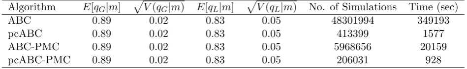
Algorithm E[qG|m] p
V(qG|m) E[qL|m] p
V(qL|m) No. of Simulations Time (sec)
ABC 0.89 0.02 0.83 0.05 48301994 349193
pcABC 0.89 0.02 0.83 0.05 413399 1577
ABC-PMC 0.89 0.02 0.83 0.05 5968656 20159
pcABC-PMC 0.89 0.02 0.83 0.05 206031 928
Table 5: Comparison of ABC algorithms for the Tecumseh 1980-1 outbreak data set with = (50,4) and intermediary thresholds = (100,10) and= (70,6) for the ABC-PMC algorithm.
4
ABC for Temporal Data
[image:15.595.69.544.398.469.2]4.1 Definition
It is fairly straightforward to simulate temporal realisations from a homogeneously mixing SIR model since it can be viewed as a bivariate Markov process {S(t), I(t) : t ≥ 0} in continuous time where (S(0), I(0)) = (N −1,1) and with the following transition rates:
(i, j)→(i−1, j+ 1) : λ
NS(t)I(t)
(i, j)→(i, j−1) : γI(t)
and the corresponding transition probabilities to an infection and removal:
P[S(t+δt)−S(t) =−1, I(t+δt)−I(t) = 1| Ht] = λ
NS(t)I(t) +o(δt)
P[S(t+δt)−S(t) = 0, I(t+δt)−I(t) =−1| Ht] = γI(t) +o(δt).
All other transitions having probability o(δt) and Ht is the sigma-algebra generated by the
history of the process up to time t.
4.2 Simulation
A continuous time Markov chain can be simulated using next event simulation, often called the Gillespie algorithm (Gillespie, 1977). All that is needed is to generate the time the Markov chain spends in a state and the next state that it visits. Recall that each infectious individual remains so for a length time TI ∼Exp(γ) and during this time, infectious contacts occur with
each susceptible according to a Poisson process with rate Nλ. Thus the overall infection rate is
λ
NS(t)I(t).
Algorithm 8 Simulation of temporal data from a Markovian SIR model
Input: population sizeN, infection rateλ, removal rate γ
Output: infection and removal times 1. Initialise s=N−1, i= 1,t= 0. 2. while i >0 do
3. Simulate τ ∼Exp Nλsi+γi
4. Simulate u∼U(0,1)
5. if u < Nλsi Nλsi+γi then
6. Sets=s−1 and i=i+ 1 7. else
8. i=i−1
9. end if
10. t = t +τ
11. Record number of susceptibles and infectives at time t: (s, i), t
12. end while
The output of the Algorithm 8 is a sequence of times t0, t1, t2, . . . and a corresponding sequence of states (s0, i0), (s1, i1), . . . , (sm, im), where mis the first event whereireaches zero.
4.3 ABC
In this paper we deal with the case where we have discrete temporal count data which is very often the case in practice. In other words, typically, the observed data consist of the number of removed (or recovered) individuals per day or week. Algorithm 8 simulates realisations from an SIR model in continuous time. Therefore, it is impossible to apply an EBC algorithm (Algorithm 1) requiring an exact match between the observed data and the simulated data (in continuous time), since such an event has probability zero. Instead, we can easily employ an ABC algorithm instead (Algorithm 2) by discretising the time. However, that will require the choice of a distance functiond(·,·) and summary statistics of the data (functions(·)). We discuss such choices below. Summary statistics. An obvious choice for summary statistics would be to calculate the number of removals per day and compare these directly to the observed data (requiring even an exact match). However, one potential issue is that such an approach can be very sensitive to spurious single time-point deviations between the simulated and observed data, which might be expected to be fairly common in large-scale stochastic epidemic models. Alternatively, if the outbreak lasted for T time units, then we can discretise the interval [0, T] into a number of bins and count the number of removals in each bin. There is no hard rule on how to choose how to discretise the interval [0, T] (i.e. the number of bins) and this largely depends on the application in hand. Another useful summary statistic that can be informative for inferring the model parameters is the duration of the epidemic T.
Distance metrics. It appears natural for time-series data to develop distance functions (met-rics) based on differences between observed and simulated counts. An intuitive distance metric is the sum-of-squared differences between observed and simulated counts (L2-norm) or perhaps a sum-of-absolute differences (L1-norm). Another option is to use a distance metric based on a chi-squared goodness-of-fit criterion (see, McKinley et al., 2009). This is very similar to an
L2-norm but with the contribution at each bin scaled by the observed data (number of removals in each bin). Such a metric adjusts the contribution of each bin along epidemic curve to reflect the fact that the variation changes as the epidemic progresses.
4.3.1 Example 1: An Application to the Abakaliki Smallpox Outbreak
We now return the smallpox dataset. The data were originally reported in a World Health Organisation report and consist of a time series of 30 case detection times. In Section 3.3.1 we ignored this temporal information and only considered the final size. Instead, we now take into account the temporal information and apart from inferring the infection rate we are also able to draw inference for the removal rate. The data have been analysed by numerous authors (see, for example Becker, 1989; O’Neill and Roberts, 1999; Boys and Giles, 2007, and the references therein) assuming a homogeneously mixing population of 120 individuals. On the other hand, Eichner and Dietz (2003) took into account of the population’s mixing structure as well as other important factors and fitted a more elaborate epidemic model.
It is outside the scope of this paper to provide a detailed analysis of this dataset by taking account of the population structure etc. Instead, our aim is to illustrate that one can easily use ABC to draw (approximate) Bayesian inference for the parameters of interest. A data augmentation MCMC algorithm can be used to draw samples the true posterior distributions (see O’Neill and Roberts, 1999, for example). Following O’Neill and Roberts (1999) we assume that the detection times correspond to removal times which are given as follows:
60, 60, 61, 66, 66, 71, 76
The summary statistics were taken to be (a) the numbers of removals in several time periods (“bins”) and (b) the epidemic duration which is taken to be the time of the last removal. The time periods were taken to be:
[0,13],(13,26],(26,39],(39,52],(52,65],(65,78],(78,∞].
The observed summaries weres(D) = (2,6,3,7,8,4,0,76). We note that the observed du-ration (76 days) is an order of magnitude larger than the other summaries. Hence, using a Euclidean distance creates a danger that the distance is dominated by this summary alone. Hence we use the following weighted distance function:
d(s(D), s(D?)) =
" 7 X
i=1
(bi−b?i)2+
T−T?
50
2#1/2
(12)
where bi is the observed number of removals in theith bin andT is the observed duration, and
the ? indicates similar notation for simulated data. Selection of weights to put the summaries on similar scales is straightforward in this situation. More sophisticated methods are available when this is not the case, see, for example Beaumont et al. (2002) and Prangle (2015a).
We assumed thata priori λ∼Exp(0.1) and γ ∼Exp(0.1) and we first employed the ABC algorithm using the summary statistics and distance metric described above and choosing a tolerance= 11 until 500 samples were accepted. We also ran an ABC-PMC (Algorithm 4) in which the sequence of tolerances were determined adaptively using the approach by Drovandi and Pettitt (2011) and described in Section 2.3. The ABC-PMC algorithm was terminated after 25 iterations requiring in total about 7% of the samples that were required for the ABC algorithm and achieving a much lower tolerance = 4.69.
Algorithm E[λ|D] pV[λ|D] E[γ|D] pV[γ|D] No. of Simulations Time (mins)
ABC 0.11 0.054 0.10 0.044 72157599 1543
[image:18.595.78.519.477.520.2]ABC-PMC 0.13 0.045 0.11 0.044 5276398 207
Table 6: Comparison of ABC algorithms for the Abakaliki smallpox data with = 11 for the ABC algorithm
4.3.2 Example 2: An Application to Gastroenteritis outbreak data.
This example is concerned with an outbreak of gastroenteritis in a hospital ward in South Car-olina, January 1996, as reported in C´aceres et al. (1998). Although viruses that cause gastroen-teritis are commonly transmitted through contaminated food, on this occasion person-to-person spread was believed to have occurred. The data were analysed in Britton and O’Neill (2002) by fitting a Markovian SIR model in which the underlying social structure of the population is described by a Bernoulli random graph, see also Section 4.3.3 below. Here, for illustrative purposes we fit a homogeneously mixing SIR model using ABC.
simplicity restricted attention to the cases among staff members since the patient population was not closed, and only 10 patient cases occurred. We follow Britton and O’Neill (2002) and also assume a closed population of size 89 with 28 individuals contracting the disease. The staff data are given in Table 7.
Day 0 1 2 3 4 5 6 7
[image:19.595.207.388.186.213.2]Cases 1 0 4 2 3 3 10 5
Table 7: Detection times of cases of gastroenteritis
On the final day on which cases were recorded, the hospital ward was closed to new admis-sions, and no more cases occurred. In addition to the assumption of a homogeneously mixing population and the fact that we have ignored cases among patients, our model takes no account of an incubation period, which for viral gastroenteritis is between 1 and 3 days (Benenson, 1990). Our main purpose here is to illustrate that ABC can be used to infer the model parame-ters rather than perform a careful data analysis. The latter it is outside the scope of this paper and therefore we will be tolerant towards some of the less realistic assumptions.
Similarly to the Abakaliki data example, the summary statistics were taken to be (a) numbers of removals in several time periods (“bins”) and (b) the epidemic duration which is taken to be the time of last removal. The time periods were taken to be:
[0,1],(1,2],(2,3],(3,4],(4,5],(5,6],(6,7],(7,∞]
and the observed summaries were s(D) = (1,4,2,3,3,10,5,0,7). Unlike the Abakaliki data the observed duration of the outbreak (7 days) is not an order of magnitude larger than the other summaries, however, we used the same distance metric (Equation 4.3.1). Assuming that
λ and γ a-priori follow an Exponential distribution with rate 0.1 (i.e. mean 10) we first ran an ABC algorithm using = 10 until 500 samples were accepted. In addition, we also ran an ABC-PMC algorithm and it took 9 iterations to reach a tolerance of 7.41. Table 8 reveals that both algorithms produce very similar results (in terms of posterior moments).
Algorithm E[λ|D] pV[λ|D] E[γ|D] pV[γ|D] No. of Simulations Time (mins)
ABC 1.36 0.48 1.14 0.40 120667317 2160
ABC-PMC 1.32 0.45 1.13 0.37 939974 27
Table 8: Comparison of ABC algorithms for the Gastroenteritis data with = 10 for the ABC algorithm
methods and different models being fitted, the fact that our results using ABC are similar it is reassuring.
4.3.3 An application to an SIR model upon a Bernoulli random graph
As we have seen in Section 3, we often want to move beyond the simple homogeneously mixing SIR epidemic model. A variety of extensions appear in the literature such as the household model (O’Neill et al., 2000), spatial epidemic models (Jewell et al., 2009b) and random graph models (Britton and O’Neill, 2002). It is beyond the scope of this paper to discuss these extensions in detail, but we briefly describe the SIR epidemic model upon a Bernoulli random graph studied using MCMC in Britton and O’Neill (2002) and Neal and Roberts (2005).
The model is as follows. It is assumed that there is an underlying Bernoulli random graph connecting theN individuals in the population. Specifically, for each pair of individuals iandj
there is assumed to exist an edge between the individuals with probability, p say, independent of the existence, or otherwise, of edges between other pairs of individuals. The epidemic begins from a single infective and all infectives have independent and identically distributed infectious periods according to TI ∼Exp(γ). It is straightforward to generalise to other infectious period
distributions TI. Whilst infectious, an infective makes infectious contacts with each individual
it is connected to (an edge exists between the two individuals) at the points of a homogeneous Poisson point process with rate β. If an individual is susceptible when an infectious contact is made with them, they immediately become infectious and are able to make infectious contacts. An individual makes no infectious contacts with individuals they are not connected to (no edge exists between the two individuals). Note that if p= 1, we recover the Markovian SIR model described above.
Algorithm 9 Simulation of temporal data from an SIR epidemic model upon a Bernoulli
random graph
Input: population sizeN, edge probabilityp, infection rate β, removal rateγ
Output: removal times
1. Simulate connectivity matrix, G, where fori < j,Gij =Gji∼Bern(p) and Gii= 0.
2. Initialise by setting individual 1 infectious and all other individuals susceptibles along with
t= 0.
3. LetI and S denote the sets of infectives and susceptibles, respectively. 4. while |I|>0do
5. Simulate T ∼Exp(βP i∈I
P
j∈SGij+γ|I|).
6. t = t + T
7. Simulate u∼U(0,1). 8. if u < βP
i∈I P
j∈SGij .
(βP i∈I
P
j∈SGij +γ|I|) then
9. SampleJ from S with P(J =j) =P i∈IGij
P i∈I
P
k∈SGik.
10. IndividualJ becomes infectious; resulting inS =S/{J} and I =I ∪ {J}. 11. else
12. SampleK uniformly from I.
13. IndividualK is removed;I =I/{K}. 14. Record the removal timet.
15. end if
The output of Algorithm 9 is a sequence of times t1, t2, . . . , tm, at which removals are
ob-served, wherem denotes the total number of infections in the epidemic. Thus we are assuming the same scenario as for the Markovian SIR model that removal times but not infection times are observed. For comparison with observed data, we use t0i =ti−t1 (i= 1,2, . . . , m), so that the first recovery time is set to 0.
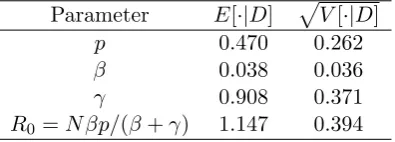
We applied the SIR epidemic model upon a Bernoulli random graph to the Gastroenteritis outbreak data given in example 2 above. We employed a vanilla ABC algorithm with U(0,1), Exp(0.2) and Exp(0.5) priors onp,β and γ, respectively, the same binning of time periods and distance metric as for the Markovian SIR model and= 10. We ran the algorithm to obtain 1000 accepted values from the (approximate) posterior distribution. This required 615596 simulations in R taking 930 seconds to complete with the resulting posterior estimates. The estimates for
p and R0 are similar to those reported in Britton and O’Neill (2002) with the estimates of β and γ being approximately two-thirds the values reported in Britton and O’Neill (2002). The discrepancy with Britton and O’Neill (2002) forβ andγ is due primarily to the way the removal times are modelled, in that, in Britton and O’Neill (2002) it is assumed that the removal times on day k all take place at the end of the day, whilst we assume that the removal times take place during the course of the day. The ABC-PMC algorithm performed poorly, with a very low acceptance rate. Hence, we have omitted its results. The reason is because the Normal proposal kernel (3) is a poor match to the “banana” shaped posterior dependence of p and β. A more sophisticated kernel or reparameterisation of the model might improve performance.
Parameter E[·|D] pV[·|D]
p 0.470 0.262
β 0.038 0.036
γ 0.908 0.371
[image:21.595.200.398.391.462.2]R0 =N βp/(β+γ) 1.147 0.394
Table 9: Approximate posterior moments for the parameters of the SIR model upon a Bernoulli random graph for the Gastroenteritis data
5
Conclusions
References
Bailey, N. T. (1975).The mathematical theory of infectious diseases and its applications. Charles Griffin & Company Ltd, 5a Crendon Street, High Wycombe, Bucks HP13 6LE.
Ball, F., Mollison, D., and Scalia-Tomba, G. (1997). Epidemics with two levels of mixing. The Annals of Applied Probability, 7(1):46–89.
Barber, S., Voss, J., and Webster, M. (2015). The rate of convergence for approximate Bayesian computation. Electronic Journal of Statistics, 9:80–105.
Beaumont, M., Zhang, W., and Balding, D. (2002). Approximate Bayesian Computation in Population Genetics. Genetics, 162(4):2025–2035.
Beaumont, M. A., Cornuet, J.-M., Marin, J.-M., and Robert, C. P. (2009). Adaptive approximate bayesian computation. Biometrika, 96(4):983–990.
Becker, N. (1989). Analysis of infectious disease data. Chapman & Hall/CRC.
Benenson, A. S. (1990). Control of communicable diseases in man. American Public Health Association.
Biau, G., C´erou, F., and Guyader, A. (2015). New insights into approximate Bayesian compu-tation. Annales de l’Institut Henri Poincar´e (B) Probabilit´es et Statistiques, 51(1):376–403.
Blum, M. G. B. (2010). Approximate Bayesian computation: A nonparametric perspective. Journal of the American Statistical Association, 105(491):1178–1187.
Blum, M. G. B., Nunes, M. A., Prangle, D., and A.Sisson, S. (2013). A comparative review of dimension reduction methods in approximate Bayesian computation. Statistical Science, 28:189–208.
Bornn, L., Pillai, N., Smith, A., and Woodard, D. (2016). The use of a single pseudo-sample in approximate Bayesian computation. arXiv preprint arXiv:1404.6298.
Boys, R. J. and Giles, P. R. (2007). Bayesian inference for stochastic epidemic models with time-inhomogeneous removal rates. Journal of Mathematical Biology, 55(2):223–247.
Britton, T. and O’Neill, P. D. (2002). Bayesian inference for stochastic epidemics in populations with random social structure. Scandinavian Journal of Statistics, 29(3):375–390.
Brooks-Pollock, E., Roberts, G. O., and Keeling, M. J. (2014). A dynamic model of bovine tuberculosis spread and control in great britain. Nature, 511(7508):228–231.
C´aceres, V. M., Kim, D. K., Bresee, J. S., Horan, J., Noel, J. S., Ando, T., Steed, C. J., Weems, J. J., Monroe, S. S., and Gibson, J. J. (1998). A viral gastroenteritis outbreak associated with person-to-person spread among hospital staff. Infection control and hospital epidemiology, pages 162–167.
Cauchemez, S., Carrat, F., Viboud, C., Valleron, A., and Boelle, P. (2004). A bayesian mcmc ap-proach to study transmission of influenza: application to household longitudinal data. Statis-tics in medicine, 23(22):3469–3487.
Cauchemez, S., Donnelly, C., Reed, C., Ghani, A., Fraser, C., Kent, C., Finelli, L., and Ferguson, N. (2009). Household transmission of 2009 pandemic influenza a (H1N1) virus in the united states. N Engl J Med, 361(27):2619–2627.
Chis-Ster, I. and Ferguson, N. (2007). Transmission parameters of the 2001 foot and mouth epidemic in great britain. PLoS One, 2(6):e502.
Clancy, D. and O’Neill, P. D. (2007). Exact bayesian inference and model selection for stochastic models of epidemics among a community of households. Scandinavian Journal of Statistics, 34(2):259–274.
Del Moral, P., Doucet, A., and Jasra, A. (2006). Sequential Monte Carlo samplers. Journal of the Royal Statistical Society: Series B (Statistical Methodology), 68(3):411–436.
Del Moral, P., Doucet, A., and Jasra, A. (2012). An adaptive sequential Monte Carlo method for approximate bayesian computation. Statistics and Computing, 22(5):1009–1020.
Demiris, N. and O’Neill, P. D. (2006). Computation of final outcome probabilities for the generalised stochastic epidemic. Statistics and Computing, 16(3):309–317.
Drovandi, C. C. and Pettitt, A. N. (2011). Estimation of parameters for macroparasite popula-tion evolupopula-tion using approximate Bayesian computapopula-tion. Biometrics, 67(1):225–233.
Eichner, M. and Dietz, K. (2003). Transmission potential of smallpox: estimates based on detailed data from an outbreak. American Journal of Epidemiology, 158(2):110–117.
Forrester, M., Pettitt, A., and Gibson, G. (2007). Bayesian inference of hospital-acquired infec-tious diseases and control measures given imperfect surveillance data. Biostatistics, 8(2):383.
Fox, J. P. and Hall, C. E. (1980). Viruses in families: surveillance of families as a key to epidemiology of virus infections. PSG Publishing Company Inc., 545 Great Road, Littleton, Massachusetts 01460, USA.
Gibson, G. J. and Renshaw, E. (1998). Estimating parameters in stochastic compartmental models using Markov Chain methods. IMA J. Math. Appl. Med. Biol., 15:19–40.
Gillespie, D. T. (1977). Exact stochastic simulation of coupled chemical reactions. The journal of physical chemistry, 81(25):2340–2361.
Hollingsworth, T. (2009). Controlling infectious disease outbreaks: Lessons from mathematical modelling. Journal of Public Health Policy, 30(3):328–341.
Jewell, C. P., Kypraios, T., Christley, R. M., and Roberts, G. O. (2009a). A novel approach to real-time risk prediction for emerging infectious diseases: a case study in avian influenza H5N1. Preventive veterinary medicine, 91(1):19–28.
Kypraios, T. (2007). Efficient Bayesian inference for partially observed stochastic epidemics and a new class of semi-parametric time series models. PhD thesis, Lancaster University.
Kypraios, T., O’Neill, P. D., Huang, S. S., Rifas-Shiman, S. L., and Cooper, B. S. (2010). As-sessing the role of undetected colonization and isolation precautions in reducing Methicillin-Resistant Staphylococcus aureus transmission in intensive care units. BMC Infectious Dis-eases, 10(1):29.
Lindvall, T. (1992). Lectures on the Coupling Method. Wiley, New York.
Longini, I. M., Koopman, J. S., Monto, A. S., and Fox, J. P. (1982). Estimating household and community transmission parameters for influenza. American Journal of Epidemiology, 115(5):736–751.
Marjoram, P., Molitor, J., Plagnol, V., and Tavar´e, S. (2003). Markov chain Monte Carlo without likelihoods. Proc. Natl Acad. Sci. USA, 100(26):15324.
McBryde, E., Gibson, G., Pettitt, A., Zhang, Y., Zhao, B., and McElwain, D. (2006). Bayesian modelling of an epidemic of severe acute respiratory syndrome. Bulletin of mathematical biology, 68(4):889–917.
McKinley, T., Cook, A. R., and Deardon, R. (2009). Inference in epidemic models without likelihoods. The International Journal of Biostatistics, 5(1).
Neal, P. (2012). Efficient likelihood-free bayesian computation for household epidemics.Statistics and Computing, 22(6):1239–1256.
Neal, P. and Roberts, G. (2005). A case study in non-centering for data augmentation: stochastic epidemics. Statistics and Computing, 15(4):315–327.
O’Neill, P. D., Balding, D. J., Becker, N. G., Eerola, M., and Mollison, D. (2000). Analyses of infectious disease data from household outbreaks by Markov Chain Monte Carlo methods. Journal of the Royal Statistical Society: Series C (Applied Statistics), 49(4):517–542.
O’Neill, P. D. and Roberts, G. O. (1999). Bayesian inference for partially observed stochastic epidemics. J. Roy. Statist. Soc. Ser. A, 162:121–129.
Prangle, D. (2015a). Adapting the ABC distance function. arXiv preprint arXiv:1507.00874.
Prangle, D. (2015b). Summary statistics in approximate Bayesian computation. arXiv preprint arXiv:1512.05633.
Pritchard, J., Seielstad, M., Perez-Lezaun, A., and Feldman, M. (1999). Population growth of hu-man Y chromosomes: a study of Y chromosome microsatellites.Mol. Biol. Evol., 16(12):1791– 1798.
Roberts, G. O., Papaspiliopoulos, O., and Sk¨old, M. (2003). Non-centered parameterisations for hierarchical models and data augmentation. In Bayesian Statistics 7: Proceedings of the Seventh Valencia International Meeting, page 307. Oxford University Press, USA.
Sisson, S. A. and Fan, Y. (2011). Likelihood-free MCMC. Handbook of Markov Chain Monte Carlo, pages 313–335.
Sisson, S. A., Fan, Y., and Tanaka, M. M. (2007). Sequential monte carlo without likelihoods. Proceedings of the National Academy of Sciences, 104(6):1760–1765.
Streftaris, G. and Gibson, G. (2004). Bayesian analysis of experimental epidemics of foot-and-mouth disease. Proceedings of the Royal Society B: Biological Sciences, 271(1544):1111.
Toni, T., Welch, D., Strelkowa, N., Ipsen, A., and Stumpf, M. (2009). Approximate Bayesian computation scheme for parameter inference and model selection in dynamical systems. J. R. Soc. Interface, 6:187–202.
A
PMC for partially coupled ABC algorithm
In this Section we outline how the partially coupled ABC-PMC algorithm can be implemented. The algorithm is based upon T PMC steps with the output from the final step used as an estimate from the posterior distribution. The generic algorithm below is given for obtaining samples from an approximation of π(θ|D), where the parameters θ can be partitioned into two groups φ and ϕ. For the parameters in φ we sample these and fix them for each simulation whereas for the parameters in ϕ we consider all possible parameter values. For the household epidemic example φ=λL (or φ= (λ, α) ifα is to be estimated) andϕ=λG. It will probably
Algorithm 10 Partially coupled ABC-PMC algorithm for household epidemics
Input: observed dataD, tolerances 1 and 2, parameters governingπ(λL) andπ(λG)
Output: Weighted samples from an approximateπ(λL, λG|D).
1. Initialisation:
(a) Set the distance metric for comparing summary statistics which in the case of the household epidemics are |PHk=1Pkl=0l(xlk −x∗lk)|, the total number of individuals
infected in the epidemic andPHk=1Pkl=0|xlk−x∗lk|, the difference in the configuration
of infectives within households.
(b) Set precisions 1 and 2 for accepting simulations.
2. Lett= 1.
3. Repeat the following steps untilN occurrences:
(a) Ift= 1 sample φ∗∗ fromπ(φ). Else, sample φ∗ from the previous population {φ(t−i)1}
with weights {w(ti−)1}. Perturb the particle to obtain φ∗∗ ∼ Kt(φ|φ∗), where Kt is
a pertubation kernel. Throughout we recommend a multivariate Gaussian kernel with covariance matrix twice the (weighted) empirical covariance matrix given by {(φ(ti−)1, w(t−i)1)}, see Beaumont et al. (2009).
(b) If π(φ∗∗) > 0, proceed with simulating from the partially coupled ABC algorithm using the parameters φ∗∗. Let C denote the set of ϕ parameters which result in an accepted simulation and letc=R
Cπ(ϕ)dϕ, the probability that a value ofϕsampled
from the prior will lie in C.
(c) Ifc >0, set φ(ti)=φ∗∗ and calculate the weight for particleφ(ti),
vt(i)=
1 ift= 1,
π(φ(ti))
PN j=1w
(j)
t−1Kt(φ (i)
t |φ
(j)
t−1)
ift >1,
with wt(i) = cv(ti). If t = T, set A(i) = C. That is, for the final step we record the set ofϕ for each accepted simulations. These are not required for taking forward the intemediary steps as theϕ parameters are effectively integrated out.
4. Normalise the weights to sum to 1. 5. Incrementt=t+ 1
6. Repeat Steps 3 and 4 until t=T.
The key difference to the ABC-PMC algorithm of Toni et al. (2009) is that we have to take account of the weight for the set of ϕ values in the coupled simulation which will result in a simulation being accepted. For the household epidemic moments ofλG can easily be estimated
from {(A(i), w(i)
T )} with a consistent estimate ofE[h(λG)|x∗] provided by N
X
i=1 v(Ti)
Z
A(i)
h(λG)π(λG)dλG
, N
X
i=1 vT(i)
Z
A(i)
π(λG)dλG.
h(·) is either polynomial or exponential which suffice for our needs for the household epidemic.
B
Parameter estimates for household epidemic data sets
Algorithm E[λG|D] p
V(λG|D) E[λL|D] p
V(λL|D) No. of Simulations Time
ABC 1.139 0.156 0.378 0.147 24062289 31597
cABC 1.144 0.164 0.371 0.148 235861 756
ABC-PMC 1.144 0.130 0.369 0.127 2802265 4046
[image:27.595.69.525.180.248.2]pcABC-PMC 1.154 0.168 0.366 0.139 174248 564
Table 10: Comparison of ABC algorithms for the Seattle influenza A data set with = (8,1) and intermediary thresholds = (20,3) and = (12,2) for the ABC-PMC algorithm.
Algorithm E[λG|D] p
V(λG|D) E[λL|D] p
V(λL|D) No. of Simulations Time
ABC 0.803 0.166 0.177 0.077 14905586 32952
cABC 0.802 0.165 0.174 0.080 232796 393
ABC-PMC 0.815 0.172 0.175 0.078 2967606 3362
[image:27.595.71.523.310.381.2]pcABC-PMC 0.801 0.172 0.176 0.078 151319 282
Table 11: Comparison of ABC algorithms for the Seattle influenza B data set with = (20,2) and intermediary thresholds = (50,5) and = (30,3) for the ABC-PMC algorithm.
Algorithm E[λG|D] p
V(λG|D) E[λL|D] p
V(λL|D) No. of Simulations Time
ABC 0.813 0.117 0.179 0.068 38126827 229535
pcABC 0.819 0.117 0.178 0.066 339775 1334
ABC-PMC 0.820 0.117 0.180 0.069 5077091 14196
pcABC-PMC 0.819 0.121 0.177 0.068 190664 906
Table 12: Comparison of ABC algorithms for the Tecumseh 1977-8 outbreak data set with= (50,4) and intermediary thresholds = (100,10) and= (70,6) for the ABC-PMC algorithm.
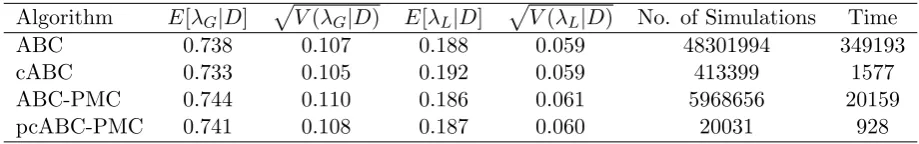
Algorithm E[λG|D] p
V(λG|D) E[λL|D] p
V(λL|D) No. of Simulations Time
ABC 0.738 0.107 0.188 0.059 48301994 349193
cABC 0.733 0.105 0.192 0.059 413399 1577
ABC-PMC 0.744 0.110 0.186 0.061 5968656 20159
pcABC-PMC 0.741 0.108 0.187 0.060 20031 928
[image:27.595.68.530.443.512.2] [image:27.595.69.529.573.645.2]