GNSS data filtering optimization for ionospheric observation

Optimization of the GNSS data filtering for

ionospheric observation

D’Angelo G.1_{, Spogli L.}2,3_{, Cesaroni C.}2_{, Sgrigna V.}1_{, Alfonsi L.}2_{, Aquino M.H.O.}4

1_{University of Rome “Roma Tre” (Italy), Via della Vasca Navale, 84, 00146 Rome, Italy}

2_{Istituto Nazionale di Geofisica e Vulcanologia (Italy), Via di Vigna Murata, 605, 00143 Rome, Italy}

3 _{SpacEarth Technology Srl (Italy), Via di Vigna Murata, 605, 00143 Rome, Italy}

4_{University of Nottingham (UK), Triumph Road, Nottingham NG7 2TU, United Kingdom}

Abstract

In the last years, the use of GNSS (Global Navigation Satellite Systems) data has been gradually increasing, for both scientific studies and technological applications. High-rate GNSS receivers, sampling the signal at 50 Hz, are commonly used to study the electron density irregularities within the ionosphere. The ionospheric irregularities may cause scintillations, which are rapid and random fluctuations of the phase and the amplitude of the received GNSS signals.

Usually, GNSS signals observed at an elevation angle lower than an arbitrary threshold (usually 15°, 20° or 30°) are filtered out from the sample, to remove the possible error sources due to the local environment where the receiver is deployed. Indeed, the signal scattered by environment (buildings, trees, etc.) could mimic ionospheric scintillation, because of the multiple scattering encountered by the signal passing through such structures.

Although widely adopted, the cut on the elevation angle has some downsides, as it may under or overestimate the actual impact of multipath due to local environment. Certainly, an incorrect selection of the field of view spanned by the GNSS antenna may lead to the misidentification of scintillation events at low elevation angles.

With the aim to tackle the non-ionospheric effects induced by multipath at ground, in this paper we introduce a filtering technique, termed SOLIDIFY (Standalone OutLiers IDentIfication Filtering analYsis technique), aiming at subtracting the multipath sources of non-ionospheric origin to optimise the field of view of a GNSS site. SOLIDIFY is a statistical filtering technique based on the signal quality parameters measured by the scintillation receivers. The technique is here applied and optimized on the data acquired by a scintillation receiver located at the Istituto Nazionale di Geofisica e Vulcanologia, in Rome. The results of the exercise show that, in the considered case of a noisy site under a quiet ionosphere, the SOLIDIFY optimization maximizes the quality, instead of the quantity, of the data.

1.

Introduction

Scintillation is most intense around ±15°/20° of magnetic latitude, and in auroral and polar cap regions of both hemispheres (see, e.g. Basu et al., 1988 and Kintner et al., 2009). In these ionospheric areas the electron density irregularities often form, because of the intense solar irradiation and of the solar wind-magnetosphere coupling (see, e.g. Kelley, 2009).

The investigation of fast small-scale irregularities causing radio scintillation can be carried out with special GNSS receivers sampling the satellite signal at high rate, such as 50 Hz (see, e.g. De Franceschi et al., 2006; Van Dierendonck, 2001). Although this sampling frequency is useful to investigate transient ionospheric effects, it cannot distinguish the scintillations caused by natural effects, such as ionospheric irregularities, from the multipath due to physical obstacles (buildings, trees, etc.), that may be present in the environment surrounding the receiver. Because of the multiple scattering encountered by the signal passing through such structures, the waves scattered by the environment could actually mimic ionospheric scintillation.

Currently, a fool-proof standard procedure able to remove short and long term effects due to environmental multipath has been not yet implemented, because no quantities, directly measured by the receiver, can separate ionospheric to environmental effects on the signal.

To overcome this issue, it is commonly adopted in the literature to filter out the observations below an arbitrary threshold on the elevation angle (αelev), typically 15°, 20° or 30°. Such cut is arbitrary, not physical, site independent and not standard. Moreover, this selection is often made at data acquisition level and not at data analysis level, leading to a definitive loss of scintillation data.

Therefore, in order to improve the quality of a GNSS site, it is necessary to identify and remove the outcome of the local environment that contaminates the scintillation measurements or, at least, to mitigate its effects, by wisely filtering the data sample.

Starting from the first step towards a new filtering technique done by Spogli et al. (2014), we testand refine the technique analysing the data collected by a GNSS receiver located at the headquarter of the Istituto Nazionale di Geofisica e Vulcanologia in Rome.

The site has been chosen because weakly affected by the ionosphere (on average quiet at mid-latitudes), but located into an urban context, where many sources of environmental multipath are present.

Hence, to optimize the previous filtering technique and to pinpoint the non ionospheric effects induced by multipath at ground, we implemented the SOLIDIFY (Standalone OutLiers IDentIfication Filtering analYsis) technique.

Thanks to an incisive discussion about outliers definition, to an extensive test of the signal quality parameters measured, and to a photographic and telemetric analysis of the Rome receiver, SOLIDIFY is able to give data-driven indications to efficiently remove those measurements affected by multipath. In agreement with the general theory statistical data analysis (see, e.g. Barnett and Lewis, 1995), we here consider as outliers those values of the signal quality parameters that are distant from the bulk of the distribution, i.e. values that lie in the tail(s) of the considered distributions.

SOLIDIFY is based upon the Ground Based Scintillation Climatology (GBSC) and upon a site characterisation technique inspirited by the work reported in Romano et al. (2013). The GBSC is a data analysis technique that was introduced to map the ionospheric irregularities producing scintillations over long-term periods and on selected areas (Spogli et al., 2009, Alfonsi et al., 2011).

This paper is organized as follows: section 2 introduces the data analysed in the study, section 3 describes the method adopted to implement SOLIDIFY, optimizing and testing different signal quality parameters by using the statistical filtering technique ; section 44 presents the results of the investigation; whereas, summary and concluding remarks are given in section 5.

2.

Data

The data here analysed have been acquired by a GISTM (GPS Ionospheric Scintillation and TEC Monitor) receiver located in Rome, Italy (receiver ID NSF01, geographic coordinates: 41°49’N, 12°30’E) from January 2013 to December 2014. The GISTM consists of a NovAtel GSV4004 dual frequency receiver owned by the University of Nottingham and hosted by Istituto Nazionale di Geofisica e Vulcanologia. GISTM samples at 50 Hz phase and amplitude and at 1 Hz code/carrier divergence for each satellite being tracked on L1. The receiver provides the following parameters measured on GPS signals:

 Phase scintillation index (σΦ), calculated over time intervals of 1, 3, 10, 30 and 60 seconds;

 TEC (Total Electron Content) and ROT (Rate of TEC change) every 15 seconds from L1 and L2;

 Code to Carrier Divergence (CC) and its standard deviation (CCSTDDEV), calculated over 60 seconds;

 Carrier to noise ratio (CN), every 60 seconds;

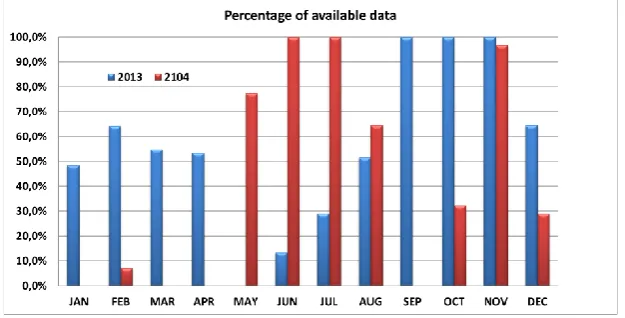
Since its deployment in 2012, the Rome GISTM receiver is set to acquire data only for observations made at αelev > 5°. In this paper, we have selected two years of data to propose a filtering method able to identify long-term effects on a large statistics. During the selected period, the data are available for 50% of the days. Despite this limitation in the data availability, we decided to use such sample because the receiver is located in a quiet ionospheric environment and characterized by the easiness in accessing the antenna for the photographic and telemetric analysis. The data availability is described in Figure 1 that presents the monthly percentage of available data in 2013 (blue histogram) and in 2014 (red histogram).

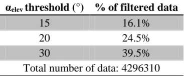
Figure 2 shows the percentage of the spatial data coverage considering the full dataset 2013-2014, obtained applying no threshold on the elevation angle (a) and with a threshold of 15° (b), 20° (c) and 30° (d). The coverage is projected to 350 km altitude, chosen as representative of the ionospheric F2-layer peak height. The comparison between the maps shows how the 15° cut-off significantly reduces the field of view spanned by GPS antenna. The percentages of filtered data, for different thresholds on the αelev, are summarized in Table 1.

Figure 2. Percentage of data coverage of the Rome receiver considering the full dataset 2013-2014, obtained applying no threshold on the elevation angle (a) and with a threshold of 15° (b), 20° (c) and 30° (d). Orange line represents the position of

the dip equator at ground. Maps describe the coverage projected at 350 km.

Table 1. Percentage of filtered data for different thresholds on the αelev

αelev threshold (°) % of filtered data

15 16.1%

20 24.5%

30 39.5%

Total number of data: 4296310

3.

Method

As the CCSTDDEV is suggested to be a good indicator of the multipath activity experienced by the receiver antenna (Van Dierendonck et al., 1993), Spogli et al. (2014) used the standard deviation of the CCSTDDEV (σCCSTDDEV, Standard Deviation of L1 Code/Carrier divergence) to perform an outliers analysis. That analysis was aimed at identifying those ray paths characterised by a large variability of CCSTDDEV. Such ray paths were tagged as affected by multipath and then removed for any further data analysis. For the details, the reader is referred to the original article.

To go beyond, in this work we introduce the following analyses:

1. consider additional signal quality parameters measured by the GISTM to tune the procedure;

2. consider not only the standard deviations (σ), but also the mean value (hereafter indicated in brackets < >) of such quality parameters;

3. optimize the outliers analysis by comparing different definition of outlier;

4. perform a photographic and telemetric analysis to consolidate what found by the data analysis.

 CCSTDDEV

 L1 C/N,

 CCSTDDEV/S4raw.

The aforementioned quantities are, respectively, the Standard Deviation of L1 Code/Carrier divergence, the L1 Carrier to Noise Ratio and a Multipath variable. The Multipath variable is defined according to Conker et al., 2002 (and references therein), where S4raw is the amplitude scintillation index not corrected for the thermal noise.

The bin size adopted to produce the GBSC maps is 5° in azimuth and 5° in elevation that results to be a good compromise between a fine fragmentation of the map and a meaningful statistics available in each bin. The identification of the bin in the GBSC maps, suspected to be affected by multipath, is based on the definition of outliers distribution. This distribution is derived by the general theory of statistical data analysis, without any a priori physical assumption (see, e.g., Barnett and Lewis, 1995).

As stated in point 2 in the above list, both mean and standard deviation are used to create corresponding histograms on which the outliers analysis is then applied. This exercise is repeated on all the analysed quantities.

According to the general theory of statistical data analysis (Barnett and Lewis, 1995), most values of the distribution are expected to fall in the inter-quartile range (IQR), that is the distance between the 1st _{and the} 3rd _{quartile. For single right tail distribution, the outliers are considered those lying above Q}

3+k·IQR, where Q3 is the 3rd quartile, while for single left distribution, the outliers are considered those lying above Q1

-k·IQR, where Q1 is the 1st quartile. k is the factor for determining the threshold for outliers.

In our analysis those bins corresponding to outliers values are identified and tagged as “suspected multipath”.

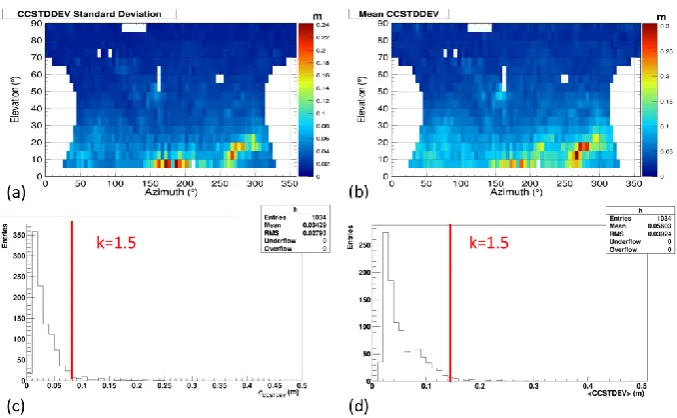
As an example, Figure 3a and Figure 3b show the GBSC maps of σCCSTDDEV and <CCSTDDEV> respectively, obtained considering the full dataset 2013-2014. White bins in the GBSC maps are in correspondence with ray paths not covered by the GPS constellation or they indicate that a meaningful statistics is not available in the specific bin. Figure 3c and Figure 3d show the corresponding histograms in which the red lines identify the cut-off obtained with k =1.5.

To compare the results of the outliers analysis on different histograms, maps like the one in Figure 4 are realised. For the remainder of the paper, such maps are called comparison maps. In Figure 4 we make a bin to bin comparison between σCCSTDDEV and <CCSTDDEV> filterings, respectively identified as histogram 1 and 2,adopting the following colour code:

 yellow indicates bins filtered out only with the outliers analysis of histogram 1;

 cyan indicates bins filtered out only with the outliers analysis of the histogram 2;

 red indicates bins filtered out with the outliers analysis of both histogram 1 and 2 (common results).

The exercise described in Figure 4 allows not only to improve the filtering presented by Spogli et al. (2014), but also to test different k values to extend the standard definition of outlier.

To optimize the outliers analysis we compare different definitions of outlier, i.e. different values of the k

parameter. Indeed, we test each signal quality parameter with different choice of k parameter, thus applying more severe or mild filters (see, e.g. Figure 3 c and d).

Figure 3. Maps of σCCSTDDEV (a) and <CCSTDDEV> (b) in azimuth vs. elevation from Rome GISTM receiver considering the full dataset 2013-2014. Corresponding distributions of the σCCSTDDEV (c) and <CCSTDDEV> (d). The red line indicates the

cut-off for k=1.5

Figure 4. Example of comparison between bins filtered out for 2 different histograms: yellow is for the bin filtered out by performing the outliers analysis on histogram 1 only, cyan is for histograms 2 only, while red identifies the bin commonly

identified.

4.

Results

environment, most of the bins identified as outliers are at lower elevation angles. Moreover, as expected from the definition of outlier, the number of tagged bins is larger for smaller values of k.

In each map of Figure 5, the comparison between mean and standard deviation of CCSTDDEV evidences that the bins commonly identified (in red) have a strong dependence on the k parameter. In particular, when k

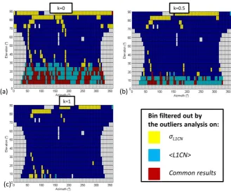
increases, the number of bins commonly identified as outliers decreases. Moreover, Figure 5 shows that when k value increases the bins filtered out by <CCSTDDEV> (cyan) are much less than those filtered out by σCCSTDDEV (yellow).

The comparison maps for k=1, 1.5 and 3 show that the common outliers highlight a sector in the azimuthal range between about 140° and 330°. For k=0.5 and k=1 it is highlighted also a region confined at around 50° of azimuth.

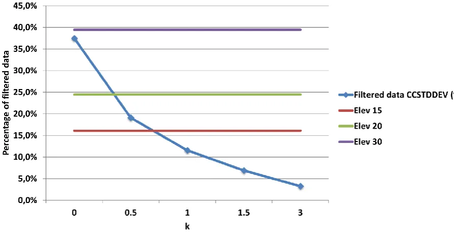
Figure 6 shows the percentages of CCSTDDEV filtered data as a function of the k parameter and for different thresholds on the elevation angle. As expected, when k value increases the percentage of filtered data decreases. The choice of k=0 results in a filter for outliers which is more severe than a thresholds on the elevation angle of 20°. That filtering is comparable to the threshold of 30°. Moreover, Figure 6 shows that by choosing k=1, 1.5 or 3 the percentage of filtered data is lower than by applying the 15° cut-off on the elevation angle.

We perform the same analysis on both Multipath and L1CN histograms to check if also these quality signal parameters are good indicators to catch the environmental multipath. Figure 7 shows the comparison maps of <Multipath> and σMultipath for the selected values of k. The maps show that the Multipath variable (CCSTDDEV/S4raw) is not suitable to identify long-term multipath effects at ground. The same figure shows also that most of the identified bins are at high elevation (up to 90°), where multiple scattering at ground do not take place.

A similar behaviour of L1CN at high and low elevation results from the comparison maps shown in Figure 8. Such maps do not include the values of k=1.5 and 3 because for these k values no <L1CN> outliers are identified. The maps evidence that the bins filtered by <L1CN> (cyan) are all found at low elevation, while those filtered by σL1CN (yellow) are found at high and low elevation.

Figure 9 and Figure 10 show the results of the photographic and telemetric analysis. These figures show how the Rome GNSS site is surrounded by buildings, trees, antennas, etc. that induce noise by the multipath point of view. Moreover, the azimuthal range between about 110° and 200° (Figure 9) is characterized by the presence of the roof of the INGV building. The roof effect is visible both in the comparison maps of CCSTDDEV (Figure 5) and Multipath (Figure 7), since from the k=3 map.

Figure 5. Comparison maps of <CCSTDDEV> and σCCSTDDEV for different values of k: k=0 (a), k=0.5 (b), k=1 (c), k=1.5 (d) and k=3 (e).

Figure 7. Comparison maps of <Multipath> and σMultipath for different values of k: k=0 (a), k=0.5 (b), k=1 (c), k=1.5 (d) and k=3 (e).

Figure 9. Photographic and telemetric analysis of the Rome station: azimuth sectors between 145° and 250°.

Figure 10. Photographic and telemetric analysis of the Rome station: azimuth sectors between 250° and 330°.

the enhancement of long term scintillation occurrence of both phase and amplitude is expected to be due primarily to multipath at ground.

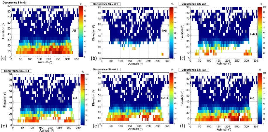
From both Figure 11 and Figure 12, k=0 is the most suitable outliers definition to realistically represent the ionosphere over Rome by removing the scintillation occurrence mimed by the multipath.

Figure 11. Percentage of occurrence of S4 above 0.1 obtained by considering all data (a) and data filtered by means of the <CCSTDDEV> plus σCCSTDDEV filtering (yellow+cyan+red bins in Figure 5) for k=0 (b), k=0.5 (c), k=1 (d), k=1.5 (e) and k=3

(f).

Figure 12. Percentage of occurrence of SigmaPhi above 0.1 obtained by considering all data (a) and data filtered by means of the <CCSTDDEV> plus σCCSTDDEV filtering (yellow+cyan+red bins in Figure 5) for k=0 (b), k=0.5 (c), k=1 (d), k=1.5 (e) and

5.

Summary and concluding remarks

This paper faces a delicate and crucial aspect of GNSS data analysis, i.e. the discrimination between ionospheric and environmental disturbances. In particular, this work is focused on the long term effects induced by the surrounding environment (trees, buildings, antennas, etc.), introducing an original approach proposed by Spogli et al. (2014) and here further optimized. The proposed optimization starts from the fundamental concept that a proper use of GNSS data has to be based on the maximization of the data quality. This comes with a downside: the possible reduction of usable data. The advantage is to dispose of a dataset able to provide the information needed to advance the current knowledge of the ionosphere.

The optimization leads to the following considerations:

1. The choices of k=1.5 and k=3 for CCSTDDEV (Figure 5), corresponding to the outliers identification proposed in the Spogli’s filtering, are too loose to characterize an environment known to be noisy by the multipath point of view. Thus, a tailored definition of outliers is crucial to efficiently remove the contribution of noisy ray-paths. In particular, the characterization of the Rome site, located under a quiet ionosphere but surrounded by many multipath sources, results in the choice of k=0 for the CCSTDDEV-based filtering (Figure 5a).

2. The choice of k=0 (point 1) is almost equal to apply a threshold on the elevation angle of 30° (Figure 6). Thus, in the Rome site case a blind cut-off of 20°, commonly adopted to remove the multipath, would not be efficient in providing a clean ionospheric information.

3. A comparative analysis of the filtering procedure based on CCSTDDEV, Multipath variable (CCSTDDEV/S4raw) and L1CN leads to the consolidation of the sole CCSTDDEV to be efficiently able in identifying multipath. However, by merging the filtering obtained by σCCSTDDEV and <L1CN> with k=0, it is possible to remove the bins saved by the CCSTDDEV-based filtering (point 1). In this way, we obtain a better performance in removing those bins affected by multipath at ground. This is shown in Figure 13, which reports the percentage of occurrence of S4>0.1 (a) and σΦ > 0.1 (b), applying the above mentioned merged filtering.

4. When possible, the photographic and telemetric analysis represents a fundamental tool to understand and characterize the site for a proper ionospheric monitoring. When conducted in the Rome site, the analysis leads to the fact that the scattering from the roof of the INGV headquarter is among the principal multipath sources besides tall buildings.

Thus, we propose a recipe, named SOLIDFY, to efficiently characterize the long-term multipath effects of a site, making it able to provide clean ionospheric measurements. SOLIDIFY is based on the following steps:

1. Acquire a statistically meaningful dataset from scintillation receivers. We propose to store at least 15-30 days of data.

2. Realise GBSC maps of CCSTDDEV and L1CN.

3. Perform the outliers analysis for different values of the k parameter. 4. Perform a telemetric and photographic analysis of the site.

5. Compare the results of point 3 and point 4 to efficiently choose the k parameter. 6. Remove those bins identified as outliers from the dataset at data analysis level.

Figure 13. Percentage of occurrence of S4>0.1 (a) and σΦ>0.1 (b) applying the merged filtering obtained by σCCSTDDEV and <L1CN> and using k=0 for the outliers definition.

Acknowledgements

XXXX

References

Alfonsi, L., Spogli, L., De Franceschi, G., Romano, V., Aquino, M., Dodson, A., Mitchell, C.N. Bipolar climatology of GPS ionospheric scintillation at solar minimum. Radio Sci. 46, RS0D05, http://dx.doi.org/10.1029/2010RS004571, 2011.

Barnett, V., Lewis, T., Outliers in Statistical Data. Wiley, 3rd Edition, 1995.

Basu, S., Mackenzie, E., Basu, S. Ionospheric constraints on VHF/UHF communication links during solar maximum and minimum periods. Radio Sci. 23 (3), 363–378, 1988.

Conker, R. S., M. B. El-Arini, K. Matsunaga, and K. Hoshinoo, Preliminary Analysis of the Effects of Ionospheric Scintillation on the MTSAT SatelliteBased Augmentation System (MSAS), Proceedings of IES2002, Alexandria, VA, May 2002.

Kelley, M. C. (2009). The Earth's Ionosphere: Plasma Physics & Electrodynamics (Vol. 96). Academic press.

Kintner, P. M., Humphreys, T., & Hinks, J. (2009). GNSS and ionospheric scintillation. Inside GNSS, 4(4), 22-30.

Prikryl P., Zhang Y., Ebihara Y., Ghoddousi-Fard R., Jayachandran P. T., Kinrade J., Mitchell C.N., Weatherwax A.T., Bust G., Cilliers P.J., Spogli L., Alfonsi L., Romano V., Ning B., Li G., Jarvis M.J., Danskin D.W., Spanswick E., Donovan E., Terkildsen M. (2013), An interhemispheric comparison of GPS phase scintillation with auroral emission observed at the South Pole and from the DMSP satellite. ANNALS OF GEOPHYSICS, 56, 2, R0216; doi:10.4401/ag-6227

Spogli, L., Alfonsi, L., De Franceschi, G., Romano, V., Aquino, M. H. O., & Dodson, A. (2009). Climatology of GPS ionospheric scintillations over high and mid-latitude European regions. Ann. Geophys, 27, 3429-3437.

Spogli, L., Romano, V., De Franceschi, G., Alfonsi, L., Plakidis, E., Cesaroni, C., Aquino M., Dodson A., Galera Monico J. F, Vani B.,(2014). A Filtering Method Developed to Improve GNSS Receiver Data Quality in the CALIBRA Project, Mitigation of Ionospheric Threats to GNSS: an Appraisal of the Scientific and Technological Outputs of the TRANSMIT Project, Dr. Riccardo Notarpietro (Ed.), ISBN: 978-953-51-1642-4, InTech, DOI: 10.5772/58778.

Van Dierendonck, A. J., Klobuchar, J., and Hua, Q.: Ionospheric scintillation monitoring using commercial single frequency C/A code receivers, in: ION GPS-93 Proceedings of the Sixth International Technical Meeting of the Satellite Division of the Institute of Navigation, Salt Lake City, USA, 22–24 September, 1333–1342, 1993.