Legitimising data driven models: exemplification of a new data driven mechanistic modelling framework

(1)

Hydrol. Earth Syst. Sci., 17, 2827–2843, 2013 www.hydrol-earth-syst-sci.net/17/2827/2013/ doi:10.5194/hess-17-2827-2013

EGU Journal Logos (RGB)

Advances in

Geosciences

Open Access

Natural Hazards

and Earth System

Sciences

Open Access

Annales

Geophysicae

Open Access

Nonlinear Processes

in Geophysics

Open Access

Atmospheric

Chemistry

and Physics

Open Access

Atmospheric

Chemistry

and Physics

Open Access Discussions

Atmospheric

Measurement

Techniques

Open Access

Atmospheric

Measurement

Techniques

Biogeosciences

Open Access Open Access

Biogeosciences

Discussions

Climate

of the Past

Climate

of the Past

Discussions

Earth System

Dynamics

Earth System

Dynamics

Discussions

Geoscientific

Instrumentation

Methods and

Data Systems

Open Access

_{Geoscientific}

Instrumentation

Methods and

Data Systems

Geoscientific

Model Development

Geoscientific

Model Development

Discussions

Hydrology and

Earth System

Sciences

Open Access

Hydrology and

Earth System

Sciences

Ocean Science

Discussions

Solid Earth

Discussions

The Cryosphere

Discussions

Natural Hazards

and Earth System

Sciences

Open Access

Discussions

Legitimising data-driven models: exemplification of a new

data-driven mechanistic modelling framework

N. J. Mount1, C. W. Dawson2, and R. J. Abrahart1

1_{School of Geography, University of Nottingham, Nottingham, NG7 2RD, UK}

2_{Department of Computer Science, Loughborough University, Loughborough, LE11 3TU, UK}

Correspondence to: N. J. Mount ([email protected])

Received: 11 December 2012 – Published in Hydrol. Earth Syst. Sci. Discuss.: 9 January 2013 Revised: 7 June 2013 – Accepted: 7 June 2013 – Published: 17 July 2013

Abstract. In this paper the difficult problem of how to

legit-imise data-driven hydrological models is addressed using an example of a simple artificial neural network modelling prob-lem. Many data-driven models in hydrology have been crit-icised for their black-box characteristics, which prohibit ad-equate understanding of their mechanistic behaviour and re-strict their wider heuristic value. In response, presented here is a new generic data-driven mechanistic modelling frame-work. The framework is significant because it incorporates an evaluation of the legitimacy of a data-driven model’s inter-nal modelling mechanism as a core element in the modelling process. The framework’s value is demonstrated by two sim-ple artificial neural network river forecasting scenarios. We develop a novel adaptation of first-order partial derivative, relative sensitivity analysis to enable each model’s mechanis-tic legitimacy to be evaluated within the framework. The re-sults demonstrate the limitations of standard, goodness-of-fit validation procedures by highlighting how the internal mech-anisms of complex models that produce the best fit scores can have lower mechanistic legitimacy than simpler counter-parts whose scores are only slightly inferior. Thus, our study directly tackles one of the key debates in data-driven, hydro-logical modelling: is it acceptable for our ends (i.e. model fit) to justify our means (i.e. the numerical basis by which that fit is achieved)?

1 Introduction

In this paper a new, data-driven mechanistic modelling framework (DDMMF) is presented as a response to the complex, long-standing problem of how to determine the

mechanistic legitimacy of a hydrological, data-driven model (DDM). The framework is inspired by earlier concepts em-bedded in the data-based mechanistic modelling (DBM) ap-proach of Young and Beven (1994), although it has a dis-tinctly different emphasis. In the DBM approach mecha-nisms found in data are used to identify appropriate models. In the DDMMF the mechanisms within the models them-selves are used to determine the most appropriate solutions. This represents a novel shift within data-driven modelling as it places an explanation of how data-driven models work at the centre of the model development and selection pro-cess – thus incorporating information that goes beyond out-puts and model fit. We here use the term “mechanistic” to refer to the interactions of the internal numerical mecha-nisms that control a model’s behaviour and the term “le-gitimacy” to refer to the degree of conformance between a model’s mechanistic behaviour and that sought by the mod-eller. The DDMMF is contextualised within the specific sub-set of artificial neural network (ANN) models, and is exem-plified via two simple neural network , hydrological forecast-ing problems. The paper presents an important new frame-work through which data-driven modellers in general, and ANN-based modellers in particular, can respond to concerns that their models lack the mechanistic legitimacy necessary if they are to deliver new insights that are widely accepted and trusted by hydrologists.

If the user of any model is to have confidence in it, the model development process must be seen to include ade-quate and explicit assessments of whether the system rep-resentation that is adopted, the inputs used, and the products that are delivered, are sufficient for the model’s intended pur-pose (Robinson, 1997). Where the purpur-pose is to develop a

(2)

2828 N. J. Mount et al.: Legitimising data-driven models

hydrological model that has value as a transferrable agent and can support new hydrological insights as well as enhanced prediction (i.e. Caswell’s, 1976, model duality), the model development and evaluation process should consider the le-gitimacy of its resultant modelling structures and their inter-nal mechanistic behaviours (e.g. Sargent, 2011). In the case of black-box hydrological models, achieving explicit legit-imisation of implicit modelling mechanisms is a major chal-lenge. Consequently, the use of black-box models is most commonly limited to catchment-specific, operational predic-tion tasks where there is usually no expectapredic-tion of model transferability. In such applications the model’s validity can be adequately assessed via the goodness-of-fit of its outputs (Klemes, 1986; Refsgaard and Knusden, 1996), but there is no formal requirement to legitimise the modelling mecha-nism by which the fit is obtained. This constrains the appli-cation of black-box models in hydrology which, like all mod-els, are limited in their use by their conceptual foundations.

In recent years the incorporation of increasingly complex machine-learning and artificial intelligence algorithms in hy-drological modelling applications has resulted in a prolif-eration of new DDMs in the literature (Solomatine et al., 2008). Some of these models do deliver explicit documen-tation of their internal mechanisms (e.g. see Mount et al., 2012, who explicitly document their gene expression pro-gramming and M5 model tree solutions). However, the nu-merical complexity of many models has meant that they are applied as black-box tools. These black-box DDMs are able to deliver predictive performance that is equal to or better than their physical or conceptual modelling counterparts (e.g. Shrestha and Nestmann, 2009). However, an important ques-tion remains about whether they can ever offer more than the optimisation of goodness-of-fit between inputs and outputs through the delivery of insights to hydrologists (Minns and Hall, 1996; Babovic, 2005; Abrahart et al., 2011). This ques-tion is particularly pertinent for ANN-based models, which represent the most widely used type of a black-box DDM in hydrology. Whilst we know that ANN-based models per-form well, we do not always understand why. Thus, the po-tential of ANN-based models as transferrable solutions, or as models that can deliver new insights into hydrological do-main knowledge redo-mains poorly demonstrated (Abrahart et al., 2012a). Indeed, DDMs in general, and ANN-based mod-els in particular, have been criticised as being little more than advanced curve-fitting tools with limited heuristic value (e.g. Abrahart et al., 2011). To those engaged in DDM and ANN-based modelling, this view can seem intuitively wrong. However, if such views are to be countered, researchers need to demonstrate much greater understanding about why and how such models deliver their results (c.f. Beven, 2002), and the minimum that must be delivered is a demonstration that DDMs possess two basic characteristics over and above their goodness-of-fit performance:

1. a logical and plausible structure (including input selection);

2. a legitimate mechanistic behaviour.

1.1 Evaluating the structure and behaviour of ANN models

The logic and plausibility of different ANN model structures has been a particular research focus in hydrology for more than a decade and significant advances have been made (e.g. Maier and Dandy, 2000, 2001). Research objectives have included the development of methods to improve input se-lection by input sensitivity analysis (e.g. Maier and Dandy, 1997; Sudheer, 2005) and by accounting for non-linearity and cross-correlation between potential inputs (e.g. partial mutual information (May et al., 2008). Similarly, informa-tion criteria have been used to identify the optimum number of hidden units by striking a balance between predictive per-formance and model complexity (e.g. Kingston et al., 2008). The examination of connection weights (Olden and Jackson, 2002) has also proven useful in the forecasting of hydrologi-cal variables in rivers (Kingston et al., 2003, 2006) by ensur-ing that the weights obtained durensur-ing model calibration make physical sense, even if this is at the expense of prediction accuracy (Kingston et al., 2005).

By contrast, advances towards delivering methods that can reveal and legitimise the internal, mechanistic behaviours of ANN models have been less forthcoming. Existing efforts have generally focussed on the ways in which an ANN parti-tions the input–output relaparti-tionship (Wilby et al., 2003; Jain et al., 2004; Sudheer and Jain 2004; See et al., 2008; Fernando and Shamseldin, 2009; Jain and Kumar, 2009). These studies have delivered useful hydrological insights into how different structural components of the ANN behave. However, they fall short of a comprehensive analysis of how the model’s overall response function behaves and whether the behaviour is legitimate. Because ANN models are usually treated as black-boxes, most researchers do not document their govern-ing equations as a means to support such an analysis. Even if the equations are delivered (e.g. Aytek et al., 2008; Abra-hart et al., 2009), their complexity prevents a straight forward behavioural interpretation.

(3)

N. J. Mount et al.: Legitimising data-driven models 2829

33

Figure 1. Conceptual elements in the legitimisation of data-driven hydrologic models. Dashed lines indicate the potential for the interaction of mechanistic and physical

legitimacy.

HYDROLOGIC DOMAIN KNOWLEDGE DATA-DRIVEN HYDROLOGIC

MODEL LEGITIMACY

Mechanistic Legitimacy

Physical Legitimacy

Legitimise Model Structure in terms of:

• Inputs; • Complexity; • Optimality; • Logic.

Legitimise Response Function Behaviour in

terms of:

• Magnitude; • Stability; • Continuity; • Coherency.

Fig. 1. Conceptual elements in the legitimisation of data-driven hy-drological models. Dashed lines indicate the potential for the inter-action of mechanistic and physical legitimacy.

verification (AIAA, 1998; Balci, 1998; Davis, 1992; Sargent, 1998, 2010), although by focussing on a model’s mechanics rather than its physical process representation, it avoids the difficult philosophical issues of “truth” that verification im-plies (see Oreskes et al., 1994 for an important discussion).

For this reason it is important to recognise that whilst mechanistic and physical legitimacy are strongly linked, they are not the same and should not be conflated (Fig. 1). The general sensibility of a model’s internal structure and be-haviour patterns does not necessarily equate to the extent to which they can be shown to map to the physical processes that are anticipated within a given catchment. Indeed, there is no reason to assume that adequate physical process knowl-edge will always be available to inform a given modelling context. Instead, mechanistic legitimacy may simply reflect the mechanical behaviour of the model’s response function: i.e. its magnitude, stability, continuity and coherency. Mech-anistic legitimacy per se can be an important concept for sup-porting model selection above and beyond goodness-of-fit metrics. For example, an ANN response function that dis-plays low continuity in its mechanistic behaviour is likely to be indicative of over-fitting. This is an important mechanis-tic characterismechanis-tic of a model that cannot be easily detected via goodness-of-fit, and that reduces the legitimacy of the model. It is also a characteristic that does not have any direct physical interpretation.

2 The data-driven, mechanistic modelling framework

The DBM approach (Young and Beven, 1994) for hydrolog-ical model development is of particular relevance as it offers a recognised means by which the legitimacy of a

hydrolog-34

Figure 2. Reordering of the DBM framework to generate the DDMMF. Grey dashed lines indicate where conceptual steps contained within the DBM approach are

[image:3.595.313.544.59.353.2]

incorporated into the DDMMF approach.

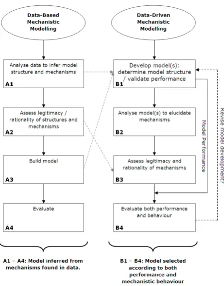
Fig. 2. Reordering of the DBM framework to generate the DDMMF. Grey dashed lines indicate where conceptual steps contained within the DBM approach are incorporated into the DDMMF approach.

ical model’s mechanistic behaviours can be evaluated in the absence of explicit, a priori knowledge about its governing equations. In the DBM approach, a model’s mechanistic be-haviour is assessed using a formal process of statistical infer-ence through which the required modelling mechanisms and behaviours are identified prior to building the model, and in-terpreted according to the extent to which they conform to the nature of the system under study (Young et al., 2004) (Fig. 2, A1–A4). The model is then accepted, or rejected, on the basis of its conformance.

The direct translation of the DBM approach to any DDM, including ANN-based examples, is prevented due to the means by which the DDM mechanisms are learnt directly from the data. This limits the a priori application of statisti-cal inference from which a mechanistic interpretation could perhaps be made. The DBM process can, however, be re-ordered to address this issue and better reflect the generic DDM process. Firstly, the analysis of data as a means of informing model structure is conflated with model build-ing to ensure that the structural and performance consider-ations within the DDM model development process are ad-equately represented (Fig. 2, B1). Secondly, analysis and legitimacy assessment of the resultant DDM’s mechanisms follows the normal model development activities (Fig. 2, B2–B3). Finally, model evaluation incorporates both model

[image:3.595.50.286.64.253.2]

(4)

performance (i.e. its validity as assessed by fit metrics) and the legitimacy of its behaviour to determine whether further model development work is required.

The result is a new, DDMMF that includes a specific re-quirement for mechanistic analysis and assessment to follow standard model development activities. This basic framework is generic and should be widely applicable across a range of data-driven modelling approaches, as well as being of partic-ular value for ANN-based models. It is more loosely defined than its DBM counterpart and need not necessarily be con-strained to a demonstration of adequate representation of a natural system by a model, which is a key feature of the DBM approaches. Indeed, it may also be used as a tool to direct broader mechanistic investigations, including the complexity and functionality of the internal workings of a model, and the extent to which these can be justified by the modelling task.

2.1 Enabling the DDMMF for ANN models: revealing mechanistic behaviour.

Enabling the DDMMF is reliant on the availability of tech-niques by which a model’s mechanistic behaviour (i.e. its magnitude, stability, continuity and coherency) can be legit-imised (Fig. 2, Box B2). Whilst these are not generally well developed for DDMs, conceptual and physically based mod-ellers have made extensive use of relative parameter sensi-tivity analysis (Hamby, 1994) to elucidate the mechanistic behaviour of their models (Howes and Anderson, 1988) and strengthen their validation (e.g. Kleijnen, 1995; Kleijnen and Sargent, 2000; Fraedrich and Goldberg, 2000; Smith et al., 2008; Mishra, 2009). Critically, it has been shown to be an important means by which model validation can be extended beyond fit, to include deeper insights into the legitimacy of a model’s mechanistic behaviours (e.g. Sun et al., 2009).

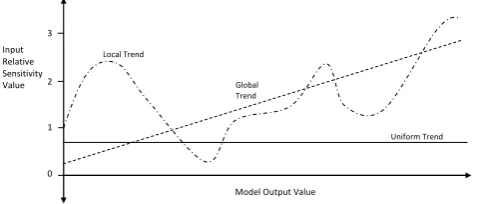
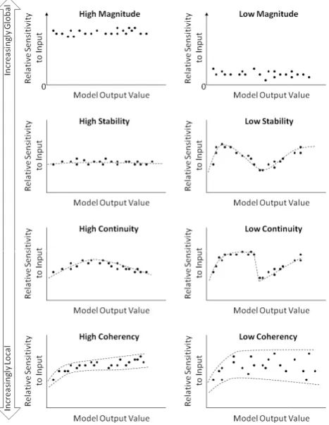
The pattern of variation in relative sensitivity values ex-ists on a continuum between global and local trends (Fig. 3). Where low variation in relative sensitivity occurs across the output range, the dominance of global mechanistic be-haviours can be inferred. Where higher levels of variation oc-cur, more complex, locally dominant mechanistic behaviours may be inferred. Taking this basic idea a step further, relative parameter sensitivity patterns can be characterised accord-ing to their magnitude, stability, continuity and coherency (Fig. 4). The magnitude of a model’s sensitivity to its inputs characterises the relative extent to which each model forecast is sensitive to variation in each of its inputs. It can therefore reveal the relative importance of each input as a driver of the model output at any given point in the forecast range. The stability of the input sensitivity characterises the consistency with which each input influences the model output across dif-ferent forecast ranges. Invariance in an input’s relative sensi-tivity across the entire range (the most stable case) indicates that it is being used as a constant multiplier by the model’s internal mechanism. Lower levels of stability will indicate in-creasingly non-linear influences. The existence of local

dis-35

Figure 3. Examples of relative sensitivity trends on the global-local continuum. The relative sensitivity value computed for any given point in the model output range indicates its response ratio magnitude at that point (i.e. the relative rates of change in the input and output). Trends can then be fitted through the scatter of points generated

by computing the relative sensitivity for any set of input / output records. Uniform trends are indicative of models where the local input / output response ratios do not vary

across the range of model outputs. Global trends are indicative of input / output response ratios that vary in a consistent manner. Local trends exhibit high variability in

their input / output response ratios.

Input Relative Sensitivity Value 2

1

0

Model Output Value

Uniform Trend Global

Trend Local Trend

3

Fig. 3. Examples of relative sensitivity trends on the global–local continuum. The relative sensitivity value computed for any given point in the model output range indicates its response ratio mag-nitude at that point (i.e. the relative rates of change in the input and output). Trends can then be fitted through the scatter of points generated by computing the relative sensitivity for any set of in-put/output records. Uniform trends are indicative of models where the local input/output response ratios do not vary across the range of model outputs. Global trends are indicative of input/output re-sponse ratios that vary in a consistent manner. Local trends exhibit high variability in their input/output response ratios.

continuities in a model’s sensitivity to an input indicates the existence of thresholds in the model’s mechanisms that may result in distinctly different internal mechanistic behaviour at neighbouring locations in the forecast range. Coherency re-flects the extent to which a model’s sensitivity to its inputs varies from point to point. Low coherence is indicative of a model that applies a distinctly different modelling mecha-nism to each local data point and is a means by which data overfitting may be detected.

Although methods for computing relative parameter sen-sitivities are not yet available for all DDMs, recent work has focussed on how it may be achieved for ANN models (Yeung et al., 2010). This has provided new opportunities for explor-ing their mechanistic behaviour within the DDMMF. Impor-tantly, computational techniques for determining first-order partial derivatives of certain ANNs have been available for some time. One such technique, outlined by Hashem (1992), involves the application of a simple backward chaining par-tial differentiation rule. His general rule is adapted in Eq. (1) for ANNs with sigmoid activation functions, a single hidden layer,i input units,nhidden units and one output unit (O), so that the partial derivative of the network’s output can be calculated with respect to each of its inputs (I):

∂O ∂Ii =

n X

j=1

wijwj Ohj(1−hj)O(1−O), (1)

where,wij is the weight from input unitito hidden unitj; wj O is the weight from hidden unitj to the output unitO; hj is the output of hidden unitj; andO is the output from the network.

[image:4.595.309.548.65.167.2]

(5)

Figure 4. Characteristic patterns of

arrow on the left indicates the relative focus of each sensitivity characteristics on a range

36

Characteristic patterns of relative sensitivity. The continuum

arrow on the left indicates the relative focus of each sensitivity characteristics on a range between global and local.

[image:5.595.52.286.66.368.2]

sensitivity. The continuum indicated by the arrow on the left indicates the relative focus of each sensitivity characteristics on a range

Fig. 4. Characteristic patterns of relative sensitivity. The continuum indicated by the arrow on the left indicates the relative focus of each sensitivity characteristic on a range between global and local.

Sensitivity values computed in an absolute form (Eq. 1) are inappropriate for the comparison of sensitivity values be-cause their values vary according to the magnitude of the parameters in the equation (McCuen, 1973). Relative sen-sitivity values (Eq. 2) are invariant to the magnitude of the model inputs and thus provide a valid means for comparing sensitivity values.

Rs= ∂O/O

∂Ii/Ii = ∂O ∂Ii ·

Ii

O (2)

The relative sensitivity of each input is thus calculated as ∂O

∂Ii ·Ii

O =

n X

j=1

wijwj Ohj(1−hj)O(1−O)· Ii O

=(1−O)Ii n X

j=1

wijwj Ohj(1−hj). (3)

It should be noted that the relative sensitivity values associ-ated with a model will vary continuously across the input– output space and each input will have a unique pattern of rel-ative sensitivity. A model’s relrel-ative sensitivity should, there-fore, be examined by comparison of the characteristic rela-tive sensitivity patterns associated with the different model

inputs, and should not be assessed via the comparison of individual, global statistics.

3 Exemplifying the DDMMF: the simple case of ANN-based river forecasting.

To exemplify the use of our DDMMF we here take the rel-atively simple case of an artificial neural network river fore-caster (NNRF) as a simple starting point. The basic jobs of a river forecasting model are defined by NOAA (2011) as: “. . . to estimate the amount of runoff a rain event will gen-erate, to compute routing, how the water will move down-stream from one point to the next, and to predict the flow of water at a given forecast point through the forecast period.”

These models have become one of the most popular ap-plication areas for data-driven modelling in hydrology over recent years (Abrahart et al., 2012a). In common with estab-lished, statistical river forecasting approaches (e.g. Hipel et al., 1977), each NNRF is a simple, short-step-ahead hydro-logical forecasting model whose predictions are derived from a core set of lagged, autoregressive model inputs recorded for the point at which the prediction is required (e.g. Fi-rat, 2008), and/or gauged locations upstream (Imrie et al., 2000). These inputs may be augmented by a range of rele-vant, lagged hydrometeorological variables that act to further refine the model output (e.g. Anctil et al., 2004); resulting in a black-box model that generally performs well (e.g. Abra-hart and See, 2007), but that lacks an explicit documentation of its internal mechanisms. The common objective of previ-ous studies (e.g. Coulibaly et al., 2000; Huang et al., 2004; Kis¸i and Cigizoglu, 2007; Kis¸i, 2008) has been to demon-strate that improved river forecasting can be achieved using NNRFs. NNRFs have the potential to deliver river forecasts with reduced error and recent work (de Vos, 2013) has high-lighted how the application of more complex, echo state net-works within NNRF studies may extend the reliable forecast horizon. By contrast, our objective is to exemplify how the application of input sensitivity analysis, delivered within the DDMMF, provides an important new means by which NNRF modellers can identify the most legitimate model mecha-nisms occurring inside a set of candidate models. Indeed, we restrict our modelling to only simple examples that use temporally lagged discharge; accepting that alternative in-put configurations may possibly be able to deliver superior models with an even higher degree of fit.

Our example ANN models incorporate simple structures and internal mechanistic behaviours that can be very eas-ily presented and understood. Indeed, the fact that data-driven modellers do not often seek to legitimise their mod-elling mechanisms suggests that the key concepts and argu-ments presented in Sect. 1 are not fully embedded in prac-tice, and so the clearest and most straight-forward examples are required to exemplify them. Similarly, by using example models that do not lend themselves to a detailed, physical

(6)

37

Figure 5. River Ouse catchment in North Yorkshire, UK

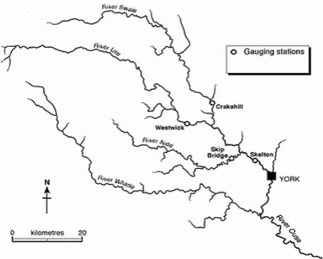
Fig. 5. River Ouse catchment in North Yorkshire, UK.

interpretation (autoregressive river forecasting models do not have any real physical basis and so cannot and should not be interpreted in these terms), we ensure that the legitimisation of mechanistic behaviour through the DDMMF remains the salient focus of the paper.

3.1 Study area, datasets and modelling scenarios

Two differently configured NNRFs are developed for the River Ouse at Skelton, Yorkshire, UK. The first NNRF (Sce-nario A) represents the most simplistic, autoregressive river forecasting case, in which at-a-gauge discharge is forecast from lagged discharge inputs recorded at the same loca-tion. The second, more complex, NNRF (Scenario B) pre-dicts at-a-gauge discharge from a set of three lagged dis-charge inputs recorded at gauges located in tributary rivers immediately upstream.

The catchment upstream of the Skelton gauge (Fig. 5) covers an area of 3315 km2with a maximum drainage path length of 149.96 km, and an annual rainfall of 900 mm. The catchment contains mainly rural land uses with<2 % ur-ban land cover. It exhibits significant areas of steep, moun-tainous uplands that extend over 12 % of the catchment, and includes three sub-catchments, comprising the rivers Swale, Ure and Nidd. Each of these tributaries is gauged in its low-land reaches, upstream of its confluence with the Ouse. De-tails of these gauges and contributing catchments are pro-vided in Table 1.

All NNRFs were developed using daily mean discharge records, downloaded from the Centre for Ecology and Hy-drology National River Flow Archive (www.ceh.ac.uk/data/ nrfa). The data extend over a period of 30 yr, from 1 Jan-uary 1980 to 31 December 2010 (Fig. 6). Several short gaps exist in the observed records at irregular periods across the different stations; necessitating approximately 8 % of the

Figure 6. Hydrographs for the four gauging stations showing data partitioning.

38

Hydrographs for the four gauging stations showing data partitioning. Hydrographs for the four gauging stations showing data partitioning. Fig. 6. Hydrographs for the four gauging stations showing data par-titioning.

30 yr record to be omitted due to missing records at one or more gauges.

The data were partitioned so that the first 75 % of the available record (7762 data points) was used for model calibration, leaving 25 % (2588 data points) for use in cross-validation (which we hereafter term “validation”) and model selection. This split places the three unusually high-magnitude flood peaks observed at Skelton (identified by the arrows in Fig. 6) in the calibration data. This is impor-tant in the context of our study, as it ensures that the in-ternal mechanisms of the calibrated models have been de-veloped to accommodate the largest observed floods in our dataset. Therefore, any mechanistic interpretation is informa-tive across the full forecast range for each model. Nonethe-less, we also recognise that the simplicity of this splitting procedure contrasts with more complex approaches that have been used by other ANN modellers (e.g. Snee, 1977; Bax-ter et al., 2000; Wu et al., 2012) to deliver improved valida-tion consistency (LeBaron and Weigend, 1998) by ensuring representative sub-setting procedures. Therefore, exceedance curves for the calibration and validation data (Fig. 7) were checked to ensure high conformance in the discharge proba-bility distributions for calibration and validation data subsets at all gauges.

3.2 Input selection and model development

[image:6.595.50.285.61.249.2] [image:6.595.306.547.62.291.2]

(7)

[image:7.595.129.467.82.395.2]

Table 1. Description of the River Ouse catchment and its primary sub-catchments.

Gauge ID Catchment Physiography Land Cover

Ouse at Skelton

27009 Area 3315 km2

Max Elevation 714 m AOD* Min Elevation 4.6 m AOD Majority high to moderate permeability bedrock

Woodland 7 %

Arable/Horticultural 31 % Grassland 44 %

Mountain/Heath/Bog 12 % Urban 2 %

Other 4 %

Swale at Crakehill

27071 Area 1363 km2

Max Elevation 714.3 m AOD Min Elevation 12 m AOD Majority high to moderate permeability bedrock

Woodland 6 %

Other 5 %

Nidd at Skip Bridge

27062 Area 516 km2

Max Elevation 702.6 m AOD Min Elevation 8.2 m AOD Majority high to moderate permeability bedrock

Woodland 8 %

Other 5 %

Ure at Westwick

27007 Area 915 km2

Max Elevation 710.0 m AOD Min Elevation 14.2 m AOD Majority moderate permeability bedrock

Woodland 8 %

Other 2 %

* Above Ordnance Datum.

Figure 7. Exceedence probability plots for the four gauging stations.

39

Exceedence probability plots for the four gauging stations. Exceedence probability plots for the four gauging stations.

Fig. 7. Exceedance probability plots for the four gauging stations.

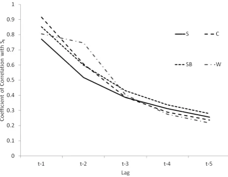
discharge record for Skelton, with no pre-processing having been applied. Three antecedent predictors were used, such lags having the strongest correlation with observed flow at Skelton at timet (Fig. 8) over the entire 30 yr record. Sce-nario B predicts St on the basis of antecedent discharges recorded for the three tributary gauges at Crakehill (C), Skip Bridge (SB) and Westwick (W). The strength of the correla-tion between each tributary gauge and Skelton over a range

Figure 8.

40

Lag analysis for the four gauging stations.Lag analysis for the four gauging stations.

Fig. 8. Lag analysis for the four gauging stations.

of lags was used to determine the lag time for each tribu-tary that represented the strongest predictor of St. The three inputs to Scenario B are thus Ct−1; SBt−1; and Wt−1.

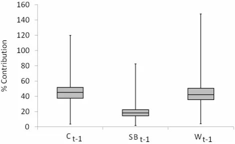
The proportion of the discharge at St that is accounted for by discharge at Ct−1, SBt−1 and Wt−1 is summarised as a box plot in Fig. 9. For each station, each lagged daily

[image:7.595.311.542.424.603.2] [image:7.595.49.285.428.578.2]

(8)

41

Figure 9. Proportional contributions of lagged upstream inputs to discharge forecast at Skelton.

Fig. 9. Proportional contributions of lagged upstream inputs to dis-charge forecast at Skelton.

mean discharge value was expressed as a proportion of the daily mean discharge at Skelton; resulting in a distribution of its upstream contribution. The median, inter-quartile range and max/min values of these distributions were used to pro-duce Fig. 9. The plot shows that, summarised over the whole record, lagged discharge at Crakehill and Westwick accounts for a similar proportion of the instantaneous discharge at Skelton, with comparable median values (∼40 %) and inter-quartile ranges. Skip Bridge is proportionally less impor-tant with a median value of 18 %. This highlights its relative weakness as a physical driver of St, which is in contrast to its relative strength as a statistical driver (i.e. it has the second highest correlation coefficient at t−1). It should be noted that, due to timing effects and the use of summary, daily mean data, the maximum proportional contributions values in Fig. 9 exceed 100 %.

[image:8.595.49.285.63.207.2]

In order to reflect the lack of consensus surrounding NNRF parameterisation, and the empirical process that un-derpins model selection in the majority of previous stud-ies, four candidate single-hidden-unit ANNs were developed for Scenarios A and B. Each candidate was structurally dis-tinct, incorporating either 2, 3, 4 or 5 hidden units. In this way, a range of alternative candidate models of varying com-plexity were developed in each NNRF scenario for subse-quent mechanistic comparison. All candidate model weights were calibrated using the back propagation of error learn-ing algorithm (Rumelhart et al., 1986). Learnlearn-ing rate was fixed at 0.1. Momentum was set at 0.9. The objective func-tion was root mean squared error (RMSE). Each candidate model was trained for 20 000 iterations on the first 75 % of the data record, and cross-validated against the remain-ing 25 % at 100 epoch intervals. Final model selection was made according to the lowest RMSE value obtained. The pre-ferred number of epochs for each hidden unit configuration for the different scenarios is shown in Table 2, with the rel-ative strength of the autoregressive relationship in Scenario A reflected in its lower number of training epochs. Similarly, the relative simplicity of the ANN configurations comprising

Table 2. Epochs for preferred NNRFs based on validation data.

Model Scenario Hidden Units

2 3 4 5

A 700 1100 3000 800

B 1000 7000 20 000 20 000

fewer hidden units is reflected in their generally lower num-ber of training epochs. Following the arguments in Abrahart and See (2007), and Mount and Abrahart (2011a), we also include two simple multiple linear regression (MLR) bench-marks. These are included to make clear the difficulty of the modelling task and the non-linearity of any required solution. Their equations are

Scenario A:St=6.014+1.12∗St−1+0.455∗St−2

+0.216∗St−3, (4)

Scenario B:St=5.715+0.424∗Ct−1+1.556∗SBt−1

+1.055∗Wt−1. (5)

3.3 NNRF relative sensitivity analysis

Equation (3) presents a generic computational method for de-riving first-order partial derivatives of an ANN-based model, from which mechanistic behaviours can be explored. How-ever, the use of these derivatives as the basis for develop-ing a parameter sensitivity analysis of NNRFs is complicated by the strong temporal dependencies that exist between the lagged model inputs. Standard, local-scale sensitivity analy-sis techniques (e.g. Turanayi and Rabitz, 2000; Spruill et al., 2000; Holvoet et al., 2005; Hill and Tiedeman, 2007) require the establishment of a representative base case (Krieger et al., 1977) for all inputs. This is usually defined according to their mean or median values on the assumption that all inputs are independent of one another. However, in NNRF modelling this assumption is not valid and the identification of a repre-sentative base case is very difficult (Abrahart et al., 2012b). Moreover, local scale analyses can only provide mechanis-tic insights for the specific location in the input hyperspace to which the base case corresponds, and it should not be as-sumed that mechanistic insights can be generalised beyond it (Helton, 1993).

[image:8.595.322.530.83.145.2]

(9)

[image:9.595.53.280.94.179.2]

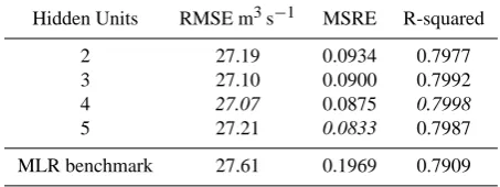
Table 3. Calibration performance of candidate models for Scenario A. Best performing ANN models for each metric are in italic.

Hidden Units RMSE m3s−1 MSRE R-squared

2 27.19 0.0934 0.7977

3 27.10 0.0900 0.7992

4 27.07 0.0875 0.7998

5 27.21 0.0833 0.7987

MLR benchmark 27.61 0.1969 0.7909

appropriate sampling strategy problematic. In addition, the summary, lumped indices output by global and regional tech-niques mask the detailed, local patterns of input–output sen-sitivity that must be understood in order to fully characterise a model’s mechanistic behaviour.

One solution for overcoming these difficulties is to adopt a brute-force approach in which relative first-order partial derivatives for all model inputs are computed separately for every data point in a given time series, using the specific in-put values recorded at each point as a datum-specific base case. In this way, a “global–local” parameter sensitivity anal-ysis is developed in which local-scale input sensitivity analy-sis is performed across the global set of available data points. Issues associated with temporal dependence in river forecast-ing data are overcome because every datum in the analy-sis effectively becomes its own, specific base case. NNRF mechanisms can then be characterised and interpreted across the full forecast range by plotting the relative sensitivity of each input (y axis) against the forecast values delivered by the model (x axis), and interpreting the patterns that can be observed in the plots (Fig. 4).

4 Scenario A: performance, mechanistic interpretation and model choice

4.1 Candidate model fit

[image:9.595.312.544.94.178.2]

The calibration and validation performance of each candidate NNRF, driven by autoregressive inputs, are presented in Ta-bles 3 and 4. A wide range of metrics has been proposed for assessing hydrological model performance (Dawson et al., 2007, 2010), along with a range of mechanisms for their in-tegration (e.g. Dawson et al., 2012). Nonetheless, consensus has still to be achieved on the metrics that should be used in assessing NNRF performance. Here we restrict our metrics to three simple and widely used examples that cover key aspects of model fit. This restriction is justified on the basis that the mechanistic exploration delivered by the DDMMF reduces the overall reliance on metric-based assessment and the im-portance of arguments that surround the subtleties of met-ric choice in model assessment. Pearson’s product–moment correlation coefficient, squared (R squared), is included as

Table 4. Validation performance of candidate models for Scenario A. Best performing ANN models for each metric are in italic.

Hidden Units RMSE m3s−1 MSRE R-squared

2 26.25 0.0825 0.8034

3 26.26 0.0809 0.8035

4 26.28 0.0794 0.8034

5 26.32 0.0752 0.8042

MLR benchmark 21.69 0.1151 0.8657

a general, dimensionless measure of model fit that indicates the proportion of overall variance in our data that is explained by each candidate model. RMSE is included because it is a metric that is disproportionately influenced by the extent to which each candidate model forecasts high-magnitude dis-charges. In contrast, the relative metric mean squared rela-tive error (MSRE) is included because its scores emphasise the extent to which low-magnitude discharges are correctly forecast by the candidates. The reported scores were com-puted using HydroTest (www.hydrotest.org.uk): an open ac-cess website that performs the required calculations in a stan-dardised manner (Dawson et al., 2007, 2010). The formula for each metric used can be found in Dawson et al. (2007).

The metric scores highlight almost identical levels of per-formance across the candidates, irrespective of the metric against which fit is assessed, or whether the fit is assessed relative to the calibration or validation data. Metric scores for the validation data are slightly better than those for the calibration data in all metrics, with the greatest differences observed in RMSE scores. This reflects the fact that the three highest magnitude floods are within the calibration data and, in common with most other autoregressive river forecasting models, there is a general underestimation of flood peaks. These two aspects combine to produce the observed improve-ment in RMSE in the validation data. Importantly, the MLR benchmark performs well, with RMSE and R-squared scores that are comparable with the NNRF candidates for the cal-ibration data and better for the validation data. This serves to highlight the slight characteristic differences between the calibration and validation data and the tendency of an ANN solution to optimise its fit to the calibration dataset. This ten-dency is avoided in simple MLR models due to the constraint of the model form which can lead to a higher level of gen-eralisation capability. As a result, the MLR performs better than the ANN solution when evaluated against the validation data, despite its poorer relative performance in calibration. It also serves to reinforce the argument that many simple au-toregressive river forecasting tasks are of a near-linear nature. Despite there being no clear winner on the basis of metrics alone, the 5-hidden-unit model does achieve the best NNRF candidate metric scores in three out of six cases.

(10)

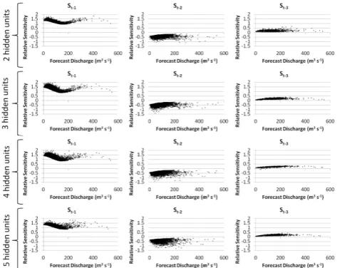
Figure 10. Global-local relative sensitivity plots for all candidate models in Scenario A

42

local relative sensitivity plots for all candidate models in Scenario A calibration data.

local relative sensitivity plots for all candidate models in Scenario A: Fig. 10. Global–local relative sensitivity plots for all candidate mod-els in Scenario A: calibration data.

4.2 Candidate model mechanisms

For each of the four candidate solutions, relative first-order partial derivatives were computed according to the global– local approach outlined in Sect. 3.3. Equation (3) was used to compute local first-order partial derivatives for the entire record (i.e. all 10 350 data points). Values ofwij,wj O, and hj were determined for each forecast, according to its spe-cific input value set at each point. These values are sepa-rated into their respective calibration/cross-validation parti-tions and plotted against their respective forecasted discharge values in Figs. 10 and 11.

Figures 10 and 11 highlight the fact that, mechanistically, all four candidate models behave in very similar ways and this behaviour is consistent across the calibration and val-idation data partitions. The similarity of relative sensitivity patterns in the calibration and validation data subsets is to be expected given the large data record being modelled and the similarity of each subset’s hydrological characteristics as demonstrated in Fig. 7. In all cases, the relative sensitivity of the model forecast to variation in St−1is substantially greater than to either St−2or St−3; indicating its primary importance as the driver of model forecasts. This result is entirely in line with expectations of a simple autoregressive model. Indeed, the overriding importance of St−1is further highlighted by the opposing directionality in the generally low-magnitude, relative sensitivities associated with St−2and St−3. This pat-tern indicates the existence of inpat-ternal ANN mechanisms that largely cancel out the influence of these variables, result-ing in a modellresult-ing mechanism with redundant complexity. This mechanism can be observed, to varying extents, in all candidate models, suggesting a mismatch between the scope of the modelling problem and the complexity of technique by which it has been solved. The MLR equation and

per-Figure 11. Global-local relative sensitivity plots

43

local relative sensitivity plots for all candidate models in Scenario A: cross-validation data.

l candidate models in Scenario A: Fig. 11. Global–local relative sensitivity plots for all candidate mod-els in Scenario A: cross-validation data.

formance metrics further support this view, with the coeffi-cients for St−2and St−3being substantially smaller than for St−1, and the good metric scores for the calibration and val-idation data (Table 4) highlighting the near-linear nature of the modelling problem. Nonetheless, moderate instability in the relative sensitivity of all candidate models to St−1is evi-dent, with a consistent pattern that approximates a third order polynomial. This indicates some non-linearity in the mod-elling mechanism associated with St−1, although this non-linearity results in little, if any, performance gain over the MLR benchmark.

One characteristic by which the candidate modelling mechanisms can be more clearly discerned from one another is their coherency, with different candidates displaying vary-ing degrees of scatter in their relative sensitivity plots. Of particular note is a moderate reduction in the coherency of the relative sensitivity plots for St−1 and St−2 as the num-ber of hidden units in the candidate models increases; with lower coherency indicating an internal modelling mechanism that is increasingly data point specific (i.e. is tending towards overfitting the data). As St−1is the main driver of the forecast discharge across all candidates, high coherency in the relative sensitivity of the model to this input is desirable; suggesting that the highest level of mechanistic legitimacy can be argued for the 2-hidden-unit candidate model.

4.3 Model selection

[image:10.595.49.286.63.251.2] [image:10.595.310.546.63.251.2]

(11)

[image:11.595.313.542.94.178.2]

Table 5. Calibration performance of candidate models for Scenario B. Best performing ANN models for each metric are in italic.

Hidden Units RMSE m3s−1 MSRE R squared

2 22.32 0.0694 0.8665

3 22.04 0.0841 0.8674

4 21.85 0.0718 0.8710

5 21.83 0.0732 0.8710

MLR benchmark 23.10 0.2151 0.8537

be reasonably chosen. However, the selection of the most parsimonious model is usually preferable (Dawson et al., 2006), especially for simple modelling problems. Therefore, in the absence of conclusive metrics-based evidence, selec-tion of the 2-hidden-unit NNRF could be argued as the most appropriate. Examination of the internal mechanisms adds additional evidence to support this choice. Although there is little evidence by which the candidates can be distinguished with respect to mechanistic stability or consistency, the 2-hidden-unit model displays a greater degree of coherency in its key driver (St−1)than its counterparts. This delivers additional, mechanistic support for its preferential selection. However, the high degree of redundancy observed in all can-didate model mechanisms raises important questions about the appropriateness of using a NNRF for such a simple mod-elling task at all, and about the number of inputs included. Indeed, the mechanistic evidence corresponds with previ-ous criticisms (e.g. Mount and Abrahart, 2011a), which ar-gue that, in most cases, standard MLR-based methods can offer a more appropriate means for simple step-ahead river forecasting tasks.

5 Scenario B: performance, mechanistic interpretation and model choice

5.1 Candidate model fit

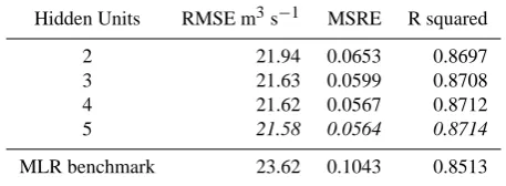
Calibration and validation performance for the four candi-date NNRFs, driven by upstream inputs, are presented in Ta-bles 5 and 6. The metric scores for Scenario B provide lim-ited evidence by which to discern the relative validity of the candidate models, with all candidates again returning simi-lar metric statistics. However, in contrast to Scenario A, one candidate model consistently achieved the best result. The 5-hidden-unit NNRF produced the best metric scores for two of the three calibration metrics, and for all validation met-rics. On this basis, its preferential selection could be argued, and this selection would be in line with previously published data-driven modelling studies in which candidate model pref-erence has been determined on the basis of consistent, best fit metric scores that represent relatively small overall per-formance gains (Kisi and Cigizoglu, 2007). It should also be

Table 6. Validation performance of candidate models for Scenario B. Best performing ANN models for each metric are in italic.

Hidden Units RMSE m3s−1 MSRE R squared

2 21.94 0.0653 0.8697

3 21.63 0.0599 0.8708

4 21.62 0.0567 0.8712

5 21.58 0.0564 0.8714

MLR benchmark 23.62 0.1043 0.8513

noted that, in this scenario, the performance of all NNRF can-didates exceed that of the MLR benchmark; highlighting the importance of non-linearity associated with river forecasting based on upstream inputs.

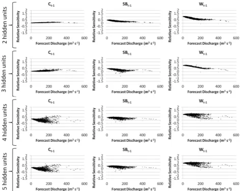
5.2 Candidate model mechanisms

Global–local relative sensitivity plots for the calibration and validation partitions of each upstream input used in each can-didate model are presented in Figs. 12 and 13. Once again, the resultant similarity of relative sensitivity patterns in the calibration and validation data subsets is to be expected given the large data record being modelled and the similarity of each subset’s hydrological characteristics as demonstrated in Fig. 7. Wt−1is the strongest driver of St, particularly at low forecast ranges, with moderate sensitivity to SBt−1also being evident. A clear mechanistic distinction between the 2- and 3-hidden-unit candidates and their 4- and 5-hidden-unit counterparts can be observed based on the coherency of their mechanisms. The 4- and 5-hidden-unit candidates dis-play low coherency, particularly at moderate to high forecast ranges, and this is particularly evident for inputs Ct−1 and Wt−1. This suggests that modelling mechanisms in the more complex candidates may be overfitting the upper-range data; a tendency that is well known when ANN-based hydrological models are used to fit heteroscedastic data (Mount and Abra-hart, 2011b). The importance of avoiding overfitting in ANN models is well known (Guistolisi and Lauocelli, 2005), and the lack of coherency in the 4- and 5-hidden-unit candidates thus raises concerns over their mechanistic legitimacy.

Low sensitivity to variation in the discharge at Ct−1 is a particular feature of the 2- and 3-hidden-unit candidates. This pattern parallels the MLR coefficients (Eq. 5) that high-light SBt−1 as the strongest model driver in the regression model. However, it contrasts with the proportional contribu-tion that each lagged, upstream discharge makes to overall discharge at St (Fig. 9). Indeed, the significant proportional contribution made by Ct−1 is minimised by the candidates – a factor that highlights the signal-based, rather than physi-cally based nature of their modelling mechanisms. Reduction in the relative sensitivity to SBt−1and Wt−1as the forecast range increases is evident in both the 2- and 3-hidden-unit candidates, and highlights the presence of non-linearity in

[image:11.595.55.280.94.179.2]

(12)

Figure 12. Global-local relative sensitivity plots for all candidate models in Scenario B:

44

local relative sensitivity plots for all candidate models in Scenario B: calibration data.

local relative sensitivity plots for all candidate models in Scenario B: Fig. 12. Global–local relative sensitivity plots for all candidate mod-els in Scenario B: calibration data.

the modelling mechanism. The high degree of stability in these plots is indicative of relatively low-complexity in the non-linearity mechanism.

In differentiating the mechanistic legitimacy of these two candidates, however, the relative sensitivity plots for Ct−1 and SBt−1are of particular interest. The increase from 2- to 3-hidden-units is accompanied by a moderate reduction in the coherency of the relative sensitivity to SBt−1at medium forecast ranges, and the existence of some negative values. To some extent, these negative sensitivity values are counter-acted by slightly higher positive sensitivity to Ct−1 at sim-ilar forecast ranges. Nonetheless, in the context of an up-stream river forecasting model, it is difficult to justify a mod-elling mechanism that acts to reduce downstream discharge forecasts as discharge increases upstream. Consequently, the legitimacy of the 3-hidden-unit candidate is difficult to ar-gue. Indeed, the 2-hidden-unit candidate appears to have the greatest mechanistic legitimacy of the candidates, combin-ing high coherency and appropriate stability in its relative sensitivity to inputs, albeit with the predictive power of Ct−1 minimised to near-zero.

5.3 Model selection

Scenario B represents a situation in which the fit metrics as-sociated with different candidate models provide only lim-ited evidence to inform model selection. On the basis of fit metrics alone, the 5-hidden-unit model appears to offer the best modelling solution as it consistently has the best scores. However, the actual performance gains are small, question-ing whether a simpler model with only marginally lower per-formance might actually be preferable. Indeed, examination of the 5-hidden-unit candidate’s internal mechanism reveals low coherency that is very difficult to legitimise over its more

Figure 13. Global-local relative sensitivity plots for all candidate models in Scenario B:

45

local relative sensitivity plots for all candidate models in Scenario B: cross-validation data.

local relative sensitivity plots for all candidate models in Scenario B: Fig. 13. Global–local relative sensitivity plots for all candidate mod-els in Scenario B: cross-validation data.

coherent and less complex NNRF counterparts. Taking into account both fit metric scores and the legitimacy of inter-nal mechanisms, the 2-hidden-unit candidate offers the best overall modelling solution. It combines high coherency and an appropriate degree of stability in its modelling mecha-nisms, with fit metric scores that are only fractionally lower than the best performing 5-hidden-unit candidate.

6 Summary

The example analysis presented in this paper demonstrates that fit metric scores alone are an insufficient basis by which to assess and discriminate between different NNRFs. The high degree of equifinality in metric scores for our candi-date models masks important differences in their complexity, mechanistic behaviour and legitimacy, which is only exposed when internal modelling mechanisms are explored. The im-portance of a mechanistic evaluation is particularly evident for Scenario B, where small improvements in metrics are as-sociated with a substantial reduction in mechanistic legiti-macy. Thus, the study responds to the issue of whether the end point of a model (i.e. its fit) is a sufficient basis by which to justify its means (i.e. the numerical basis by which the fit is achieved).

[image:12.595.49.285.62.250.2] [image:12.595.309.547.63.252.2]

(13)

[image:13.595.56.538.81.324.2]

Table 7. Example approaches to exploring and justifying ANN-based hydrological models.

ANN Component

Scope of Exploration

Example Approaches

Purpose

Inputs Structural

and Partial

Input sensitivity/saliency analysis (e.g. Maier et al., 1998; Abrahart et al., 2001; Sudheer, 2005); Partial mutual information (e.g. May et al., 2008); Leave-one-out analysis (e.g. Marti et al., 2011); Gamma function analysis (Ahmadi et al., 2009).

Optimises the input selection to ensure that only strong combinations of drivers are used.

Weights and Nodes

Structural and Partial

Exploration and regularisation of weights (e.g. Olden and Jackson, 2002; Anctil et al., 2004; Kingston et al., 2003, 2005, 2006);

Weight optimisation and reduction (e.g. Abrahart et al., 1999; Kingston et al., 2008).

Optimises network structure and may provide a basis for its physical interpretation. Inputs may sometimes be used as a control on the weights.

Node Partitions

Behavioural and Partial

Behavioural interpretation of hidden nodes (Wilby et al., 2003; Jain et al., 2004; Sudheer and Jain, 2004; See et al., 2008; Ferando and Shamseldin, 2009; Jain and Kumar, 2009).

Partitions the of the input–output relationships ac-cording to the manner in which they are processed by the different nodes present in the model struc-ture. Can support useful physical interpretation.

Network Response Function

Behavioural and Holistic

Partial derivative sensitivity analysis (Hashem, 1992*; Yeung, 2010*; Nourani and Fard, 2012).

Elucidates the mechanistic behaviours of the model. Enables legitimacy of the response func-tion to be determined and, potentially supports physical legitimisation.

Note: * Citations that are not hydrologic examples.

value as a transferrable agent that can support new hydrolog-ical insights as well as a numerhydrolog-ical tool for gaining enhanced prediction.

The current situation in data-driven modelling contrasts with the advances made by physical and conceptual mod-ellers, which centre on the development of new model eval-uation methods and incorporate mechanistic insights into model behaviour and uncertainty (e.g. Beven and Binley, 1992). As a result, data-driven modelling in general, and ANN modelling in particular, has often been viewed as a niche area of hydrological research that has had only limited success in convincing the wider hydrological research com-munity of its potential value beyond optimised curve fitting tasks. The DDMMF we have developed provides method-ological direction that has been absent from many data-driven modelling studies in hydrology. The inclusion of a re-quirement for the elucidation and assessment of modelling mechanisms within the model development process ensures that the validation of any data-driven model makes explicit both its performance, and the legitimacy of the means by which it is achieved. This aligns it more closely with the de-velopment and evaluation processes used by conceptual and physically based modellers and opens up the possibility of developing data-driven models that are dual agents of pre-diction and knowledge creation (c.f. Caswell, 1976).

Our work builds upon more than two decades of ANN-based hydrological modelling in which significant efforts have been directed towards the goal of developing more ac-ceptable and justifiable solutions (Table 7). Published explo-rations have focussed on individual structural components

of a model (i.e. the inputs, weights and units) and substan-tial progress has been made in better understanding the logic and physical plausibility of different ANN structures. How-ever, rather than having the objective of exploring the overall mechanistic behaviour of each ANN, the objective has of-ten been to optimise its structure. Only very limited research effort has been directed towards developing methods for the legitimisation of a model’s internal behaviour. This is despite recognition that the lack of availability of such methods has been a fundamental constraint to progress in the field over the last 20 yr (Abrahart el al., 2012a). By adapting a par-tial derivative sensitivity analysis method as the means by which this is achieved, we here parallel existing approaches for mechanistic model exploration that are long standing and well established within wider hydrology (c.f. McCuen, 1973). In so doing we increase the alignment between ANN model development methodologies and those applied during the development of their conceptual and physical counter-parts: an outcome that should lead to their wider acceptance. The input scenarios that we have used to exemplify the DDMMF in this paper are more simplistic than those used in many NNRFs that include an additional array of hydro-meteorological inputs with varying degrees of temporal de-pendence (c.f. Zealand et al., 1999; Dibike and Soloma-tine, 2001). Similarly, the application of a standard, back-propagation algorithm is not fully representative of the wide range of ANN variants that have been explored in NNRF studies (c.f. Hu et al., 2001; Shamseldin and O’Connor, 2001). Consequently, the relative ease with which we have been able to quantify and interpret input relative sensitivity in

(14)

this study may not be mirrored in more complex studies that use an increased number and diversity of inputs, ANN vari-ants or other forms of DDMs. Thus, developing techniques that can deliver clear mechanistic interpretation of input rel-ative sensitivity patterns in more challenging modelling sce-narios represents an important consideration for future re-search efforts. Nonetheless, the results we present serve as a clear demonstration of the dangers associated with evalu-ating ANN models on the basis of performance validation approaches alone. Indeed, in our examples we are able to show that, in order to achieve moderate performance gains, the mechanistic legitimacy of the candidate NNRFs may be substantially reduced. This finding is particularly clear in Scenario B. It also has important implications for previous river forecasting studies that have concluded that NNRFs of-fer benefits over other established techniques based on lim-ited performance gains. Indeed, an argument could be made for revisiting previous NNRF studies, and ANN-based hy-drological models more generally, to determine the extent to which their enhanced levels of performance validation are matched by their levels of mechanistic legitimacy.

7 Conclusions

This paper has argued that gaining an understanding of the internal mechanisms by which a hydrological model gener-ates its forecasts is an important element of the model devel-opment process. It has also argued that the develdevel-opment of methods for delivering mechanistic insights into data-driven hydrological models have not been afforded sufficient atten-tion by researchers. As a result, “black-box” criticisms as-sociated with DDMs persist and their potential to deliver heuristic knowledge to the hydrological community is not being fully realised. This limitation is one of several prob-lems that must be overcome if wider acceptance of DDMs by hydrologists is to be achieved (for a discussion see Tsai et al., 2013).

This study represents an important step in addressing these limitations by shifting the focus of DDMs from their ex-ternal performance to their inex-ternal mechanisms. We have presented a generalised framework that explicitly includes a mechanistic evaluation of DDMs as a fundamental part of the model evaluation process. The framework comprises a set of high-level model development and evaluation proce-dures into which different modelling algorithms can be posi-tioned. Through the development and application of a brute-force, global–local relative sensitivity analysis, we have over-come difficulties associated with quantifying relative sensi-tivity across a model’s full forecast range, when the model inputs are temporally dependent. Our adaptation of partial derivative input sensitivity analyses as a means of examining the mechanistic behaviour of an example DDM, is reflective of long-established uses of sensitivity analyses for the mech-anistic examination of hydrological models during their

de-velopment (e.g. McCuen, 1973). To an extent, this contrasts with current advances in hydrological modelling that use sen-sitivity analyses as a means of examining the causes and im-pacts of uncertainty in the outputs of existing models (e.g. Pappenberger et al., 2008). Nonetheless, it serves as a use-ful reminder of its importance as an established means for legitimising a hydrological model.

Acknowledgements. We are grateful to two reviewers and the Editor for their helpful and insightful comments which have been valuable in improving our original manuscript.

Edited by: D. Solomatine

References

Abrahart, R. J. and See, L. M.: Neural network modelling of non-linear hydrological relationships, Hydrol. Earth Syst. Sci., 11, 1563–1579, doi:10.5194/hess-11-1563-2007, 2007.

Abrahart, R. J., See, L. M., and Kneale, P. E.: Using pruning algo-rithms and genetic algoalgo-rithms to optimise neural network archi-tectures and forecasting inputs in a neural network rainfall-runoff model, J. Hydroinform., 1, 103–114, 1999.

Abrahart, R. J., See, L. M., and Kneale, P. E.: Investigating the role of saliency analysis with a neural network rainfall-runoff model, Comput. Geosci., 27, 921–928, 2001.

Abrahart, R. J., Ab Ghani, N., and Swan, J.: Discussion of “An explicit neural network formulation for evapotranspiration”, Hy-drolog. Sci. J., 54, 382–388, 2009.

Abrahart, R. J., Mount, N. J., Ab Ghani, N., Clifford, N. J., and Dawson, C. W.: DAMP: a protocol for contextualising goodness-of-fit statistics in sediment-discharge data-driven modelling, J. Hydrol., 409, 596–611, 2011.

Abrahart, R. J., Anctil, F., Coulibaly, P., Dawson, C. W., Mount, N. J., See, L. M., Shamseldin, A. Y., Solomatine, D. P., Toth, E., and Wilby, R. L.: Two decades of anarchy? Emerging themes and outstanding challenges for neural network river forecasting, Prog. Phys. Geog., 36, 480–513, 2012a.

Abrahart, R. J., Dawson, C. W., and Mount, N. J.: Partial derivative sensitivity analysis applied to autoregressive neural network river forecasting, in: Proceedings of the 10th International Conference on Hydroinformatics, Hamburg, Germany, 14–18 July 2012, p. 8, 2012b.

Ahmadi, A., Han, D., Karamouz, M., and Remesan, R: Input data selection for solar radiation estimation, Hydrol. Process., 23, 2754–2764, 2009.

American Institute of Aeronautics and Astronautics: Guide for the Verification and Validation of Computational Fluid Dynamics Simulations, AIAA-G-077-1998, Reston, Virigina, USA, 1998. Anctil, F., Michel, C., Perrin, C., and Andreassian, V.: A soil

mois-ture index as an auxiliary ANN input for stream flow forecasting, J. Hydrol., 286, 155–167, 2004.

Aytek, A., Guven, A., Yuce, M. I., and Aksoy, H.: An explicit neu-ral network formulation for evapotranspiration, Hydrolog. Sci. J., 53, 893–904, 2008.

(15)

Balci, O.: Verification, validation and testing, in: Handbook of Sim-ulation, John Wiley and Sons, Chichester, UK, 335–396, 1998. Baxter, C. W., Stanley, S. J., Zhang, Q., and Smith, D. W.:

Develop-ing artificial neural network process models: A guide for drink-ing water utilities, in: Proceeddrink-ings of the 6th Environmental En-gineering Society Specialty Conference of the CSCE, 376–383, 2000.

Beven, K. J.: Towards a coherent philosophy for modelling the en-vironment, P. R. Soc. London A, 458, 2465–2484, 2002. Beven, K. J. and Binley, A.: The future of distributed models: model

calibration and uncertainty prediction, Hydrol. Process., 6, 279– 298, 1992.

Carson, J. S.: Convincing users of a model’s validity is a challenging aspect of a modeler’s job, Ind. Eng., 18, 74–85, 1986.

Caswell, H.: The validation problem, in: Systems Analysis and Sim-ulation in Ecology, Vol. IV., Academic Press, New York, 313– 325, 1976.

Coulibaly, P., Anctil, F., and Bobe, B.: Daily reservoir inflow fore-casting using artificial neural networks with stopped training ap-proach, J. Hydrol., 230, 244–257, 2000.

Curry, G. L., Deuermeyer, B. L., and Feldman, R. M.: Siscrete Sim-ulation, Holden-Day, Oakland, California, 297 pp., 1989. Davis, P. K.: Generalizing concepts of verification, validation and

accreditation for military simulation, R-4249-ACQ, October 1992, RAND, Santa Monica, CA, 1992.

Dawson, C. W., Abrahart, R. J., Shamseldin, A. Y., and Wilby, R. L.: Flood estimation at ungauged sites using artificial neural net-works, J. Hydrol., 319, 391–409, 2006.

Dawson, C. W., Abrahart, R. J., and See, L. M.: HydroTest: a web-based toolbox of evaluation metrics for the standardised as-sessment of hydrological forecasts, Environ. Modell. Softw., 22, 1034–1052, 2007.

Dawson, C. W., Abrahart, R. J., and See, L. M.: HydroTest: further development of a web resource for the standardised assessment of hydrological models, Environ. Modell. Softw., 25, 1481–1482, 2010.

Dawson, C. W., Mount, N. J., Abrahart, R. J., and Shamseldin, A. Y.: Ideal point error for model assessment in data-driven river flow forecasting, Hydrol. Earth Syst. Sci., 16, 3049–3060, doi:10.5194/hess-16-3049-2012, 2012.

de Vos, N. J.: Echo state networks as an alternative to traditional artificial neural networks in rainfall-runoff modelling, Hydrol. Earth Syst. Sci., 17, 253–267, doi:10.5194/hess-17-253-2013, 2013.

Dibike, B. Y. and Solomatine, D. P.: River flow forecasting using artificial neural networks, Phys. Chem. Earth, 26, 1–7, 2001. Fernando, D. A. K. and Shamseldin, A. Y.: Investigation of internal

functioning of the radial-basis-function neural network river flow forecasting models, J. Hydrol. Eng., 14, 286–292, 2009. Firat, M.: Comparison of Artificial Intelligence Techniques for

river flow forecasting, Hydrol. Earth Syst. Sci., 12, 123–139, doi:10.5194/hess-12-123-2008, 2008.

Fraedrich, D. and Goldberg, A: A Methodological framework for the validation of predictive simulations, Eur. J. Oper. Res., 124, 55–62, 2000.

Giustolisi, O. and Laucelli, D.: Improving generalization of artifi-cial neural networks in rainfall–runoff modelling, Hydrolog. Sci. J., 50, 439–457, 2005.

Hamby, D. M.: A review of techniques for parameter sensitivity analysis of environmental models, Environ. Monit. Assess., 32, 135–154, 1994.

Hashem, S.: Sensitivity analysis for feedforward artificial networks with differentiable activation functions, in: Proceedings of the International Joint Conference on Neural Networks, Baltimore, USA, 7–11 June, 1, 419–424, 1992.

Helton, J. C.: Uncertainty and sensitivity analysis techniques for use in performance assessment for radioactive waste disposal, Reliab. Eng. Syst. Safe., 42, 327–367, 1993.

Hill, M. C. and Tiedeman, C. R.: Effective Groundwater Model Cal-ibration with Analysis of Sensitivities, Predictions, and Uncer-tainty, Wiley, New York, 2007.

Hipel, K. W., McLeod, A. I., and Lennox, W. C.: Advances in Box-Jenkins modeling 1. model construction, Water Resour. Res., 13, 567–575, 1977.

Holvoet, K., van Griensven, A., Seuntjens, P., and Vanrolleghem, P. A.: Sensitivity analysis for hydrology and pesticide supply to-wards the river in SWAT, Phys. Chem. Earth, 30, 518–526, 2005. Howes, S. and Anderson, M. G.: Computer simulation in geomor-phology, in: Modeling Geomorphological Systems, John Wiley and Sons Ltd, Chichester, 1988.

Hu, T. S., Lam, K. C., and Ng, S. T.: River flow time series predic-tion with a range-dependent neural network, Hydrolog. Sci. J., 46, 729–745, 2001.

Huang, W., Xu, B., and Chan-Hilton, A.: Forecasting flows in Apalachicola River using neural networks, Hydrol. Process., 18, 2545–2564, 2004.

Imrie, C. E., Durucan, S., and Korre, A.: River flow prediction using artificial neural networks: generalisation beyond the calibration range, J. Hydrol., 233, 138–153, 2000.

Jain, A. and Kumar, S.: Dissection of trained neural network hydro-logic models for knowledge extraction, Water Resour. Res., 45, W07420, doi:10.1029/2008WR007194, 2009.

Jain, A., Sudheer, K. P., and Srinivasulu, S.: Identification of phys-ical processes inherent in artificial neural network rainfall runoff models, Hydrol. Process., 18, 571–581, 2004.

Jakeman, A. J., Letcher, R. A., and Norton, J. P.: Ten iterative steps in development and evaluation of environmental models, Envi-ron. Modell. Softw., 21, 602–614, 2006.

Kingston, G. B., Maier, H. R., and Lambert, M. F.: Understanding the mechanisms modelled by artificial neural networks for hy-drological prediction, in: Modsim 2003 – International Congress on Modelling and Simulation, Modelling and Simulation Society of Australia and New Zealand Inc, Townsville, Australia, 14– 17 July, 2, 825–830, 2003.

Kingston, G. B., Maier, H. R., and Lambert, M. F.: Calibration and validation of neural networks to ensure physically plausible hy-drological modelling, J. Hydrol., 314, 158–176, 2005.

Kingston, G. B., Maier, H. R., and Lambert, M. F.: A probabilistic method to assist knowledge extraction from artificial neural net-works used for hydrological prediction, Math. Comput. Model., 44, 499–512, 2006.

Kingston, G. B., Maier, H. R., and Lambert, M. F.: Bayesian model selection applied to artificial neural networks used for water resources modelling, Water Resour. Res., 44, W04419, doi:10.1029/2007WR006155, 2008.

Kis¸i, ¨O.: River flow forecasting and estimation using different arti-ficial neural network techniques, Hydrol. Res., 39, 27–40, 2008.