XXXXX XXXX
Distance sampling detection functions: 2D or not 2D?
D.L. Borchers ∗
Centre for Research into Ecological and Environmental Modelling, The Observatory
Buchanan Gardens, University of St Andrews, Fife, KY16 9LZ, Scotland
*email:[email protected]
and
M.J. Cox
Australian Antarctic Division, Channel Highway Kingston TAS 7050, Australia
Summary: Conventionaldistancesampling(CDS)methodsassume thatanimalsare uniformly distributedinthe vicinityoflinesorpoints.Butwhenanimalsmoveinresponsetoobserversbeforedetection,orwhenlinesorpoints arenotlocatedrandomly,thisassumptionmayfail.Byformulatingdistancesamplingmodelsassurvivalmodels,we showthatusingtimetofirstdetectioninadditiontoperpendiculardistance(linetransectsurveys)orradialdistance (pointtransectsurveys)allowsestimationofdetectionprobability,andhencedensity,whenanimaldistributioninthe vicinityoflinesorpointsisnotuniformandisunknown.Wealsoshowthattimestodetectioncanprovideinformation aboutfailureoftheCDSassumptionthatdetectionprobabilityis1atdistancezero.Weobtainamaximumlikelihood estimatoroflinetransectsurveydetectionprobabilityandeffectivestriphalf-widthusingtimestodetection,andwe investigateitspropertiesbysimulationinsituationswhereanimalsarenonuniformlydistributedandtheirdistribution isunknown.Theestimatorisfoundtoperformwellwhendetectionprobabilityatdistancezerois1.Itallowsunbiased estimatesofdensitytobeobtainedinthiscasefromsurveysin whichtherehasbeenresponsivemovementpriorto animals coming within detectable range.When responsivemovement continues within detectable range,estimates may be biasedbutarelikelyless biasedthanestimates frommethods thatassuming noresponsivemovement.We illustratebyestimatingprimatedensityfromalinetransectsurveyinwhichanimalsareknowntoavoidthetransect line,andashipboardsurveyofdolphinsthatareattractedtoit.
1. Introduction
There are two main distance sampling methods: line transects and point transects. On line
transect surveys observers traverse lines and record the perpendicular distances from the line
to detected individuals, while on point transect surveys observers survey from points and
record the radial distances to detected individuals. Observers may also record the locations
in the plane of detected individuals, and other covariates. See Marques et al. (2010) and
Buckland et al. (2001) for an overview of distance sampling methods.
Two key assumptions of distance sampling are (i) that the distribution of distances from
samplers (lines or points) to individuals in the vicinity of the samplers is known (usually
assumed uniform for line transects and triangular for point transects) and (ii) that detection
of individuals at distance zero is certain (Buckland et al., 2001). Assumption (ii) is referred
to as the “g(0) = 1” assumption in distance sampling literature, whereg(x) is the probability
of detecting an individual that is at perpendicular distance x in the case of line transects,
and radial distance x in the case of point transects. In this paper we use p(x) rather than
g(x) for the detection probability function.
We are interested in developing methods that do not require assumption (i) in particular,
because on some surveys it may not be possible to meet this assumption. There are two main
circumstances in which this is the case. The first is when samplers (lines or points) cannot
be placed randomly, as may be the case in a jungle where observers are restricted to moving
along paths, and we consider a visual line transect survey of primates where this was the
case. The second is where animals move in response to an observer prior to being detected,
and we consider a shipboard dolphin survey in which this was the case.
We show below that distance sampling methods that use times to detection do not require
assumption (i) and that these methods are kinds of removal methods (see Seber, 1982;
And since removal methods require neither assumption (i) nor assumption (ii), we investigate
the extent to which use of times to detection allows assumption (ii) to be relaxed as well.
While times to detection are not used by current distance sampling methods, something
akin to them were used in some old line transect survey models and we briefly review the
reasons that their use was abandoned. But first we consider removal methods as these provide
some insights for distance sampling surveys with time to detection.
1.1 Removal models as survival models
Removal methods involve repeated sampling and removing animals from a population when
they are detected or captured. (We refer to detection, capture and removal as “detection”
henceforth.) In the simplest model, all animals are assumed to be equally detectable and
sampling effort is assumed to be the same on each occasion.
We can formulate a removal method with occasions 1, . . . , T as a discrete time survival
process with constant detection probabilitypand an unknown number of right-censored
indi-viduals. In this case the “survivor function” (the probability of not being detected by occasion
(t−1)∈ {1, . . . ,(T−1)}) isS(t−1) = (1−p)t−1 and the probability of being detected at time
(occasion) t∈ {1, . . . , T} isf(t) =S(t−1)p (i.e. t has a geometric distribution). The
likeli-hood for the abundanceN and detection probabilityp, given thatntindividuals were detected
at time t (t = 1, . . . , T) is multinomial: L(N, p) = N!
(N−n)!QT
t=1nt!
S(T)N−nQn
i=1S(ti−1)p,
where n = P
tnt and N −n is the unknown number of censored survival times. The focus
of inference is the number of censored times. Although it is not usually formulated as a
discrete survival model, the simple removal method likelihood (see Equation 5.4 on page 76
of Borchers et al., 2002, for example) is identical to the equation above.
The link between removal methods and distance sampling methods becomes apparent
when we consider the continuous-time analogue of the discrete-time removal model – which
of detection, h. In this case the survivor function at time t is S(t;h) = exp{−Rt
0 h du} =
exp{−th}and the probability density function (pdf) of thendetection times, given detection,
is f(t|t6T) =Qn
i=1
S(ti;h)h
1−S(T;h), where t 6T indicates thatt1, . . . , tn are all less than or equal
to T. Note that 1−S(T;h) is the probability of detection by time T, which we denote p.
The corresponding likelihood function for the survey is L(N, h) = B(n;N, p)Qn
i=1
S(ti)h
p ,
where B(n;N, p) is a binomial probability mass function (pmf) with index N and “success”
probability p, evaluated atn.
Suppose now that in addition to the time that an individual has been at risk of detection
(t), the detection hazard depends on a continuous individual random effect x with pdf
π(x;φ) and parameter vector φ. We assume that individuals’ xs are independent draws
from this distribution. The detection hazard is nowh(t, x;β), whereβis a vector of unknown
parameters, the survivor function is S(t, x;β), and detection probability, conditional onx is
p(x;β) = 1−S(T, x;β) = 1−exp{−RT
0 h(u, x;β)du}. The mean detection probability in
the population is p·(β,φ) = Ex[p(x;β,φ)] =
R
π(u;φ)p(u;β)du, where integration is over
the survey region. The likelihood function can now be written as
L(N,β) = B(n;N, p·(β,φ))
n
Y
i=1
π(xi|ti 6T)f(ti|xi, ti 6T)
= B(n;N, p·(β,φ))
n
Y
i=1
π(xi;φ)p(xi;β)
R
π(u;φ)p(u;β)du
S(ti, xi;β)h(ti, xi;β)
p(xi;β)
(1)
=
N n
[1−p·(β,φ)]N−n
n
Y
i=1
π(xi;φ)S(ti, xi;β)h(ti, xi;β) (2)
The term [1−p·(β,φ)]N−n is for the unknown number (N −n) of censored survival times.
1.2 Distance sampling models as survival models
Although they are traditionally treated as instantaneous surveys, distance sampling surveys
seldom really are. An individual at (perpendicular or radial) distance x is in view for some
period (of length T say), and at time 0 6 t 6 T it has some hazard h(t, x;β) of being
of recording only the locations of individuals when first detected, is used. In this case, one can
consider a distance sampling survey to be a removal survey of the sort described immediately
above, and hence also as a kind of survival model survey.
Indeed, the conventional distance sampling full likelihood is identical to Equation (1) with
the random effect x being perpendicular distance (in the case of line transects) or radial
distance (in the case of point transects), except that with distance sampling (a) the random
effect distribution π(xi;φ) is treated as known, and (b) the term with detection times
(f(ti|xi, ti 6 T) = S(ti, xi;β)h(ti, xi;β)/p(xi;β)) is omitted - see Buckland et al. (2004),
Equation (2.33) or Borchers et al. (2002), Equation (7.10). We are concerned in this paper
with situations in which it is not reasonable to treat π(xi;φ) as known, and we show below
that f(ti|xi, ti 6T) is useful for estimating it.
Omitting f(ti|xi,t 6 T) from distance sampling likelihoods reduces the data from two
dimensions (x and t) to one dimension (x) and as a result π(xi;φ) and p(xi;β) are
con-founded: without f(ti|xi,t 6 T) they appear only as a product in Equation (1). This begs
the question “Why are conventional distance sampling detection functions one dimensional?”.
In the case of line transect surveys, the answer can be found in a landmark paper by Hayes
and Buckland (1983).
They considered line transect detection function models that included forward distances.
(Using forward distance, y, is equivalent to using times to detection if observers move at
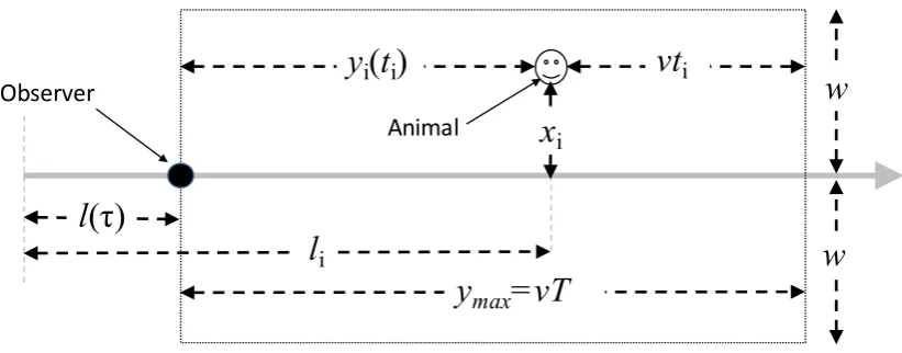
constant speed, v, since y = ymax −vt - see Figure 1.) These are two-dimensional (2D)
line transect detection function models (with forward distance y as well as perpendicular
distance, x) and the key question here is why 2D detection models were abandoned.
[Figure 1 about here.]
Hayes and Buckland (1983) considered the 2D detection models of Hayne (1949), Eberhardt
models, Hayes and Buckland (1983, p 33) conclude that “none of the models appears to
be founded upon realistic assumptions.” They went on to develop a survival model for the
detection process (although they did not call it a survival model), with a detection hazard
that depends on forward and perpendicular distance.
The key conclusion of Hayes and Buckland (1983) with regard to density estimators ( ˆD)
from 2D hazard models was (p39) “We do not believe that the estimator ˆD will be robust to
the form arbitrarily chosen for [the hazard function] when observed radial distances are used
for estimation.” (The 2D models they considered used radial and perpendicular distances,
rather than forward and perpendicular distances.) They went on to develop a new form of 1D
(perpendicular distance only) detection function (the now well-known “hazard rate” form)
based on their survival model, and showed that this form is obtained from a variety of forms
for the hazard function.
Hayes and Buckland (1983) concluded that the weakness of the 2D models they looked at
was that they were “arbitrary” and “founded on unrealistic assumptions”. But other 2D
dis-tance sampling models had been used successfully before 1983 (Schweder, 1974, for example)
and have been used successfully since. Examples include (Schweder, 1990), Schweder et al.
(1996), Schweder et al. (1997), Schweder et al. (1999), Skaug and Schweder (1999), Okamura
(2003), Skaug et al. (2004), Okamura et al. (2003), Okamura et al. (2006), Okamura et al.
(2012), Borchers et al. (2013), Langrock et al. (2013) and Borchers and Langrock (2015).
These papers used a variety of more flexible hazard function forms than the models considered
by Hayes and Buckland (1983), including models that allow p(0) <1. However, all of them
concern individuals that become available and unavailable for detection stochastically while
within detection range. In a similar vein, Solymos et al. (2013) and Amundson et al. (2014)
developed models for point transect surveys that use times to detection, for individuals that
dealing with time intervals of different lengths, or continuous time. We develop 2D distance
sampling models without stochastic individual availability here, and apply them with one of
the hazard models proposed by Hayes and Buckland (1983) and two of the hazard models
proposed by the authors listed above. The detection hazard formulation above also provides
a mechanism for extending models like those of Solymos et al. (2013) and Amundson et al.
(2014) to deal with continuous time and/or intervals of different lengths.
1.3 Detection probability at distance zero
Conventional distance sampling methods assume that p(0) = 1. One can build this into 2D
detection function models by choosing an appropriate hazard function form - as did Hayes
and Buckland (1983), for example. Or one can use a hazard function form that does not
require the p(0) = 1 assumption, as did Langrock et al. (2013), for example.
Thinking of distance sampling data as removal (or survival) data, one would expect that it
is possible to estimate abundance without assuming thatp(0) = 1 - since no such assumption
is required for estimation from removal method data. On the other hand, the simple (constant
p) removal method performs poorly unless a relatively high proportion of the population is
detected (see Seber, 1982, Table 7.3, for example), i.e., unless S(T) is close to 1. So one
might also expect poor performance from 2D distance sampling estimators unless p(0) =
p(x= 0;β) = 1−S(t, x= 0;β) is close to 1. We consider this further below.
2. Distance sampling likelihood
Distance sampling observations arise only within some maximum searched distance w of
samplers (lines or points) and conventional distance sampling estimators of density and
abundance commonly use design-based methods for drawing inferences outside of this
“cov-ered region”, while model-based methods of inference are used within the cov“cov-ered region.
are unknown, are beyond the control of the surveyor, and are estimated on the basis of a
model for the detection function (with some unknown parameters) whereas the probability of
individuals being in the covered region can be determined by design. Here we are concerned
with inference within the covered region.
On a line transect survey, the location of individual i is conveniently expressed as xi, its
distance from the line, and li, its distance along the line (see Figure 1). An observer moves
along the line at constant speed v, such that her location along the line at time τ is l(τ),
with a window of half-width w and lengthymax =vT moving with her. Each individual has
its own time coordinate (Ti for individuali) which is set to 0 when the observer is a distance
ymax short of li, and at time Ti = ti it is at forward distance yi(ti) ahead of the observer
(Figure 1). So for line transects, the observer-centric coordinates are (xi, yi(ti)).
As with conventional line transect models, we assume that the probability of detecting
individual i at perpendicular distance xi from the line does not depend on its distance li
along the line. (One can add covariates to the detection hazard to allow it to vary with
distance along line.) This implies that the detection hazard function depends on xi and time
in view (ti), but not on li, so that it can be written as h(xi, yi(ti)) and the survivor function
can be written as S(ti, xi). (The time that individuals at the start of the line withli < ymax
are in view is less than T and this should strictly be taken account of in the likelihood. This
“end effect” is usually negligible.) In the case of point transects, both the observer and the
animals are assumed to be stationary until detection, so that unless the detection hazard
varies with time, it can be written simply ash(xi), where in this casexi is the radial distance
of animal i from the observer.
2.1 Conditional likelihood
Inference within the covered region is conventionally based on the conditional likelihood,
above (which includes a binomial probability model for n). This is to avoid having to model
the distribution outside of searched strips or circles (Borchers and Burnham, 2004). The
conditional likelihood is Equation (1) without the leading binomial pdf term:
L(β|n) = fx|n(x|n)ft|x(t|x,t6T)
=
( n
Y
i=1
π(xi;φ)p(xi;β)
R
π(u;φ)p(u;β)du
) ( n
Y
i=1
S(ti, xi;β)h(ti, xi;β)
p(xi;β)
)
(3)
wherex= (x1, . . . , xn),t= (t1, . . . , tn) andt 6T indicates that all oft1, . . . , tn are less than
or equal to T. Here fx|n(x|n) is the conditional likelihood, but allowing a more general form
for π(xi;φ) than is conventionally used. With CDS, uniform object density within w of the
observer is usually assumed, so that for line transects π(xi;φ) =C for some constantC, and
C cancels in fx|n(x|n), leaving Qip(xi)/
R
p(x)dx, which is the CDS conditional likelihood
for line transects (see Buckland et al., 2001). Similarly, with uniform object density for point
transects π(xi;φ)∝xi (see Buckland et al., 2001) giving the CDS point transect conditional
likelihood Q
i
xip(xi)/
R
xp(x)dx . It is standard practice with distance sampling inference
not to use times to detection and so CDS likelihoods do not involve the component ft|x(t|x).
We do include times to detection and ft|x(t|x), and it is this that enables us to deal with
unknown π(xi;φ), responsive movement prior to detection, and to some extent uncertain
detection at distance zero.
2.2 CDF and PDF of detection times
The shape of the pdf of detection time t at distance zero, given t6T, i.e.ft|x(t|x, t6T) =
S(ti,xi)h(ti,xi)
p(xi (omitting β for brevity), turns out to be somewhat informative about p(0). If
p(0) = 1 then ft|x(t|0, t 6 T) must approach zero as t → T, as in this case no animals
at distance x = 0 survive detection beyond T (forward distances y < 0 in the case of line
(x= 0, y = 0) for line transects). This in turn means that ft|x(t|0, t 6T) must have a mode
at t6T (y >0). Conversely, if it does not then this implies that p(0) is less than 1.
The cumulative distribution function (CDF) of t is the scaled probability that an object
at x survives detection up to time t: Ft|x(t|x) = S(t, x)/
RT
0 S(t, x)dt. This is analogous to
the removal method CDF and as with removal methods, when Ft|x(t = T|x) is not close
to 1 (i.e. when, by the end of the period in which animals are at risk of removal/detection,
not a large fraction of the available population has been removed/detected), estimation of
the proportion of the available population that has been removed/detected (and specifically
p(0) =Ft|s(t =T|0) in the present context), can not be done reliably.
The mean pdf of t, given detection, is useful for visually assessing goodness of fit in the
t dimension. For line transects this is Ex[ft|x(t|x)] =
Rw
x ft|x(t|x, t 6 T))π(x;φ)dx where
ft|x(t|x, t6T) is the pdf of t given distance x and detection.
3. Detection hazards and perpendicular distance distributions
We now focus on line transect surveys. Although our models are formulated above in terms
of detection times, when observers move at constant speed it is convenient to work in terms
of forward detection distances (y) rather than times, which we do henceforth. We use one
of the hazard forms (model hHB below) proposed by Hayes and Buckland (1983) as well as
the exponential power and inverse power hazard models that were used by Langrock et al.
(2013) (hEP andhIP). We also generalisehHB to allowp(0) <1 (hazardhHB2) and the latter
as follows (βj >0 for all j):
hHB(x;β) = β1(x2+y2)−(β2+2)/2 hHB2(x;β) =β1(x2+ (y+β3)2)−(β2+2)/2
hIP(x;β) =β1
( 1 + x β2 2 + y β2
2)−(β3+1)/2
hEP(x;β) =β1exp
( x β2 β3 + y β2
β3)
hIP2(x;β) =β1
( 1 + x β2 2 + y β4
2)−(β3+1)/2
hEP2(x;β) = β1exp
( x β2 β3 + y β4
β3)
The hazard hHB has p(0) = 1, whereas the other hazards allow p(0) < 1. We use slightly
different forms for hEP and hIP than do Langrock et al. (2013), in that we allow β1 to be
greater than 1 (because our hazard functions are rates, not probabilities).
As is done with CDS methods, we use the absolute value of perpendicular distance so that
x > 0, and we right-truncate x at a distance w from the transect line. We consider these
forms for π(x;φ) (φ1 >0;−∞6φ2 6∞):
πU(x;φ) =
1
w πHN(x;φ) = e
−x2 2φ2
1
Z w
0 e−
x2
2φ2 1dx
−1
πN(x;φ) =e
−(x−φ2)2 2φ21
(
Z w
0 e−
(x−φ2)2 2φ21 dx
)−1
πCN(x;φ) =
1−e−
x2
2φ21 w−
Z w
0 e−
x2
2φ21dx
−1
Model πU corresponds to no responsive movement, πHN allows for attraction to the transect
line, πCN for avoidance and πN for attraction or avoidance.
4. Model selection, diagnostics and interval estimation
The focus of inference is the inclusion probability in the covered region and the key
quan-tity for this in the case of line transects is the effective strip half-width, defined as ˜w =
wRw
0 p(x)π(x)dx
, wherep(x) = 1−S(T, x) andT is the maximum time animals are within
detectable range. (The inclusion probability is RL
0 2 ˜wdl/(2wL) = ˜w/w, where integration is
along the transect and L is the total transect length.) The variance-covariance matrix of
model parameters is estimated using the inverse Hessian matrix obtained by maximising
the Delta Method (see Oehlert, 1992, for example). Confidence intervals for ˜w are obtained
assuming log-normality of the estimator.
Models can be selected on the basis of their AIC values, and goodness of fit in the
perpendicular distance and forward distance dimensions assessed by visual inspection of
model fits in each dimension and Q-Q plots together with Kolmogarov-Smirnov (KS) and
Cramer-von Mises (CvM) goodness of fit test statistics.
5. Applications
We estimate ˜wfor two surveys, both of which are believed to involve be substantial responsive
movement by animals prior to detection. The data are shown in Figure 2.
[Figure 2 about here.]
The first dataset has 127 detections of primates from a visual survey conducted by three
sets of trained observers walking previously cut line transects in primary tropical rainforest at
an elevation of 200-600m above sea level. The primates are believed to avoid the surveyors by
moving some distance away from the paths, and the distribution of perpendicular distances
of detected animals displays a mode at around 15m from the transect line (Figure 3).
[Figure 3 about here.]
The second dataset has 76 detections of dolphin groups by one set of observers (the “primary
platform”) on a shipboard visual survey. This survey used two independent observers and
data from both observers were analysed using mark-recapture distance sampling (MRDS)
methods (see Burt et al., 2015, for an overview of these methods) by Ca˜nadas et al. (2004).
They concluded that there was substantial attraction of schools towards the transect line.
The perpendicular distance data have a mode at, or very close to distance zero (Figure 4).
For each of these surveys, we estimate ˜w by maximising Equation (3) and also by
max-imising the CDS likelihood, obtained by dropping ft|s(t|s) from Equation (3) and setting
π(x;φ) = C to reflect the CDS assumption that objects are distributed uniformly forx6w.
CDS estimates were obtained using the R package Distance (Miller, 2015).
5.1 Primate survey results
The primate data were truncated at perpendicular distance w = 0.03 km, resulting in 4
detections being discarded. All models with πU had significantly bad fit in the x dimension.
Among models with non-significant goodness of fit statistics at the 5% level, model pair
(hIP, πN) was selected on the basis of AIC, with the next best model (hEP, πN) having an
AIC larger by 8.6. However, parametersβ2 andβ3of model (hIP, πN) were found to be highly
correlated (estimated correlation >0.999) and estimates from simulations using this model
did not converge properly in 40% of cases. We therefore fitted a reduced version of (hIP, πN),
which we call (hIP0, πN), in which the scale parameter β2 is fixed at 1. This resulted in a
model with lower AIC than (hIP, πN) and so we base inference on model (hIP0, πN). (The
point estimates of ˜w of these two models differ by less than 0.1%) Goodness of fit tests
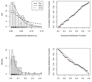
give p-values of 0.72 (CvM) and 0.63 (KS) in the x dimension and 0.75 (CvM) and 0.76
(KS) in the ydimension. The fits of the chosen model in perpendicular and forward distance
dimensions are shown in Figure 3. The chosen model has p(0) = 1.
A common, if ad-hoc way of dealing with data demonstrating avoidance of the transect
lines, is to fit the hazard rate model of Hayes and Buckland (1983) (which is equivalent to the
2D modelhHB in the perpendicular distance dimension). This model has a flat shoulder and
although it fits poorly to these data, the rationale for using it in the presence of avoidance
is that it ‘undoes’ the avoidance to some extent by averaging through the region from which
animals have fled close to the line and to which they have fled farther from the line. This
data (which CDS models do not use) in addition to perpendicular distance data, with πU
(which is consistent with the CDS assumption of uniform animal density). This fitted model
has an AIC that is larger by 54.9 than the preferred model (hIP, πN).
[Figure 5 about here.]
The selected model (hIP0, πN) has an estimated ˜w of 0.018 with a coefficient of variation
(CV) of 12.5% and 95% confidence interval (CI) of (0.014, 0.023). The CDS model has an
estimated ˜w 28% larger at 0.023, with a CV of 5.8%. Since estimated density is inversely
proportional to ˜w (density is estimated as ˆD = n/(2wL)), the CDS model gives a densityb˜
estimate that is some 22% smaller than that from the selected 2D model.
The differences between the CDS estimate, which uses only perpendicular distance data and
the estimates from our method, which uses 2D data (perpendicular and forward distances),
are consistent with the CDS estimator not accounting adequately for the apparent avoidance
of transect line by primates, and the 2D method accounting for the avoidance, albeit at the
cost of additional variance due to estimating 2D hazard parameters and φ.
5.2 Dolphin survey results
The dolphin data were truncated at perpendicular distance w = 0.15 km, resulting in two
detections being discarded. Models were fitted to these data with distance distribution models
πU and πHN. All the models with πU had significantly bad fit. Among the models that did
not have significantly bad fit, model (hHB, πHN) was selected on the basis of AIC. All models
that allow p(0) < 1 had substantially worse AICs than model (hHB, πHN). Goodness of fit
tests give p-values for the selected model of 0.79 (CvM) and 0.89 (KS) in thexdimension and
0.24 (CvM) and 0.42 (KS) in they dimension. The fits of the chosen model in perpendicular
and forward distance dimensions is shown in Figure 3.
CDS methods were used to fit half-normal and hazard rate detection function models and
Model (hHB, πN) has an estimated ˜w of 0.107 with a CV of 8.9% and 95% CI of (0.089,
0.127). The CDS model has an estimated ˜wsome 40% smaller at 0.064 with a CV of 18.8%,
generating a density estimate that is 67% larger than that from model (hHB, πN).
Ca˜nadas et al. (2004) obtained a density estimate of 0.123 schools per square nautical
mile using MRDS methods that assume no unmodelled heterogeneity (no variables affecting
detection probability of the two sets of observers that are not accounted for in the model).
This will be a negatively biased estimate of density if there is unmodelled heterogeneity (see
Burt et al., 2015, for a summary of this and related issues), and it is frequently the case that
there is unmodelled heterogeneity on MRDS surveys. While there are “point independence”
MRDS methods that relax the assumption of no unmodelled heterogeneity, these require
uniform distribution of perpendicular distances of animals from the transect line and produce
biased estimates in the presence of responsive movement (see Burt et al., 2015). Ca˜nadas
et al. (2004) also fitted a CDS model to the data and this produced an estimate of density
5.9 times larger than that from the MRDS method. The CDS estimate is positively biased
in the presence of attraction to the transect line. Believing there to be attraction to the line,
Ca˜nadas et al. (2004) chose what they believed to be the lesser of two evils and assumed no
unmodelled heterogeneity (and hence a negatively biased estimate of density if unmodelled
heterogeneity exists).
The estimated density from our method is 0.21 – almost double the MRDS estimate and
less than a third as big as the CDS estimate of Ca˜nadas et al. (2004). This is consistent with
the MRDS estimate being negatively biased (as is likely, due to unmodelled heterogeneity)
and the CDS estimate being positively biased due to responsive movement. We do not claim
that our estimator from model (hHB, πHN) is unbiased in this case, because it seems quite
likely that p(0) is less than 1 (Ca˜nadas et al., 2004, estimated it to be 0.79) due to animals
are detections very close to (x = 0, y = 0), as is evident from Figures 2 and detections
at (x = 0, y = 0) are consistent with p(0) < 1. But sample size is small and this may give
inadequate power to detectp(0) <1. In addition, the 2D method developed here assumes that
x does not change while animals are in view before they are detected, and this assumption
may be violated for these data (although it is unclear how much this would bias estimates)
Nevertheless, as with the primate data analysis, the difference between the CDS estimate
and the 2D method estimate is consistent with the 2D method being able to account for
nonuniform distribution in the perpendicular distance dimension (attraction to the transect
line in this case) and the CDS estimator not being able to do so.
We investigate by simulation below, the performance of the 2D method in the presence of
unknown non-uniform animal distribution, and compare its performance to CDS estimators.
6. Simulation study
We consider two simulation scenarios: S1 treats the 2D model fitted to the primate data
as truth, S2 treats the 2D model fitted to the dolphin data as truth with simulated data
drawn from (hIP0, πN) in S1 and (hHB, πHN) in S2. For all simulation scenarios we estimate
˜
w using our 2D method and using a CDS estimator. We measure performance in terms of
estimated ˜w relative bias and 95% CI coverage probabilities. For each scenario we simulate
1,000 surveys, with each survey having a simulated sample size equal to that of the data
sets, i.e. for simulation scenario S1 n = 127, and simulation scenario S2n = 76.
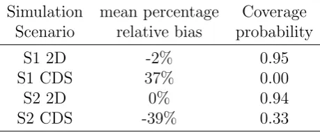
The 2D model estimator of ˜w is very nearly unbiased for S1 and unbiased for S2. In both
scenarios the 95% confidence interval estimates have coverage close to their nominal level,
while the CDS estimator has both substantial bias and very poor coverage probabilities
(Table 1).
In the case of the dolphin data, where it is likely that p(0) is less than 1, we explored the
data from our fitted model (hHB,πHN) and then shifted the origin in thetdimension forward
(i.e reduced the time individuals are in view) until p(0) was at a given value less than 1 (see
below), and then fitted model (hHB2,πHN), which allowsp(0) <1, to each of 1,000 simulated
datasets. We did this for p(0)∈ {0.9,0.8,0.7,0.6}. In all cases we foud ˆp(0) to be negatively
biased, with bias ranging from -12% to -22%. Although this is too small a simulation study
to conclude that 2D detection function models are ineffective for p(0) estimation, we would
not recommend using them for this purpose without further investigation.
[Table 1 about here.]
7. Discussion and Conclusions
We have shown that when animals are not distributed uniformly with respect to distance
from the line on line transect surveys, unbiased estimates of ˜w can be obtained from 2D
estimators that use forward distance or time to detection data as well as perpendicular
distance, and that in such cases CDS estimators may be unreliable. The 2D estimators may
be biased if there is responsive movement while within detectable range, but as the 2D model
accommodates non-uniform distribution, it is likely that 2D estimators will be less biased
than CDS estimators in this case.
We have also shown that use of forward detection distance data and 2D inference methods
provides some information on whether the key CDS assumption that p(0) = 1 has been
violated. If ft|x(t = T|x = 0; ˆβ) = 0, this indicates that no objects “survive” detection at
x = 0, i.e. that p(0) = 1. Conversely, if ft|x(t = T|x = 0; ˆβ) is greater than zero, some
animals avoid detection altogether and p(0) < 1. In principle p(0) can be estimated by
1−S(t = 0, x; ˆβ), where ˆβ is the MLE of β, but this should be done with care as small
sample size may compromise the reliability of p(0) estimation. The dolphin data are a case
the analysis of Ca˜nadas et al. (2004), that p(0) < 1, and the histogram in Figure 2 shows
detections very close to zero forward and perpendicular distance, but the best model by AIC
is one with p(0) = 1. We consider the 2D method to be reliable when p(0) is equal to, or
close to 1, but it has limited ability to deal with p(0) <1. Recalling that the 2D line transect
estimator can be seen as kind of removal method estimator, and that removal methods do
not work well unless a large fraction of the population is removed, we believe these methods
should be used with caution if p(0) may be substantially less than 1. With large enough
sample size, inspection of the distribution of forward distances may be informative in this
regard; if the distribution of forward distances of detections close to the line does not have
a mode at y >0, this would suggest thatp(0) is less than 1.
We have not addressed the issue of how representative density within strips is of density
overall when there in nonuniform animal distribution, and this is not something that can
be inferred reliably from within-strip data alone. If strips are located randomly and
nonuni-formity is a consequence of responsive animal movement that does not involve any animals
moving into or out of strips, then density within strips is representative of density outside
strips. Nonuniform density can also arise from nonrandom placement of transects, even in
the absence of responsive movement to observers. In some cases it may be reasonable to use
estimated density at the outer edge of strips as representative of density outside strips, but
in general, drawing inferences about density outside strips from estimates of density in strips
may be unreliable in the presence of nonuniform distribution within strips. Marques et al.
(2010a) discuss these issues further.
We have not investigated use of times to detection with point transects. Marques et al.
(2010a), Cox et al. (2011) and Arranz et al. (2014) showed how radial distance and angle
can be used to estimate density in the presence of nonuniform animal distribution. But if
in density, then change in detection probability and change in density with distance are
confounded even when detection angles are used. Time to detection data have the potential
to deal with this. However, the methods of this paper assume that animals are stationary
while within detectable distance and for most species, for any but very short survey times T,
this is not a reasonable assumption for point transects. And with very short survey times,
times to detection data are rather uninformative
The 2D detection function estimation method developed in this paper gives
conservation-ists, managers, and others wanting to estimate animal abundance and density from line
transect surveys a new tool for situations in which there is unknown object distribution
within searched strips or circles. While it requires time to detection or (for line transects)
forward distance at detection, these data are often quite easy to gather and we recommend
that they be gathered as a matter of course where this is possible.
Finally, we return to the question posed in the title of this paper: should distance sampling
detection function models remain 1D or move to 2D? Although time to detection data are in
principle informative aboutp(0), our limited simulations suggest that when p(0) is not close
to 1 and sample size is not large, estimation of p(0) may not be reliable, and MRDS methods
are probably preferable. An obvious extension of the methods of this paper would be the
incorporation of time to detection data in MRDS models, but that is beyond the scope of
this paper. On the other hand, we have shown the utility of 2D distance sampling data for
line transect surveys when the CDS assumption that animals are uniformly distributed in
the vicinity of observers is violated. We believe that unless the distribution of distances to
individuals is known with confidence, distance sampling detection functions should be 2D,
not 1D, as substantial bias can result from an incorrect assumption about the distribution.
Moreover 2D detection functions can be used to investigate whether the observed data is
Supplementary Materials
The R code and datasets used to do the analyses in this paper can be found on github at
https://github.com/david-borchers/LT2D .
Acknowledgements
We are grateful to Matthew Nowak from the Sumatran Orangutan Conservation Programme
(SOCP) for allowing us to use the primate survey data from the Jantho Reintroduction
Station. The initial survey was developed by Matthew Nowak and Serge Wich (Liverpool
John Moores University) and then undertaken by the SOCP with funding from Chester Zoo.
We are also grateful to the North Atlantic Marine Mammal Commission (NAMMCO) and
the Faroese Museum of Natural History for allowing us to use the dolphin survey data from
NASS95. MJC was funded by Australian Research Council grant FS110200057.
References
Amundson, C., J. Royle, and C. Handel (2014). A hierarchical model combining distance
sampling and time removal to estimate detection probability during avian point counts.
The Auk 131(4), 476–494.
Arranz, P., D. L. Borchers, N. Aguilar de Soto, M. P. Johnson, and M. J. Cox (2014, April).
A new method to study inshore whale cue distribution from land-based observations.
Marine Mammal Science 30(2), 810–818.
Borchers, D. and R. Langrock (2015). Double-observer line transect surveys with
markov-modulated poisson process models for animal availability. Biometrics DOI:
10.1111/biom.12341.
Borchers, D. L., S. T. Buckland, and W. Zucchini (2002). Estimating Animal Abundance:
Closed Populations. Springer.
S. T. Buckland, D. R. Anderson, K. P. Burnham, J. L. Laake, D. L. Borchers, and L. J.
Thomas (Eds.), Advanced Distance Sampling. Oxford University Press.
Borchers, D. L., W. Zucchini, M. P. Heide-Jorgensen, A. Canadas, and R. Langrock (2013).
Using hidden markov models to deal with availability bias on line transect surveys.
Biometrics 69, 703–713.
Buckland, S., C. Oedekoven, and D. Borchers (2015). Model-based distance sampling.
Journal of Agricultural, Biological, and Environmental Statistics, 1–18.
Buckland, S. T., D. R. Anderson, K. P. Burnham, J. L. Laake, D. L. Borchers, and L. J.
Thomas (2001). Introduction to Distance Sampling. Oxford: Oxford University Press.
Buckland, S. T., D. R. Anderson, K. P. Burnham, J. L. Laake, D. L. Borchers, and L. J.
Thomas (2004). Advanced Distance Sampling. Oxford: Oxford University Press.
Burnham, K. P. (1979). A parametric generalization of the hayne estimator for line transect
sampling. Biometrics 35, 587–595.
Burnham, K. P. and D. Anderson (1976). Mathematical models for non-parametric inference
from line transect data. Biometrics 32, 325–336.
Burt, M., D. Borchers, K. Jenkins, and T. Marques (2015). Using mark-recapture distance
sampling methods on line transect surveys. Methods in Ecology and Evolution 5, 1180–
1191.
Ca˜nadas, A., G. Desportes, and D. Borchers (2004). The estimation of the detection function
and g(0) for short-beaked common dolphins (Delphinis delphis), using double-platform
data collected during the NASS-95 Faroese survey. Journal of Cetacean Research and
Management 6, 191–198.
Cox, M. J., D. L. Borchers, D. A. Demer, G. R. Cutter, and A. S. Brierley (2011).
Estimating the density of antarctic krill (Euphausia superba) from multi-beam
Society: Series C (Applied Statistics) 60(2), 301ˆa ˘A¸S316.
Eberhardt, L. (1978). Transect methods for population studies. Journal of Wildlife
Management 42, 1–31.
Hayes, R. J. and S. T. Buckland (1983). Radial-distance models for the line-transect method.
Biometrics 39, 29–42.
Hayne, D. (1949). An examination of the strip census method for estimating animal
populations. Journal of Wildlife Management 13, 145–157.
Langrock, R., D. L. Borchers, and H. J. Skaug (2013). Markov-modulated nonhomogeneous
poisson processes for modeling detections in surveys of marine mammal abundance.
Journal of the Americal Statistical Association 108, 840–851.
Marques, T., S. Buckland, D. Borchers, E. Rexstad, and L. Thomas (2010). Distance
sampling. In M. Lovric (Ed.), Springer’s International Lexicon of Statistical Science,
pp. 398–400. Springer.
Marques, T. A., S. T. Buckland, D. L. Borchers, D. Tosh, and R. A. McDonald (2010a).
Point transect sampling along linear features. Biometrics 66, 1247–1255.
Miller, D. L. (2015). Distance: Distance Sampling Detection Function and Abundance
Estimation. R package version 0.9.4.
Oehlert, D. (1992). A note on the delta method. The American Statistician 46, 27–29.
Okamura, H. (2003). A line transect method to estimate abundance of long-diving animals.
Fisheries Science 69, 1176–1181.
Okamura, H., T. Kitakado, K. Hiramatsu, and M. Mori (2003). Abundance estimation of
diving animals by the double-platform line transect method. Biometrics 59, 512–520.
Okamura, H., S. Minamakawa, and T. Kitakado (2006). Effect of surfacing patterns on
abundance estimates of long-diving animals. Fisheries Science 72, 631–638.
long-diving animals using line transect methods. Biometrics 68, 504–513.
Schweder, T. (1974). Transformations of point processes: applications to animal sighting and
catch problems, with special emphasis on whales. PhD thesis, University of California,
Berkeley.
Schweder, T. (1990). Independent observer experiments to estimate the detection function
in line transect surveys of whales. Report of the International Whaling Commission 40,
349–356.
Schweder, T., G. Hagen, J. Helgeland, and I. Koppervik (1996). Abundance estimation of
northeastern Atlantic minke whales.Report of the International Whaling Commission 46,
391–405.
Schweder, T., H. J. Skaug, X. K. Dimakos, M. Langaas, and N. Oien (1997). Abundance
of northeastern Atlantic minke whale, estimates for 1989 and 1995. Report of the
International Whaling Commission 47, 453–483.
Schweder, T., H. J. Skaug, M. Langaas, and X. K. Dimakos (1999). Simulated likelihood
methods for complex double-platform line transect surveys. Biometrics 55, 678–687.
Seber, G. A. F. (1982). The estimation of animal abundance and related parameters (2nd
ed.). London: Charles Griffin.
Skaug, H. and T. Schweder (1999). Hazard models for line transect surveys with independent
observers. Biometrics 55, 29–36.
Skaug, H. J., N. Oien, T. Schweder, and F. G. Bothun (2004). Current abundance of minke
whales (Balaenoptera acutorostrata) in the northeast atlantic; variability in time and
space. Canadian Journal of Fisheries and Aquatic Sciences 61, 870–886.
Solymos, P., S. Matsuoka, E. Bayne, S. Lele, P. Fontaine, S. Cumming, D. Stralberg,
F. Schmiegelow, and S. Song (2013). Calibrating indices of avian density from
and Evolution 4(11), 1047–1058.
Figure 1. Line transect notation. The grey line is a transect line that starts on the left
of the figure. The smiley face is individual i, located at perpendicular distance xi from the
line and distance li along the line. At time τ an observer (the dark circle) is a distance l(τ)
along the line, moving at speed v from left to right along the line. The dotted box is the
window in which individuals can be detected by the observer at time τ and it moves with
the observer. It extends a distance w either side of the line and a distanceymax ahead of the
observer. Stationary individuals within w of the line are in the window for a time T. In the
figure, individual i has been in view for a time ti and is at forward distance yi(ti) ahead of
the observer. When individual i enters the window, it has time ti = 0 and forward distance
yi(0) =ymax, and when it passes abeam of the observer, it has ti =T and yi(T) = 0.
Observer
Animal
y
i(
t
i)
vt
ix
il
iy
max=vT
w
Figure 2. Locations of primate detections (left) and dolphin detections (right). All dis-tances are kilometres. Dashed lines show perpendicular truncation distance used in analysis.
+ + + + + + + + + + + + + + + + + + + + + + + + + + + + + + + + + + + + + + + + + + + + + ++ + + + + + + + + + + + + + + + + + + + + + + + + + + + + + + + + + + + + + + + + + + + + + + + + ++ + + + + + + + + + + + + + + + + + + + + + + + + + + + + + +
0.000 0.005 0.010 0.015 0.020 0.025 0.030 0.035
0.00 0.01 0.02 0.03 0.04 Forward distance Pe rp en di cu la r di st an ce + ++ + + + + + ++ + + + + + + + ++ + + + + + + + + + + + + + + +++ + + + + + ++ + ++ + ++ + +++ + + + + + + + + + + + + + + + + + + + + + + +
0.0 0.1 0.2 0.3 0.4 0.5
Figure 3. Primate fits. The top row is perpendicular distance (x, in km) plots, the bottom forward distance (y, in km); the left column shows histograms and rug plots of observed data, with fitted PDFs (solid lines) overlaid, while the right column contains Q-Q plots. In the top left plot, the dashed line is the perpendicular distance detection function and the dotted line
the animal distribution function π(x;φ). Circled points in the Q-Q plots show the points on
which the Cramer-von Mises statistic is based. The bottom right Q-Q plot slopes down to reflect the fact that the CDF of forward distances is obtained by integrating time from 0 to
T, which corresponds to integrating forward distance y from right to left. The solid line in
the bottom left plot is Ex[ft|x(t|x; ˆβ)].
perpendicular distance (x)
0.000 0.010 0.020 0.030
0 10 30 50 70 f(x) p(x)
π(x)
++++++++ ++++++++++++++++++ ++++++++++ +++++++++++++ +++++++++++++++ ++++++++++++++++ ++++++++++++++ +++++++++++++++++ +++++ +++++++
0.0 0.2 0.4 0.6 0.8 1.0
0.0 0.2 0.4 0.6 0.8 1.0
Empirical Distribution Function
C umu la tive D ist rib ut io n F un ct io n
Forward distance (y)
D
en
si
ty
0.000 0.010 0.020 0.030
0 20 40 60 + + + + + + + + + + + + + + + + + + + + + + + + + + + + + + + + + + + + + + + + + + + + + + + + + + + + + + + + + + + + + + + + + + + + + + + + + + + + + + + + + + + + + + + + + + + + + + + + + + + + + + + + + + + + + + + + + + + + + + + + + + +
1.0 0.8 0.6 0.4 0.2 0.0
0.0 0.2 0.4 0.6 0.8 1.0
Empirical Distribution Function
Figure 4. Dolphin fits. The top row is perpendicular distance (x, in km) plots, the bottom forward distance (y, in km); the left column shows histograms and rug plots of observed data, with fitted PDFs (solid lines) overlaid, while the right column contains Q-Q plots. In the top left plot, the dashed line is the perpendicular distance detection function and the dotted line
the animal distribution function π(x;φ). Circled points in the Q-Q plots show the points on
which the Cramer-von Mises statistic is based. The bottom right Q-Q plot slopes down to reflect the fact that the CDF of forward distances is obtained by integrating time from 0 to
T, which corresponds to integrating forward distance y from right to left. The solid line in
the bottom left plot is Ex[ft|x(t|x; ˆβ)].
perpendicular distance (x)
0.00 0.05 0.10 0.15
0 5 10 15 20 f(x) p(x)
π(x)
+++++++ ++++++++++ +++++++++ +++++++++++ ++++++ +++++++ +++++ ++++++++++++ +++++++
0.0 0.2 0.4 0.6 0.8 1.0
0.0 0.2 0.4 0.6 0.8 1.0
Empirical Distribution Function
C umu la tive D ist rib ut io n F un ct io n
Forward distance (y)
D
en
si
ty
0.0 0.1 0.2 0.3 0.4
0 5 10 15 + + + + + + + + + + + + + + + + + + + + + + + + + + + + + + + + + + + + + + + + + + + + + + + + + + + + + + + + + + + + + + + + + + + + + + + + + +
1.0 0.8 0.6 0.4 0.2 0.0
0.0 0.2 0.4 0.6 0.8 1.0
Empirical Distribution Function
Figure 5. Conventional line transect hazard rate model fits. All distances are in kilometres. Primate data are on the left, dolphin data on the right.
Distance
D
et
ect
io
n
pro
ba
bi
lit
y
0.000 0.010 0.020 0.030
0.0
0.4
0.8
Distance
D
et
ect
io
n
pro
ba
bi
lit
y
0.00 0.04 0.08
0.0
0.4
Table 1
Simulation results for 2D and conventional distance sampling (CDS) estimation of effective strip half width (w˜), for simulations S1 (primates; avoidance) and S2 (dolphins; attraction). Coverage probability is the proportion of 95%
confidence interval estimates that contained the true w˜.
Simulation mean percentage Coverage
Scenario relative bias probability
S1 2D -2% 0.95
S1 CDS 37% 0.00
S2 2D 0% 0.94