https://www.scirp.org/journal/jamp ISSN Online: 2327-4379
ISSN Print: 2327-4352
DOI: 10.4236/jamp.2019.711176 Nov. 5, 2019 2579 Journal of Applied Mathematics and Physics
A Simulated Annealing Algorithm for
Scheduling Problems
Crescenzio Gallo, Vito Capozzi
Department of Clinical and Experimental Medicine, University of Foggia, Foggia, Italy
Abstract
An algorithm using the heuristic technique of Simulated Annealing to solve a scheduling problem is presented, focusing on the scheduling issues. The ap-proximated method is examined together with its key parameters (freezing, tempering, cooling, number of contours to be explored), and the choices made in identifying these parameters are illustrated to generate a good algorithm that efficiently solves the scheduling problem.
Keywords
Scheduling, Simulated Annealing, Discrete Optimization Algorithm
1. Introduction
In general terms, an operation is defined as an elementary activity whose realiza-tion requires a machine, that is, an instrument capable of performing operarealiza-tions. For example, a production process is composed of operations that require the use of resources (machines, manpower).
There are three main problems to be considered:
1) Loading: to allocate the operations to the available resources;
2) Sequencing: to determine the sequence according to which the operations are to be performed;
3) Scheduling: to define the planning of each operation; that is, to identify its instants of beginning and completion.
The term “scheduling” can be used to indicate the timing according to which the operations must be carried out and the process that leads to the identifica-tion of this timing. Scheduling problems [1] therefore concern the use over time of limited resources for which there is a demand.
A machine can be: dedicated (if it can only perform certain operations), or
How to cite this paper: Gallo, C. and Capozzi, V. (2019) A Simulated Annealing Algorithm for Scheduling Problems. Jour-nal of Applied Mathematics and Physics, 7, 2579-2594.
https://doi.org/10.4236/jamp.2019.711176 Received: September 17, 2019
Accepted: November 2, 2019 Published: November 5, 2019
Copyright © 2019 by author(s) and Scientific Research Publishing Inc. This work is licensed under the Creative Commons Attribution International License (CC BY 4.0).
http://creativecommons.org/licenses/by/4.0/
DOI: 10.4236/jamp.2019.711176 2580 Journal of Applied Mathematics and Physics parallel (if it can perform all the operations indifferently). In the case of parallel machines we speak of machines: identical, if they process the operations with the same speed; uniform, if the speed of the machines is different but constant and independent of the operations; uncorrelated, if the speed depends on the opera-tions to be carried out.
The state of the art of the job scheduling problem is illustrated in [2] [3] [4].
1.1. Definitions
We can define the following entities in a scheduling problem:
Processing time pij: Time needed by machine i to perform operation j;
Weight or priority wj: Represents a priority level of operation j;
Release time rj: Time from which operation j can be processed;
Start time sj: Time at which operation j is started (sj≥rj);
Completion time Cj: Time when operation j ends;
Expiry time (due date) dj: The interval within which operation j should be
completed;
Deadline ej: The latest time by which operation j should be completed;
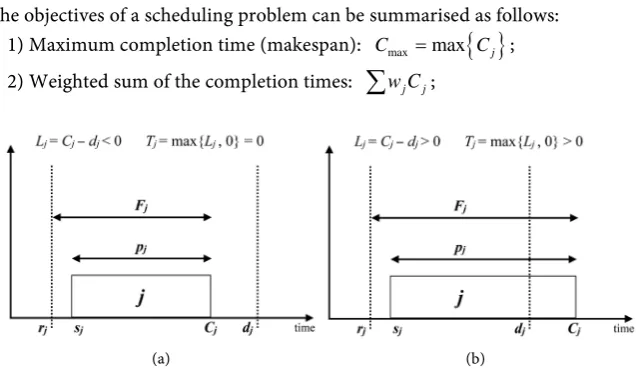
Flow time Fj=Cj−rj: Difference between the completion time and the
re-lease time; it is the turnaround time of the operation j;
Lateness Lj =Cj −dj: Difference between the completion time and the
ex-piry time; if Lj >0 the operation was completed late; if Lj<0, it was
com-pleted early;
Tardiness Tj =max
{ }
Lj, 0 : Only takes into account delays with respect to completion times;Slack (scroll) slj =dj − −rj pj: The possible sliding for the execution of the
operation.
Examples of possible operation scheduling based on the previous definitions are shown in Figure 1.
1.2. Objectives of a Scheduling Problem
The objectives of a scheduling problem can be summarised as follows: 1) Maximum completion time (makespan): Cmax =max
{ }
Cj ; 2) Weighted sum of the completion times:∑
w Cj j; [image:2.595.213.534.523.708.2](a) (b)
DOI: 10.4236/jamp.2019.711176 2581 Journal of Applied Mathematics and Physics 3) Weighted sum of flow times:
∑
w Fj j;4) Weighted sum of the delays:
∑
w Lj j;5) Maximum delay: Lmax =max
{ }
Lj ; 6) Maximum tardiness: Tmax =max{ }
Tj 7) Number of delayed operations:∑
δ( )
Lj1
8) Weighted number of delayed operations:
∑
wjδ( )
Lj 9) Weighted sum of the tardinesses:∑
w Tj jObjective (1) is oriented towards the efficient use of machines; objectives (2-4) are user-oriented; objectives (5-9) are time-oriented. The most important objectives are the makespan (Cmax), the weighted sum of the completion times
(
∑
w Cj j) and the maximum delay (Lmax). An objective is regular if its valuecan-not decrease as the processing time of any operation increases. A scheduling problem typically involves the following constraints:
• Each machine cannot process more than one operation at a time; • Each operation must be processed at most by one machine at a time; • An operation can be performed in the time interval r dj, j;
• Any technological constraints must be satisfied.
Some examples of technological constraints may be:
1) Possibility to interrupt the execution of an operation and to resume it later (preemptive scheduling);
2) Constraints of precedence between operations;
3) Need to wait for setup times between the completion of one operation and the start of another on the same machine;
4) Possibility to execute groups of operations simultaneously (batch scheduling).
1.3. Classification of Scheduling Problems
Scheduling problems can be classified on the basis of: characteristics of opera-tions; time constraints; type of information available.
Classification according to the characteristics of the operations.
According to the characteristics of the operations you can distinguish between: one-step problems (all jobs require only one operation and, therefore, you can talk about either job or task), multi-stage problems (each job is composed of several operations among which there are precedence constraints).
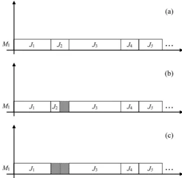
One-step problems can, in turn, be distinguished, depending on the number of machines, under (see Figure 2): single machine problems (with only one ma-chine), parallel machine problems (if there is more than one machine).
Classification according to time constraints.
Taking into account time constraints, you can distinguish among:
• Static problems: If the operations are all available at the start of the schedule
(rj =0 for each operation);
• Dynamic problems: If operations become available in time in a way known a
DOI: 10.4236/jamp.2019.711176 2582 Journal of Applied Mathematics and Physics
Figure 2. Example of single (a) and parallel (b) machine solutions for one-step scheduling problems.
• Online problems: If operations become available over time in a way not known
a priori (rj >0 not known in advance).
Classification according to the type of information available.
Considering the type of information available, scheduling problems can be:
• Deterministic, if the parameters associated with the operations (processing
times, release times, deadlines) are all deterministic;
• Stochastic, if any of the parameters associated with the operations (processing
times, release times, deadlines) are defined in random terms.
1.4. Classification of Solutions
A standard method for classifying a scheduling problem is Graham’s notation [5] where a problem is indicated by specifying three types of information: informa-tion on machines and phases; informainforma-tion related to the presence of constraints; optimization criterion.
A solution to a scheduling problem can be (see Figure 3): without delay (if it never happens that a machine, even though it can perform an operation, re-mains inactive); active (if, in order to anticipate the completion of any operation, there is a delay in the completion of other operations); inactive (if not active).
A solution without delay is also active. An active solution may be delayed. The optimal solution to a scheduling problem is an active solution but not necessari-ly without delay.
[image:4.595.280.462.517.695.2]DOI: 10.4236/jamp.2019.711176 2583 Journal of Applied Mathematics and Physics
1.5. Solution Methods
Like all optimization problems, a scheduling problem can be solved with exact or heuristic methods depending on its complexity [6] [7] [8].
A widely used construction method for solving scheduling problems is the “dispatching rules” method. It is a construction method that, in the initialisation phase, orders operations on the basis of rules or priority indexes, and then builds the solution by assigning them, in this order, to the available machines.
Priority rules are static if the value of the index does not depend on the start time of the operation, otherwise dynamic. For some problems, when the priority rule is properly chosen, the method obtains the best solution. The most com-monly used static priority rules are:
FCFS (First Come First Served): Increasing release time;
WSPT (Weighted Shortest Processing Time): Decreasing ratio wj pj or, if
1
j
w = ∀j, increasing processing time;
LPT (Longest Processing Time): Decreasing processing time; EDD (Earliest Due Date): Increasing expiry time;
MST (Minimum Slack Time): Increasing value of slack slj =dj− −rj pj
(dy-namic).
CR (Critical Ratio)
(
dj−rj)
pj : Increasing value of the ratio(
dj−rj)
pj (dynamic).The following section illustrates the scheduling problem applied to a typical CPU processing environment; then the Simulated Annealing technique is pre-sented, followed by two mathematical models formalising the scheduling prob-lem in terms of objective function and related constraints. The final sections deal with the algorithm derived from the application of SA to the CPU scheduling problem, the related computational tests and conclusions.
2. The Scheduling Problem in the Processing Environment
With reference to the management of the Central Processing Unit, it is funda-mental to have an algorithm that specifies the sequence according to which the processing service is assigned to a specific job. This algorithm is called scheduler and implements some computing methodologies which can be very time-con- suming [9] [10]. For example, it may be more expensive to run the scheduler job than the entire sequence to process.It is therefore important to indicate a “cost” function with which the weight of each possible sequence can be measured: based on this, it is necessary to find a sequence order that allows the minimisation of the cost function. It is therefore clear that scheduling issues are intimately linked to decisions about what needs to be done and how it needs to be done.
Given a problem, we will say that we can extract the sequence requests asso-ciated with this problem when the following assumptions are met:
DOI: 10.4236/jamp.2019.711176 2584 Journal of Applied Mathematics and Physics 2) The resources that can be used in the execution of the work are fully speci-fied;
3) The sequence of core tasks required to perform each of the jobs is known. The scheduling problem can be solved in several ways [11] [12]. A first way is to enumerate all the possible sequences, calculating the value of the objective function, to choose the sequence which corresponds to the lowest value of the objective function. For example if we have 10 jobs on 4 machines, we have to calculate the value of the objective function for each of the 10! possible permuta-tions. This method then becomes not available for medium and large scheduling problems.
Other classic methods that solve the problem exactly consist of algorithms for branch-and-bound [13], truncated branch-and-bound [14], dynamic program-ming [15]. In the following we will examine the solution approach known as Simulated Annealing, an approach which derives from the controlled lowering of temperature in physical systems.
3. Simulated Annealing
Simulated annealing (SA) [16] [17] [18] [19] [20] is an approach based on statis-tical mechanics concepts, and it is motivated by an analogy with the behaviour of physical systems during the cooling process. This is a heuristic method for global optimization which requires no particular assumption on the objective function (e.g. convexity).
This analogy is best illustrated in terms of the physics of single crystal forma-tion starting from a melting phase. The temperature of this “molten crystal” is then very slowly reduced until the crystal structure is formed. If cooling is car-ried out very quickly, undesirable phenomena occur as dislocations and poly-crystalline phases. In particular, very large irregularities are enclosed in the structure of the crystal and the level of potential energy incorporated is much higher than that which would exist in a perfect single crystal.
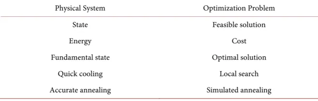
[image:6.595.209.538.619.724.2]This “quick cooling” process can be seen as similar to local optimization (Table 1). The states of the physical system correspond to the solutions of a combinatorial optimization problem; the energy of a state corresponds to the cost of a solution and the minimum energy, or fundamental state, corresponds to an optimal solution.
Table 1. The analogy between the physical system and the discrete optimization problem.
Physical System Optimization Problem
State Feasible solution
Energy Cost
Fundamental state Optimal solution
Quick cooling Local search
DOI: 10.4236/jamp.2019.711176 2585 Journal of Applied Mathematics and Physics When the temperature is, theoretically, at absolute zero Kelvin no state transi-tion can lead to a higher energy state. Therefore, as in local optimizatransi-tion, upward movements are forbidden and the consequences of this may be undesirable.
When crystals begin to form, the risk of undesirable local states is avoided by lowering the temperature very slowly, with a process called accurate annealing. In this process the temperature drops very slowly through a series of levels, each maintained long enough to allow the search for equilibrium—at that tempera-ture—for the crystal. As long as the temperature is larger than zero Kelvin, up-ward movements are always possible. By not allowing the temperature to deviate from that one compatible with the energy level of the current equilibrium, we can hope to avoid local optima until we are relatively close to the basic state.
SA is the algorithmic counterpart of this physical annealing process. Its name refers to the technique of simulation of the physical annealing process in con-junction with an annealing schedule of temperature decrease. It can be seen as an extension of the local optimization technique [21] [22] [23] [24], where the initial solution is repeatedly improved by small local perturbations until none of these perturbations improves the solution. SA randomizes this procedure in such a way as to occasionally allow upward movements, i.e. perturbations that worsen the solution, and this in an attempt to reduce the probability of blocking in a locally optimal but overall poor solution.
This technique was proposed by [25] and used in the field of statistical physics to determine the properties of metal alloys at a given temperature. The possibili-ty of solving combinatorial optimization problems have been demonstrated in-dependently by [26] and [27]. Further applications have been carried out with great success, as shown in [28] [29] [30] [31].
A simple scheme of simulated annealing is as follows: 1) Consider an initial solution S
2) Until you have a freeze
a) For w: 0= up to the number of neighbors considered i) Let S’ an unexamined neighbor of S
ii) If Cost(S’) < Cost(S) then S:=S′
else set S:=S′ with a certain probability
b) Cool the temperature 3) Return S
From what reported above it is clear that the fundamental parameters for the SA phase are:
Freezing. This consists of establishing the criteria for stopping the algorithm. Temperature. This is a value on which the probability of accepting upward movements depends. At each iteration this temperature is reduced by a constant rate called cooling.
Number of neighbors to explore. Each iteration considers a (fixed) number of sequences close to the one considered.
DOI: 10.4236/jamp.2019.711176 2586 Journal of Applied Mathematics and Physics out of locally excellent but globally poor solutions by allowing upward move-ments with a certain probability.
4. Mathematical Models
In Subection 1.1, we indicated with the term completion time (Cj) a value that
depends on the particular scheduling sequence. If a job is in position j in the se-quence, its completion time is the completion time of the job at position j−1 plus its processing time. We will denote with the term total completion time the sum of the completion times of each individual job.
The sequencing problems that we will deal with are called non preemptive: the job that is in the processing state cannot be interrupted for any reason.
For the solution of scheduling problems we describe two mathematical mod-els [32] that formalise it. The first model formulates the problem of scheduling n jobs on m machines that minimises the total completion time. We indicate with
k ij
x the variable that is equal to 1 if job j is the k-th job executed on the machine
i, 0 otherwise. We also indicated pij the processing time of job j on machine i.
The model is therefore as follows:
(
)
(
)
{ } (
)
1 1 1
1 1
1
Minimize subject to :
1 1, ,
1 1, , ; 1, ,
0,1 1, , ; , 1, ,
m n n
k ij ij
i j k
n m k ij k i n k ij j k ij p x
x j n
x k n i m
x i m j k n
= = = = = = = = ≤ = = ∈ = =
∑∑∑
∑∑
∑
where the first constraint binds the j-th job to run as k-th on the i-th machine for some i and j.
The second model concerns the scheduling of n jobs on m machines that mi-nimizes the sum of the single completion times. By specifying with
1
k
k l
ij ij ij l
C p x
=
=
∑
the completion time of job j scheduled as k-th on machine i, therelated mathematical model is therefore:
(
)
(
)
{ } (
)
1 1 1
1 1
1
Minimize subject to :
1 1, ,
1 1, , ; 1, ,
0,1 1, , ; , 1, ,
m n n
k ij
i j k
n m k ij k i n k ij j k ij C
x j n
x k n i m
x i m j k n
= = = = = = = = ≤ = = ∈ = =
∑∑∑
∑∑
∑
5. The Simulated Annealing Algorithm
DOI: 10.4236/jamp.2019.711176 2587 Journal of Applied Mathematics and Physics m machines establishing that the order of the n jobs is the same on each of the m machines.
5.1. Basic Parameters
Basic parameters for the phase of simulated annealing are:
Initialization. Choice of an initial solution. In theory the choice of an initial solution has no effect on the quality of the final solution, i.e. the solution con-verges to the overall optimum independently of the initial solution [36]. There are, however, experimentally verified exceptions to this theory, in which it has been shown that sometimes the process of convergence to the optimal solution is more rapid if one takes as the initial solution a solution obtained by means of a good heuristic [37]. However, the overall computational time for an approx-imate solution starting from a “good” initial solution is often higher than the computational time needed to obtain an approximate solution starting from any initial solution. The reason for this approach is to be found in the peculiarity of the mechanism that generates the perturbations.
Selection of a mechanism that generates small perturbations, to pass from one configuration to another one. The perturbation pattern is a crucial element to obtain good performances. The chosen perturbation scheme consists in con-sidering two randomly generated numbers and exchanging places for the jobs that in the scheduling queue occupy the positions relative to the random num-bers chosen.
5.2. Data Structure
The data structure chosen for the representation of the j-th job (with
0< ≤ −j n 1) implements the most important definitions of Subsection 1.1 as follows:
( )
, 0 1p i ∀ ≤ ≤ −i m
It is a vector that stores the job’s processing time on the i-th processor (ma-chine). These data are read from the input stream.
totp
This is the total processing time of the job, obtained by summing the processing time of the job on all processors =
( )
1
m i
p i
=
∑
.d
Job due date. This data is read from the input stream and is calculated by the generator in the following way:
(
input percentage of)
p p
d =tot + tot
c
com-DOI: 10.4236/jamp.2019.711176 2588 Journal of Applied Mathematics and Physics pletion time of the job that precedes it in the scheduling queue plus its own processing time.
late
This is the late work [12] value of the job. It is computed as follows:
• If c− ≤d 0 then late=0
• If 0< − ≤c d totp then late= −c d • If c d− >totp then late=totp
Other useful information for understanding the algorithm are: Actual order
This is the scheduling order of the jobs currently considered. The order fol-lowing the reading of the data from the input stream is assumed to be
0,1, 2,,n−1. Best order
It is the job scheduling order that obtains the minimum from the objective function. This minimum value is stored in the variable BOF (Best Objective Func-tion).
Parameters chosen for the simulated annealing phase are: Freezing criterion
A freeze occurs when the algorithm, for MAXITERATIONS times, does not perform neither a downhill nor an uphill movement.
Temperature
The initial temperature for the simulated annealing phase is set in the temper-ature parameter.
Cooling
At each iteration, the temperature is cooled by this parameter. L
Number of neighbors to visit at each iteration.
5.3. The Proposed Algorithm
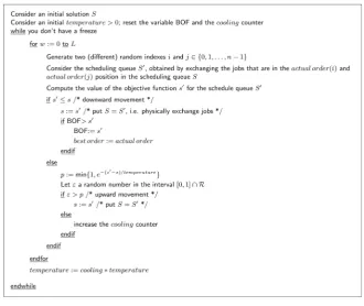
The proposed algorithm consists of two nested cycles. Basically, it chooses two integer random numbers (i and j) in the range
{
0,1,,n−1}
; then exchanges job i and job j in the scheduling queue; finally it calculates the value of the objec-tive function. If this value is lower than the value stored in BOF, the scheduling order is stored and the variable BOF is updated. Otherwise, if the value worsens the objective function, a probability is computed on the basis of which the wor-sening of the objective function is accepted.The detailed algorithm is shown in Figure 4. Its strength lies in computing the value of the objective function without having to physically exchange jobs i and j.
5.4. Application Example
DOI: 10.4236/jamp.2019.711176 2589 Journal of Applied Mathematics and Physics
[image:11.595.210.540.388.541.2]Figure 4. The proposed algorithm.
Table 2. Initial job sequence.
actual order 0 1 2 3 4 5 6
Machine 0 10 40 80 30 50 15 70
Machine 1 8 45 87 22 52 13 75
Machine 2 12 30 85 20 50 18 48
totp 30 115 252 72 152 46 193
d 33 126.5 277.2 79.2 167.2 50.6 212.3
c 30 145 397 469 621 667 860
late 0 18.5 119.8 72 152 46 193
best order 0 1 2 3 4 5 6
Table 3. Permuted job sequence.
actual order 0 1 4 3 2 5 6
Machine 0 10 40 50 30 80 15 70
Machine 1 8 45 52 22 87 13 75
Machine 2 12 30 50 20 85 18 48
totp 30 115 152 72 252 46 193
d 33 126.5 167.2 79.2 277.2 50.6 212.3
c 30 145 297 369 621 667 860
late 0 18.5 129.8 72 252 46 193
[image:11.595.209.539.570.739.2]DOI: 10.4236/jamp.2019.711176 2590 Journal of Applied Mathematics and Physics In this case we have worsened the value of the objective function (the late work values for jobs 2 and 4 increased). In fact the best order queue is unchanged, but it remains evident that the completion time values:
• for the first two positions (job 0 and job 1) remained unchanged (respectively
30 and 145, being their positions unaltered);
• for positions 2 (now job 4) and 3 (job 3, unchanged) have been decreased by
the same amount (100); this decrease is precisely equal to the difference
( )
4( )
2p p
diff =tot −tot of the initial scheme;
• for the jobs at positions 4 (now job 2), 5 (job 5, unchanged) and 6 (job 6,
un-changed) remained the same.
For late work values (see 5.2) we have instead:
• late has not changed for jobs 0 and 1 in the new scheduling queue;
• for job 4 (that occupies position 2 in the new queue) we have
0< − =c d 297 167.2− =129.8≤totp=152⇒late= − =c d 129.8;
• for job 3 we have c− =d 369 79.2− =289.8>totp =72⇒late=totp =72;
• for job 2 (at position 4 in the new scheduling queue) we have
621 277.2 343.8 p 252 p 152
c− =d − = >tot = ⇒late=tot = ;
• for jobs 5 and 6 the late values are unchanged.
In general, if we intend to exchange job i with job j (i< j):
• the values of late work will be unchanged for jobs in positions
{
0,1,,i−1}
;• the following value is computed: diff =totp
( )
j −totp( )
i ;• for job in position i, the new late work value is calculated by comparing the
quantity: diff +c i
( ) ( )
−d j with the due date value of process j;• for jobs in position
{
i+1,i+2,,j−1}
the late work value is computed by comparing the quantity: diff +c k( ) ( )
−d k with the due date value of processk, where k∈ +
{
i 1,i+2,,j−1}
;• for job in position j the new late work value is computed by comparing the
quantity: diff +c j
( ) ( )
−d i with the due date value of process i;• for jobs in position
{
j+1,j+2,,n−1}
the late work values are un-changed.We can therefore compute the value of the objective function without having to build the tables for the new schedule queue, but simply by processing infor-mation that is already available without using memory quantities.
6. Computational Tests
Before analyzing the computational tests, let us consider the (random) generator of the numbers that form the processing time values. For each job on each ma-chine a random integer number is generated in the range
[
0,100]
which represents the processing time value of the job on the processor.DOI: 10.4236/jamp.2019.711176 2591 Journal of Applied Mathematics and Physics Data to be considered common to all tests are:
• increase percentage for the due date values: 10; • number of neighbors to be explored: 10; • number of iterations per problem: 15.
With regard to the number of neighbors to be explored, the above value was chosen because from an experimental check it was noted that for a smaller number (of neighbors) you get results close to the optimal one, while for a larger number you will keep (in the cases we tested) values that often coincide with the optimal one but, being computationally severe, they negatively affect the execu-tion time of the approximaexecu-tion algorithm.
Some test cases are presented to verify the computational weight on the basis of the hypotheses made.
[image:13.595.55.545.578.727.2]Guidance for understanding computational testing.
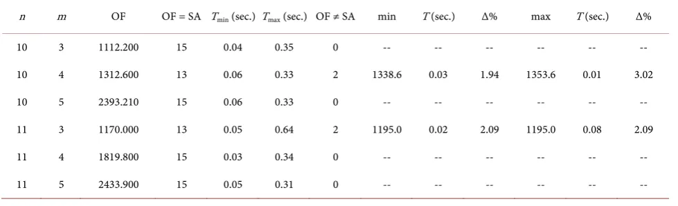
Table 4 summarises the tests performed. The indications at the top of the columns indicate:
n: number of jobs to be scheduled; m: number of machines used;
OF: optimum value of the objective function;
OF = SA: number of times that the result obtained with the approximated al-gorithm of simulated annealing coincides with the optimal one;
Tmin: minimum time (in seconds) taken by the simulated annealing algorithm
to find a result that coincided with the optimum;
Tmax: maximum time (in seconds) taken by the simulated annealing algorithm
to find a result that coincided with the optimum;
OF ≠ SA: number of times the result obtained by the approximated simulated annealing algorithm differs from the optimum one;
min: minimum value used by the simulated annealing algorithm to obtain a result that does not coincide with the optimum;
T: time (in seconds) taken by the simulated annealing algorithm to obtain a result that does not coincide with the optimum;
Δ%: average percentage difference.
Table 4. Computational tests.
n m OF OF = SA Tmin (sec.) Tmax (sec.) OF ≠ SA min T (sec.) Δ% max T (sec.) Δ%
10 3 1112.200 15 0.04 0.35 0 -- -- -- -- -- --
10 4 1312.600 13 0.06 0.33 2 1338.6 0.03 1.94 1353.6 0.01 3.02
10 5 2393.210 15 0.06 0.33 0 -- -- -- -- -- --
11 3 1170.000 13 0.05 0.64 2 1195.0 0.02 2.09 1195.0 0.08 2.09
11 4 1819.800 15 0.03 0.34 0 -- -- -- -- -- --
DOI: 10.4236/jamp.2019.711176 2592 Journal of Applied Mathematics and Physics
7. Conclusions
In this paper we present a randomised algorithm using the heuristic technique of Simulated Annealing (SA)—which proved its positive result as a single-state op-timization search algorithm for both discrete and continuous problems—for solving scheduling problems. The main goal behind our randomisation is to im-prove the solutions generated by classical job scheduling algorithms using SA to explore the search space in an efficient manner. The proposed hybrid algorithm were evaluated, and the experimental results show that it provides a perfor-mance enhancement in terms of best solutions and running time when com-pared to job scheduling and SA as stand-alone algorithms.
The followed solution method is of a non-deterministic type. It is based on the probability of obtaining an optimal solution in relation to the current situation of the objective function and the possible improvement due to a controlled move-ment in the space of the feasible solutions—linked to the concept of “tempera-ture” of the algorithm—until it reaches the freezing point, that is an optimal ac-ceptable one.
The choice made in our method prescinds from the initial solution and it ra-ther takes into account the total computing time required, since it is more im-portant to obtain an “almost” optimal feasible solution in a reasonable time rather than trying to arrive at the optimal solution in a theoretically unlimited time.
Conflicts of Interest
The authors declare no conflicts of interest regarding the publication of this pa-per.
References
[1] Kan, A.R. (2012) Machine Scheduling Problems: Classification, Complexity and Computations. Springer Science & Business Media, New York.
[2] Horn, W.A. (1974) Some Simple Scheduling Algorithms. Naval Research Logistics Quarterly, 21, 177-185. https://doi.org/10.1002/nav.3800210113
[3] Błażewicz, J. (1987) Selected Topics in Scheduling Theory. North-Holland Mathe-matics Studies, 132, 1-59. https://doi.org/10.1016/S0304-0208(08)73231-6
[4] Jain, A.S. and Meeran, S. (1998) A State-of-the-Art Review of Job-Shop Scheduling Techniques. Technical Report, Department of Applied Physics, Electronic and Me-chanical Engineering, University of Dundee, Dundee, Scotland.
[5] Mason, E.A. and Kronstadt, B. (1967) Graham’s Laws of Diffusion and Effusion. Journal of Chemical Education, 44, 740.https://doi.org/10.1021/ed044p740
[6] Abraham, A., Buyya, R. and Nath, B. (2000) Nature’s Heuristics for Scheduling Jobs on Computational Grids. The 8th IEEE International Conference on Advanced Computing and Communications (ADCOM 2000), 45-52.
[7] Kaplanoğlu, V. (2016) An Object-Oriented Approach for Multi-Objective Flexible Job-Shop Scheduling Problem. Expert Systems with Applications, 45, 71-84. https://doi.org/10.1016/j.eswa.2015.09.050
Prob-DOI: 10.4236/jamp.2019.711176 2593 Journal of Applied Mathematics and Physics lem: Conventional and New Solution Techniques. European Journal of Operational Research, 93, 1-33. https://doi.org/10.1016/0377-2217(95)00362-2
[9] Çaliş, B. and Bulkan, S. (2015) A Research Survey: Review of AI Solution Strategies of Job Shop Scheduling Problem. Journal of Intelligent Manufacturing, 26, 961-973. https://doi.org/10.1007/s10845-013-0837-8
[10] Jamali, S., Alizadeh, F. and Sadeqi, S. (2016) Task Scheduling in Cloud Computing Using Particle Swarm Optimization. The Book of Extended Abstracts, 192.
[11] Gonzalez, T.F. (2007) Handbook of Approximation Algorithms and Metaheuristics. Chapman and Hall/CRC, New York.
[12] Potts, C.N. and Van Wassenhove, L.N. (1992) Approximation Algorithms for Scheduling a Single Machine to Minimize Total Late Work. Operations Research Letters, 11, 261-266. https://doi.org/10.1016/0167-6377(92)90001-J
[13] Morrison, D.R., Jacobson, S.H., Sauppe, J.J. and Sewell, E.C. (2016) Branch-and- Bound Algorithms: A Survey of Recent Advances in Searching, Branching, and Pruning. DiscreteOptimization, 19, 79-102.
https://doi.org/10.1016/j.disopt.2016.01.005
[14] Sels, V., Coelho, J., Dias, A.M. and Vanhoucke, M. (2015) Hybrid Tabu Search and a Truncated Branch-and-Bound for the Unrelated Parallel Machine Scheduling Problem. Computers & Operations Research, 53, 107-117.
https://doi.org/10.1016/j.cor.2014.08.002
[15] Bellman, R.E. and Dreyfus, S.E. (2015) Applied Dynamic Programming. Volume 2050, Princeton University Press, Princeton, NJ.
[16] Krishnaraj, J., Pugazhendhi, S., Rajendran, C. and Thiagarajan, S. (2019) Simulated Annealing Algorithms to Minimise the Completion Time Variance of Jobs in Per-mutation Flowshops. International Journal of Industrial and Systems Engineering, 31, 425-451.https://doi.org/10.1504/IJISE.2019.099188
[17] Ogbu, F.A. and Smith, D.K. (1990) The Application of the Simulated Annealing Algorithm to the Solution of the n/m/Cmax Flowshop Problem. Computers & Op-erations Research, 17, 243-253.https://doi.org/10.1016/0305-0548(90)90001-N [18] Chakraborty, S. and Bhowmik, S. (2015) An Efficient Approach to Job Shop
Sche-duling Problem Using Simulated Annealing. International Journal of Hybrid In-formation Technology, 8, 273-284.https://doi.org/10.14257/ijhit.2015.8.11.23 [19] Cruz-Chávez, M.A., Martínez-Rangel, M.G. and Cruz-Rosales, M.H. (2017)
Accele-rated Simulated Annealing Algorithm Applied to the Flexible Job Shop Scheduling Problem. International Transactions in Operational Research, 24, 1119-1137. https://doi.org/10.1111/itor.12195
[20] Sel, C. and Hamzadayi, A. (2015) A Simulated Annealing Approach Based Simula-tion-Optimization to the Dynamic Job-Shop Scheduling Problem. Pamukkale Uni-versity Journal of Engineering Sciences, 24,665-674.
[21] Akram, K., Kamal, K. and Zeb, A. (2016) Fast Simulated Annealing Hybridized with Quenching for Solving Job Shop Scheduling Problem. Applied Soft Computing, 49, 510-523.https://doi.org/10.1016/j.asoc.2016.08.037
[22] Bissoli, D.C., Altoe, W.A.S., Mauri, G.R. and Amaral, A.R.S. (2018) A Simulated Annealing Metaheuristic for the Bi-Objective Flexible Job Shop Scheduling Prob-lem. 2018 International Conference on Research in Intelligent and Computing in Engineering, San Salvador, El Salvador,22-24 August 2018, 1-6.
https://doi.org/10.1109/RICE.2018.8627907
DOI: 10.4236/jamp.2019.711176 2594 Journal of Applied Mathematics and Physics Problem under Fuzzy Processing Time Using the Simulated Annealing Method. Journal of Progressive Research in Mathematics, 14, 2308-2317.
[24] Shivasankaran, N., Kumar, P.S. and Raja, K.V. (2015) Hybrid Sorting Immune Si-mulated Annealing Algorithm for Flexible Job Shop Scheduling. International Journal of Computational Intelligence Systems, 8, 455-466.
https://doi.org/10.1080/18756891.2015.1017383
[25] Metropolis, N., Rosenbluth, A.W., Rosenbluth, M.N., Teller, A.H. and Teller, E. (1953) Equation of State Calculations by Fast Computing Machines. The Journal of Chemical Physics, 21, 1087-1092.https://doi.org/10.1063/1.1699114
[26] Kirkpatrick, S., Gelatt, C.D. and Vecchi, M.P. (1983) Optimization by Simulated Annealing. Science, 220, 671-680.https://doi.org/10.1126/science.220.4598.671 [27] Černy, V. (1985) Thermodynamical Approach to the Traveling Salesman Problem:
An Efficient Simulation Algorithm. Journal of Optimization Theory and Applica-tions, 45, 41-51.https://doi.org/10.1007/BF00940812
[28] Aarts, E.H.L. and Van Laarhoven, P.J.M. (1985) Statistical Cooling: A General Ap-proach to Combinatorial Optimization Problems. Philips Journal of Research, 40, 193-226.
[29] Heynderickx, I., De Raedt, H. and Schoemaker, D. (1986) Simulated Anneal Me-thod for the Determination of Spin Hamiltonian Parameters from ESR Data. Jour-nal of Magnetic Resonance, 70, 134-139.
https://doi.org/10.1016/0022-2364(86)90367-7
[30] Lundy, M. (2015) Applications of the Annealing Algorithm to Combinatorial Prob-lems in Statistics. Biometrika, 72, 191-198.
[31] Vecchi, M.P. and Kirkpatrick, S. (1983) Global Wiring by Simulated Annealing. IEEE Transactions on Computer-Aided Design of Integrated Circuits and Systems, 2, 215-222.https://doi.org/10.1109/TCAD.1983.1270039
[32] Błażewicz, J., Dror, M. and Weglarz, J. (1991) Mathematical Programming Formu-lations for Machine Scheduling: A Survey. European Journal of Operational Re-search, 51, 283-300.https://doi.org/10.1016/0377-2217(91)90304-E
[33] Kolonko, M. (1999) Some New Results on Simulated Annealing Applied to the Job Shop Scheduling Problem. European Journal of Operational Research, 113, 123-136. https://doi.org/10.1016/S0377-2217(97)00420-7
[34] Osman, I.H. and Potts, C.N. (1989) Simulated Annealing for Permutation Flow-Shop Scheduling. Omega, 17, 551-557.
https://doi.org/10.1016/0305-0483(89)90059-5
[35] Van Laarhoven, P.J.M., Aarts, E.H.L. and Lenstra, J.K. (1992) Job Shop Scheduling by Simulated Annealing. Operations Research, 40, 113-125.
https://doi.org/10.1287/opre.40.1.113
[36] Lundy, M. and Mees, A. (1986) Convergence of an Annealing Algorithm. Mathe-maticalProgramming, 34, 111-124.https://doi.org/10.1007/BF01582166